Green Sunfish - USGS National Wetlands Research Center

Biological Services Program 

and 

Division of Ecological Services 

FW5/085-82/1 0.15 

JULY 1982 

70e 

bilfoyet+e 

HABITAT SUITABILITY INDEX MODELS: 

GREEN SU NFISH 

Fish and Wildlife Service 

u.s. Department of the Interior

The Biological Services Program was establfshed within the U.S. Fish 

and Wildlife Service to suppl,y scientific information and methodologies on 

ke,y envi ronmental issues thJt impact fish and wl1dlf fe resources and thei r 

supporting ecos,ystems. The mission of the program is as follows·: 

• To strengthen the Fish and Wildlife Service in its role as 

a primar,y source of information on national fish and wildlife 

resources, particularl,y in respect to environmental 

impact assessment. 

• To gath.r, antl,yze, and present information that will.aid 

decisiol'lllllkers in the identification and resolution of 

problems associated with major changes in land and water 

use. 

• To provide better ecological information and evaluation 

for Department of the Interior development prog~ams. such 

as those relating to energy development. 

Information developed by the Biological Services Program is intended 

for use in the planning and decisionmakingprocess to prevent or minimize 

tha impact of development on fish and wl1dlife. Researc:hactiv1ties and 

technical assistance services are based on an analysis of the issues, a 

determination of the decisionmakers involved and their information needs, 

and an evaluation of the state of the art to identify information gaps 

and to determine priorities. This is a strategy that will e"sure that 

the products produced and disseminated are timely and useful. 

') 

Projec;ts have been i"itiated in the following areas: coal extraction 

and conversion; power plants; geothermal, mineral andoH shale develop~ 

ment; water resource analysis. including stream alterations and western 

water allocation; coastal ecosystems and Outer Continental Shelf development; 

and systems inventory, including National Wetland Inventory, 

habitat classification and analysis, and information transfer. 

The Biological Services Program consists of the Office of Biological 

Services in Washington, D.C., which is ruponsible for overall planni"g and 

management; National TellllS, which provide the Program's central scientific; 

and technical expertise and arrange for contracting biolo!!ical services 

stUdies with states, universities, consulting firms, and others; Regional 

Staffs, who provide a link to problems at the operating level;and staffs at 

certain Fish and Wildlife Service research facilities, who conduct tn-house 

research studies. 

This model is designed to be used by the Division of Ecological Services 

in conjunction with the Habitat Evaluation Procedures.

FWS/OBS-82/10.15 

July 1982 

HABITAT SUITABILITY INDEX MODELS: GREEN SUNFISH 

by 

Robert J. Stuber 

Habitat Evaluation Procedures Group 

Western Energy and Land Use Team 

U.S. Fish and Wildlife Service 

Drake Creekside Building One 

2625 Redwing Road 

Fort Collins, CO 80526 

Glen Gebhart 

and 

O. Eugene Maughan 

Oklahoma Cooperative Fishery Research Unit 

Oklahoma State University 

Stillwater, OK 74074 


Office of Biological Services 


U.S. Department of the Interior 

Washington, DC 20240

This report should be cited as: 

Stuber, R. J., G. Gebhart, and O. E. Maughan. 1982. Habitat suitability index 

models: Green sunfish. U.S. Dept. Int. Fish Wildl. Servo 

FWS/OBS-82/10.15. 28 pp.

PREFACE 

The habitat use information and Habitat Suitability Index (HSI) models 

presented in this document are an aid for impact assessment and habitat management 

activities. Literature conce rnl nq a species' habitat requirements and 

preferences is reviewed and then synthesized into HSI models, which are scaled 

to produce an index between 0 (unsuitable habitat) and 1 (optimal habitat). 

Assumptions used to transform habitat use information into these mathematical 

models are noted, and guidelines for model application are described. Any 

models found in the literature which can also be used to calculate an HSI are 

cited, and simplified HSI models, based on what the authors believe to be the 

most important habitat characteristics for this species, are presented. 

Use of the models presented in this publication for impact assessment 

requires the setting of clear study objectives and may require modification of 

the models to meet those objectives. Methods for reducing model complexity 

and recommended measurement techniques for model variables are presented in 

Terrell et al. (in pr ep .'}." A discussion of HSI model building techniques, 

including the component approach, is presented in U.S. Fish and Wildlife 

Service (1981).2 

The HSI models presented herein are complex hypotheses of species-habitat 

relationships, not statements of proven cause and effect relationships. 

Results of mode,--performance tests, when available, are referenced; however, 

models that have demonstrated reliability in specific situations may prove 

unreliable in others. For this reason, the FWS encourages model users to send 

comments and suggestions that might help us increase the utility and effectiveness 

of this habitat-based approach to fish and wildlife planning. Please 

send comments to: 

Habitat Evaluation Procedures 




Ft. Collins, CO 80526 

ITerrell, J. W., T. E. McMahon, P. D. Inskip, R. F. Raleigh, and 

K. W. Williamson (in press). Habitat Suitability Index models: 

Appendix A. Guidelines for riverine and lacustrine applications of fish 

HSI models with the Habitat Evaluation Procedures. U.S. Fish and Wildl. 

Servo FWS/OBS 82/10.A. 

2U.S. Fish and Wildlife Service. 1981. Standards for the development of 

Habitat Suitability Index models. 103 ESM. U.S. Fish and Wildl. Servo 

Div. Ecol. Servo n.p.

CONTENTS 

PREFACE . . . . . . . . . . . . . . . . . . . . . . . . . . . . . . . . . . . . . . . . . . . . . . . . . . . . . . . . . . . . iii 

ACKNOWLEDGMENTS 

vi 

HABITAT USE INFORMATION 

Genera1 1 

Age, Growth, and Food 1 

Reproduct ion 1 

Specific Habitat Requirements.................................... 2 

HABITAT SUITABILITY INDEX (HSI) MODELS................................ 3 

Model Applicability. 3 

Mode 1 Descri pt ion - Ri veri ne 4 

~1odel Description - Lacustrine 6 

Suitability Index (SI) Graphs for 

Model Variables................................................ 6 

Ri veri ne Model................................................... 14 

Lacustrine Model 15 

Interpreting Model Outputs 23 

ADDITIONAL HABITAT SUITABILITY INDEX MODELS........................... 23 

Model 1 23 

Model 2 23 

Model 3 24 

REFERENCES 24

ACKNOWLEDGMENTS 

We would like to thank John Magnuson, (University of Wisconsin, Madison), 

and Richard Applegate (South Dakota Cooperative Fishery Research Unit) for 

reviewing the manuscript. Their review contributions are gratefully 

acknowledged, but the authors accept full responsibility for the contents of 

the document. Word processing was provided by Dora Ibarra and Carolyn Gulzow. 

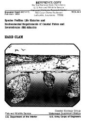
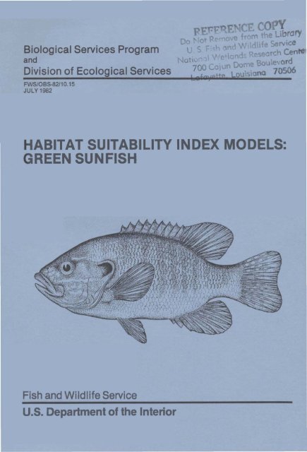
The cover of this document was illustrated by Jennifer Shoemaker.

GREEN SUNFISH (Lepomis cyanellus) 

HABITAT USE INFORMATION 

General 

The green sunfish (Lepomis cyanellus) is native from the Great Lakes 

region south to Mexico (Eddy 1957) and has been introduced both east of the 

Appalachian Mountains (Raney 1965) and west of the Rocky Mountains (Wright 

1951). The species is established in nearly every suitable habitat in the 

Western United States (McKechnie and Tharratt 1966) and is nearly ubiquitous 

within its native range (Trautman 1957; Cross 1967). Green sunfish hybridize 

with longear (1:. megalotis), orangespotted (1:. humilis), and redbreast (1. 

auritus) sunfishes, bluegill (1:. macrochirus), and pumpkinseed (1:. gibbosus) 

(Scott and Crossman 1973). 

Age, Growth, and Food 

The maximum age, length, and weight of green sunfish is about 10 years, 

276 mm, and 408 g, respectively (Carlander 1977). Age at maturity ranges from 

1 to 3 years, depending on geographic locale (Hubbs and Cooper 1935; Sprugel 

1955; Durham 1957). Males and females mature at minimum lengths of 45 (Sprugel 

1955) and 66 mm (Cross 1951), respectively. 

Adult green sunfish feed principally on insects, crayfish (Mullan and 

Applegate 1970; Etnier 1971; Applegate et a1. 1976), and fish (Biggins and 

Ziebell 1967; Mullan and Applegate 1968, 1970). Terrestrial and aquatic 

insects appear to be the most important food items (Cross 1951; Maupin et al. 

1954; McDonald and Dotson 1960). Fry initially eat zooplankton (Siewert 1973) 

and subsequently eat aquatic insects, fish eggs, and entomostraca as they grow 

larger (Applegate et al. 1976). The juvenile diet is similar to that of the 

adult (Mullan and Applegate 1968, 1970). Growth is usually faster in downstream 

river areas, where population densities are lower, than in upstream 

areas (Finnell 1955; Hoffman 1955; Jenkins and Finnell 1957; Purkett 1958). 

Reproduction 

Spawning has been noted at temperatures between 19 and 31° C (Hunter 

1963), with initial spawning usually occurring at 20 to 22° C (Swingle 1952; 

Lawrence 1957; Pflieger 1963). The male clears a nest area of about 30 cm in 

diameter (Carson 1968) and guards the nest (Hankinson 1919). Green sunfish 

nest at a depth of 4 to 35 cm (Hunter 1963; Carson 1968) on a fi rm substrate 

(Childers 1967) of gravel or sand (Hankinson 1919; Hunter 1963) near rocks, 

logs, and vegetation (Hunter 1963). 

1

Specific Habitat Requirements 

Green sunfish typically inhabit pool areas of streams (Brown 1960; 

Minckley 1963; Harlan and Speaker 1969), and optimal riverine habitat consists 

of at least 50~~ pool area. Species abundance is positively correlated with 

percent vegetative cover (Moyle and Nichols 1973). Forshage and Carter (1974) 

attributed reductions in game fish populations, which included green sunfish, 

to reductions in sheltered areas consisting of logs, brush, and gravel. More 

than 80~6 cover is assumed to be suboptimal, because it provides too much 

protection for green sunfish prey. Green sunfish have been found at a wide 

range of gradients, varying from 0.2 to 5.7 m/km (Cross 1954; Funk 1975a); 

however, they are most abundant at lower (s 2 m/km) gradients (Trautman 1957; 

Funk 1975b). They prefer small to medium-sized « 30 m width) streams 

(Trautman 1957; Cross 1967; Moyle and Nichols 1973). 

Green sunfish also thrive in lacustrine environments. Optimal habitat 

consists of fertile lakes, ponds, and reservoirs with extensive (~20% of 

lacustrine surface area) littoral areas (Scott and Crossman 1973). Optimal 

cover within littoral areas is similar to riverine criteria. Jenkins (1976) 

reported a significant positive correlation between TDS levels of 100 to 

350 ppm and sportfish (which included sunfishes) standing crop. 

Water quality criteria for green sunfish in both riverine and lacustrine 

environments are outlined as follows. High species abundance is positively 

correlated with moderate (25-100 JTU) turbidities (Trautman 1957; Cross 1967; 

Moyle and Nichols 1973), although the species occurs in both clear and turbid 

water (Jenkins and Finnell 1957). Dissolved oxygen (D.O.) requirements are 

presumably similar to those of the bluegill sunfish. Thus, optimal D.O. 

levels are> 5 mg/l (Petit 1973), and lethal levels are s 1.5 mg/l (Moore 

1942). Using Stroud's (1967) criteria for freshwater fish, optimal pH range 

is from 6.5 to 8.5. Assuming green sunfish exhibit similar responses to pH 

levels as do bluegill, mortality may occur at pH levels s 4.0 or ~ 10.35 

(Trama 1954; Calabrese 1969; Ultsch 1978). If green sunfish have salinity 

tolerances similar to those of bluegill, optimal salinities are < 3.6 ppt 

(Tebo and McCoy 1964), and green sunfish will not tolerate salinities> 5.6 ppt 

(Kilby 1955). 

Adult. The temperature preference for adult green sunfish is 28.2° C 

and, when possible, they avoid temperatures above 31° C or below 26° C 

(Bei t i nger et a l . 1975). Green sunfi sh have been found in the fi e 1d at temperatures 

as high as 36° C (Sigler and Miller 1963; Proffitt and Benda 1971). 

Growth and food conversion efficiency increased as temperature increased from 

13.2 to 28° C (Jude 1973). 

Adults are found in low current velocity areas (Gerking 1945; Brown 1960; 

Minckley 1963; Summerfelt 1967; Harlan and Speaker 1969; Moyle and Nichols 

1973). Based on catch data, preferred current velocities are ~ 10 cm/sec, but 

adults will tolerate velocities up to 25 em/sec (Kallemyn and Novotny 1977; 

Hardin and Bovee 1978). 

2

Embryo. Optimal temperature for spawning and subsequent development 

ranges from 20 to 27° C (Childers 1967). Spawning will not occur below 19° C 

or above 31° C (Hunter 1963). Optimal spawning substrate corresponds to a 

predominance (~ 50%) of sand and gravel (Hankinson 1919; Hunter 1963; Childers 

1967). Green sunfish spawn at depths of 4 to 35 em (Hunter 1963; Carson 

1968); consequently, reservoir drawdown should not exceed 1 m during spawning 

to ensure optimal embryo development and survival. Probability of use curves 

developed by Hardin and Bovee (1978) illustrate that optimal current velocity 

is ~ 10 em/sec, and embryos probably will not tolerate velocities> 15 em/sec. 

Fry. Optimal temperatures for fry range from 18 to 26° C (Siewert 1973; 

Couta~1977; Hardin and Bovee 1978). The range of tolerance for bluegill fry 

is 10 to 36° C (Banner and Van Arman 1972), and it is assumed that green 

sunfish fry tolerances are similar. Optimal current velocities are ~ 5 em/sec, 

and fry avoid areas with velocities exceeding 8 em/sec (Kallemyn and Novotny 

1977; Hardin and Bovee 1978). 

Juvenile. Specific requirements for juveniles are assumed to be the same 

as those for the adult life stage. 

HABITAT SUITABILITY INDEX (HSI) MODELS 

Model 

Applicability 

Geographic area. The models are applicable throughout the native and 

introduced range of the green sunfi sh in North Ameri ca. The standard of 

comparison for each individual variable suitability index is the optimal value 

of the variable that occurs anywhere within this region. Therefore, the 

models will never provide an HSI of 1.0 when applied to bodies of water in the 

North where temperature related variables do not reach the optimal values that 

occur in the South. 

Season. The models provide a rating for a body of water based on its 

ability to support a reproducing population of green sunfish during all seasons 

of the year. 

Cover types. The models are applicable in riverine, lacustrine, 

palustrine, and estuarine habitats, as described by Cowardin et al. (1979). 

Minimum habitat area. Minimum habitat area is defined as the minimum 

area of contiguous suitable habitat that is required for a species to live and 

reproduce. No attempt has been made to establish a minimum habitat size for 

green sunfi sh. 

Verification level. The acceptable output of these green sunfish models 

is to produce an index between 0 and 1 which the authors believe has a positive 

relationship to carrying capacity. Acceptance was based on model predictions 

using sample data sets. These sample data sets and their relationship 

to model verification are discussed in greater detail following presentation 

of the mode 1. 

3

Model Description - Riverine 

Ri veri ne green sunfi sh habi tat is assumed to be composed of food and 

cover, water quality, and reproduction components. Variables that have been 

shown to affect growth, survival, distribution, or abundance were placed in 

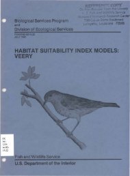
the appropriate life requisite component (Fig. 1). Variables that did not 

appear to be related to a specific life requisite component were placed in the 

"other" component. 

Information describing cause and effect relationships of variables and 

components in determining habitat suitability was lacking. We assumed that 

high values for one life requisite or variable would compensate for lower 

values of another life requisite, except when values for a variable approached 

levels that had clearly demonstrated negative impacts on growth or survival. 

Food and cover component. Percent bottom cover (VI) is assumed to be 

important because bottom cover provides habitat for aquatic insects, crayfish, 

and small fish which are the predominant food items of green sunfish. Bottom 

cover also provides resting areas with low current velocities and protection 

from predation. Species abundance has been positively correlated with percent 

cover. Percent pools (V 2 ) is included to quantify the amount of habitat 

actually used by the speci es. Food and cover have been aggregated into one 

component because the fish have a tendency to feed near cover. 

Water guality component. The water quality component is limited to 

dissolved oxygen (V4), turbidity (V s ), pH (V G ) , temperature (V 7 , V s ), and 

salinity (V 18 ) measurements. The salinity measurement is optional. These 

parameters have been shown to affect growth or survival. Variables related to 

temperature and oxygen were assumed to be limiting when they reach near-lethal 

levels. Toxic substances were not considered in this model. 

Reproduction component. Temperature for spawning (V g ) describes water 

quality conditions that affect embryonic development. Substrate (V lO ) is 

important in determining spawning success. Current velocity (V 12 ) within 

pools during spawning is important because developing eggs will not survive in 

areas with velocities> 15 cm/sec. 

Other component. The va ri ab 1es whi ch are in the other component also 

describe habitat suitability for the green sunfish, but are not specifically 

related to life requisite components already presented. Stream gradient (V 3 ) 

is included because green sunfish are most abundant in streams with lower 

gradients ($ 2 m/km). Current velocity (VII' V 1 3 ) is important because green 

sunfish prefer low velocity areas. Stream width (V I 4) further describes 

preferred habitat because small to medium-sized streams « 30 m width) are 

most suitable. 

4

Habitat Variables 

Life Requisites 

% 0 f bottom cou~ve:r~e~d~(~V~l~)-==========:::==- 

_ 

Food-cover (CF-C) 

Dissolved oxygen (V 4 ) 

Turbi d it'JY~(V~5~)~=========;;;;~~~ 

- Water quality (C WQ) 

Temperature (V 7 

----- 

, Va) 

Salinity (V 18 ) 

HSI 

Temperature (V 9 ) 

Substrate (V,,)~ Reproduction (C R) 

Current velocity (V 1 Z ) 

Stream gradient (V 3 ) 

Current velocity(V~Other (COT) 

Stream width (V 1 4 ) 

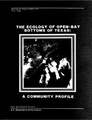
Figure 1, Tree diagram illustrating relationship of habitat variables 

and life requisites in the riverine model for green sunfish. The 

dashed line indicates an optional variable. 

5

Model Description - Lacustrine 

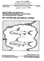
Lacustrine habitat suitability was assumed to be determined by the same 

life requisite components as riverine habitat suitability (Fig. 2). Little 

information was available to determine how variables combine to determine 

habitat suitability. We assumed that compensation for one life requisite 

value by another life requisite value occurs except when values for a variable 

approach levels that have clearly demonstrated negative impacts on growth or 

survival. 

Food component. Average TDS (VIS) is included because the TDS is a 

measure of lacustrine productivity. There is a positive correlation between 

sunfish standing crops and TDS levels, presumably due to the greater amount of 

food organisms produced at higher TDS levels. 

Cover component. Percent bottom cover (VI) is included because species 

abundance is positively correlated with percent cover. Bottom cover provides 

resting areas and protection from predation. Percent littoral area (V 1 6 ) 

quantifies the amount of cover habitat. 

Water qual ity component. Same explanation as presented in the riverine 

model description. 

Reproduction component. Temperature for spawning 

quality conditions that affect embryonic development. 

important in determining spawning success. Reservoir 

included because optimal embryo development and survival 

stable water levels during spawning. 

(V g ) describes water 

Substrate (V lO ) is 

drawdown (V 17 ) is 

a re dependent on 

Suitability Index (SI) Graphs for Model 

Variables 

This section contains suitability index graphs for the 18 variables 

described above and equations that quantify assumptions for combining selected 

variable indices into a species HSI with the component approach. The IIR II 

pertains to riverine habitat variables, and the IIL II refers to lacustrine 

habitat variables. 

6

Habitat Variables 

Life Requisites 

Average TDS (V 1 S ) ---------- Food (C F) 

% of stream bottom covered (V 1 ) 

Cover (CC) 

~ littoral area (V 1 6 ) 

Dissolved oxygen 

Turbidity (V s ) 

pH (V 6 ) -------------~ Water Qual ity (C WQ) 

-----~ HSI 

---- 

Temperature _--- 

Sa1in ity (V 18) ...... - 

Temperature (V g )~ 

Substrate (V 1 0 ) ------------------------------------~ Reproduction (C R) 

Reservoir drawdown (V 1 7 ) 

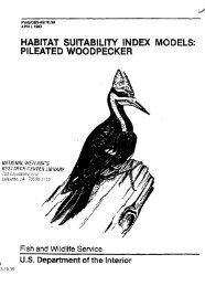
Figure 2. Tree diagram illustrating relationship of habitat variables 

and life requisites in the lacustrine model for green sunfish. The 

dashed line indicates an optional variable. 

7

Habitat 

Variable 

R,L 

Percent of the bottom 

of pools or littoral 

areas covered with 

vegetation, rocks, or 

debris during summer. 

R Percent pool area 

during average summer 

flow. 

1.0 

>< 

-& 0.8 

t:: 

~ 0.6 

'r- 

:0 0.4 

ttl 

+-> 

...... 

~ 0.2 

0.0 

0 25 50 

% 

75 100 

8

R 

Stream gradient within 

representative reach. 

1.0 

~ 0.8 

-0 

t:: 

........ 

>, 0.6 

+J 

...... 

:; 0.4 

~ 

+J 

...... 

~ 0.2 

0.0 

0 2 4 6 

m/km 

8 10 

R,L 

Minimum dissolved oxygen 

levels during summer. 

A) Usually> 5 mg/l 

B) Usually 4-5 mgjl 

C) Usually 2-4 mg/l 

D) Frequently ~ 2 mg/l 

Note: 

Lacustrine D.O. 

levels refer to 

littoral areas. 

1.0 

~ 0.8 

-0 

t:: 

........ 

>, 0.6 

+J 

.,- 

:;=0.4 

.o 

~ 

+J 

.; 0.2 

(/) 

0.0 

- ~ 

A B C D 

R,L V s Maximum monthly average 1.0 

turbidity within pools 

or littoral areas during x 0.8 

the summer. 

OJ 

-0 

t:: 

........ 

>, 0.6 

+J 

...... 

...... 0.4 

..0 

~ 

+J 

:::i 0.2 

(/) 

9 

0.0 

0 50 100 150 200 

JTU

R,L pH range during summer 

growing season. 

A) 6.5-8.5 

B) 5.0-6.5 or 8.5-9.0 

C) 4.0-5.0 or 9.0-10.0 

D) < 4.0 or > 10.0 

1.0 

x 0.8 

Q) 

"0 

t:: 

...... 0.6 

>, 

+' 

'r- 

0.4 

..c to 

+' 

0.2 'r- 

~ 

V) 

0.0 

A B C o 

~ 

~ 

R,L V 7 Maximum midsummer 1.0 

temperature within 

pools or littoral x 

Q) 

areas (Adult, Juvenile). 

0.8 

"0 

...... 

t:: 

>, 0.6 

+' 

'r- 

r- 

0.4 

'r- 

..c to 

+' 

'r- 

~ 

V) 

0.2 

R,L VB Maximum midsummer 1.0 

temperature within 

pools or littoral 

areas (Fry). 

x 

Q) 

"0 

0.8 

...... 

t:: 

>, 0.6 

+' 

'r- 0.4 

..c 

to 

+' 

~ 0.2 

V) 

0.0 

10 20 30 40 

DC 

0.0 

10 20 30 40 

DC 

10

R,L 

Maximum temperature 

within pools or 

littoral areas during 

spawning (June-July) 

(Embryo) . 

1.0 

x 

OJ 

"0 0.8 

C 

...... 

~ 0.6 

...... 

~ 

...... 

..0 

ttl 

+> 

...... 

::l 

(/) 

0.4 

0.2 

0.0 

10 20 30 40 

R,L V10 Substrate composition 

within pools or littoral 

areas for spawning 

(Embryo) . 

A) Boulder (> 20 cm) 

and bedrock predominate 

(~ 50%). 

B) Cobble (5-20 cm) 

predominates. 

C) Silt and sand 

(:5 0.2 cm) 

predominate. 

D) Pebbles and gravel 

(0.2-5.0 cm) 

predominate. 

1.0 

x 

OJ 

0.8 "0 

c 

...... 

~ 0.6 

..... 

..0 

ttl 0.4 

+> 

..... 

::l 

(/) 

0.2 

0.0 

A 

B 

C 

D 

~ 

~ 

R V ll Average current velocity 

within pools during 

average summer flow 

(Adult, Juvenile). 

1.0 

x 0.8 

OJ 

"0 

C 

...... 0.6 

>, 

+> 

...... 

~ 

...... 0.4 

..0 

ttl 

+> 

...... 

::l 0.2 

(/) 

0.0 

0 10 20 30 40 

em/sec 

11

R V 12 Average current velocity 1.0 

withi n pools during 

spawning (June-July) x OJ 0.8 

(Embryo) . -0 

c: 

....... 

>, 0.6 

~ 

...Cl 

0.4 

ro 

~ 

:::s 0.2 

Vl 

0.0 

0 5 10 15 20 

em/sec 

R V 13 Average current velocity 1.0 

within average pools during 

summer flow x OJ 0.8 

(Fry). 

-0 

c: 

....... 

>, 0.6 

~ 

...Cl 0.4 

ro 

~ 

:::s 0.2 

Vl 

0.0 

0 2 4 6 8 10 

em/sec 

R V14 Average stream width 1.0 

withi n representative 

reach. 

x 0.8 

OJ 

-0 

c: 

....... 

0.6 

>, 

~ 

0.4 

...Cl 

ro 

~ 

:::s 

0.2 

Vl 

0.0 

0 10 20 30 40 

m 

12

1.0 

L V15 Average TD5 level during 

growing season when the 

carbonate-bicarbonate >< 0.8 

Q) 

"'0 

ionic concentration> 

...... s::: 

sulfate-chloride ionic 0.6 

>, 

concentration. If the 

+-l 

sulfate-chloride ionic 

0.4 

concentration> than .0 

co 

the carbonate- 

+-l 

bicarbonate ionic :::J 

0.2 

tf) 

concentration, the 51 

rating should be 0.0 

lowered by 0.2. 51 0 200 400 600 800 

cannot be < O. 

ppm 

L V l6 Percent 1i ttora1 area 1.0 

at summer water levels. 

x 

Q) 

"'0 

0.8 

...... s::: 

c-, 0.6 

+-l 

.0 0.4 

co 

+-l 

:::J 

tf) 

0.2 

0.0 

0 25 50 75 100 

% 

L V17 Reservoir drawdown during 1.0 

spawning (Embryo). 

>< 0.8 

Q) 

"'0 s::: 

...... 

>, 

0.6 

+-l 

.0 

m+-l 

0.4 

:::J 

0.2 

tf) 

0.0 

0.0 0.5 1.0 

m 

13

Maximum monthly average 

salinity during growing 

1.0 

season (Optional). 

Q) 0.8 

"'0 

Note: V 18 can be omitted 

s:: 

...... 

if sal inity is not 

~ 0.6 

considered to be a ...... 

potential problem ...... 0.4 

within the study 

..c 

to 

+-l 

area. ..... 

::::l 

Vl 

0.2 

0.0 

0 2 4 6 8 

ppt 

Riverine Model 

These equations utilize the life requisite approach and consist of four 

components: food and cover; water quality; reproduction; and other. 

Food and Cover (C F/ C)' 

Water Quality (C WQ)' 

2V 4 + Vs + Vs + V 7 + Vs + ViS 

7 

If V 4 , V 7 , or Vs ~ 0.4, C WQ 

equals the lowest of the following: 

V 4 ; V 7 ; Vs; or the above equation. 

14

Note: If VIS (optional salinity variable) is omitted, 

V7 

+ VS 

2V 4 + V s + V 6 + 2( 2 ) 

6 

Reproduction (C R). 

2.5 

HSI 

determination. 

If CWQ is ~ 0.4, the HSI equals the lowest of the following: 

CWQ 

or the above equation. 

Lacustrine Model 

These equations utilize the life requisite approach and consist of four 

components: food; cover; water quality; and reproduction. 

15

Water Quality (C WQ)' 

V 7 + Va 

2V 4 + Vs + Vs + 2( 2 ) + V1a 

7 

If V 4 , V 7 , or Va ~ 0.4, C WQ 

equals the lowest of the following: 

V 4 ; V 7 ; Va; or the above equation. 

Note: 

If V1a (optional salinity variable) is omitted, 

2V 4 

V 7 

+ Vs + Vs + 2( 

+ Va 

2 ) 

6 

Reproduction (C R). 

Note: V 1 7 should be omitted if the lacustrine environment 

is a natural lake or pond. Thus, 

HSI determination. 

HSI (C C C CR) 1/ 4 

= F x C x WQ x 

If C WQ 

or C R 

~ 0.4, the HSI equals the lowest of the following: C WQ 

; 

C R; 

or the above equation. 

Sources of data and assumptions made in developing the suitability indices 

are presented in Table 1. 

16

Table 1. 

Data sources and assumptions for green sunfish suitability indices. 

Variable and Source 

Minckley 1963 

Moyle and Nichols 1973 

Forshage and Carter 1974 

Brown 1960 

Minckley 1963 

SummerfeIt 1967 

Harlan and Speaker 1969 


Trautman 1957 

Funk 1975a, b 

Moore 1942 (BG) 

Petit 1973 (BG) 

Jenkins and Finnell 1957 

Trautman 1957 

Cross 1967 


Trama 1954 (BG) 

Stroud 1967 (freshwater fish) 

Calabrese 1969 (BG) 

Sigler and Miller 1963 

Proffitt and Benda 1971 

Jude 1973 

Beitinger et al. 1975 

Cherry et al. 1975 

Jones and Irwin 1975 

Carl ander 1977 

Assumption 

Vegetation, rocks, and debris have 

similar value as cover objects. The 

average percent (35%) bottom covered by 

vegetation in areas where green sunfish 

were collected in streams is an optimal 

value for cover. 

Green sunfish typically inhabit pool 

areas of streams, and optimal habitat 

consists of at least 50% pool area. 

Species abundance is greatest in 

lower (~ 2 m/km) gradient streams. 

Dissolved oxygen requirements are 

presumably similar to those of the 

bluegill. D.O. levels that are nearlethal 

are unsuitable, and levels 

that result in avoidance are suboptimal. 

Moderate (25-100 JTU) turbidities 

correlated with high species 

abundance are optimum. 

Optimal pH range is presumably the 

same as that for all freshwater fish. 

Levels that impair growth or reproduction 

are suboptimal, and levels that 

lead to death are unsuitable. 

Optimal temperatures for adults and 

juveniles are those where growth and 

food conversion efficiency are 

maximal. 

17

Table 1. 

(continued). 


Hunter 1963 

Pflieger 1963 

Sigler and Miller 1963 

Proffitt and Benda 1971 

Banner and Van Arman 1972 (BG) 

Jude 1973 

Beitinger et al. 1975 

Cherry et al. 1975 

Jones and Irwin 1975 

Assumption 

The same assumption as for V 7 

to green sunfish fry. 

applies 

Swingle 1952 

Lawr-ence 1957 

Salyer 1958 

Hunter 1963 

Pflieger 1963 

Kaya and Hasler 1972 

Kaya 1973a,b 

Hankinson 1919 

Hunter 1963 

Gerking 1945 

Minckley 1963 

Harlan and Speaker 1969 

Jones 1970 


Kallemyn and Novotny 1977 

Hardin and Bovee 1978 


Kallemyn and Novotny 1977 


Trautman 1957 

Minckley 1963 

Cross 1967 


Optimal temperature for embryonic 

development are those at which survival 

is highest. Temperatures that result 

in little or no survival are unsuitable. 

The substrate within which the greatest 

survival of eggs takes place is 

considered optimum. 

Velocities that are commonly inhabitated 

by green sunfish are optimal. 

Low velocities during spawning increase 

the survival of eggs. Higher velocities 

(> 15 em/sec) are unsuitable because 

survival is very low. 

The same assumption as for VII applies 

to fry and juvenile green sunfish. 

The size of stream commonly inhabitated 

by green sunfish is the optimum. 

18

Table 1. 

(concluded). 


ViS Jenkins 1976 

V 1 6 Moyle and Nichols 1973 

V 1 7 Hunter 1963 

Carson 1968 

Assumption 

Total dissolved solids (TDS) levels 

correlated with high standing crops of 

sportfish are optimum; levels correlated 

with lower standing crops are suboptimum. 

The data used to develop this curve are 

primarily from southeastern reservoirs. 

The average percent of bottom covered 

by rooted vegetation where green sunfish 

were collected (35%) is the optimal 

percent. The optimal percent of 

littoral area is that percent that can 

result in 35% of the bottom of total 

lake covered by vegetation, 

when there is 80% cover in any given 

area. 

Stable water levels during spawning 

ensure optimal survival of eggs. 

Decreasing water levels are suboptimal 

to unsuitable. 

ViS 

Kilby 1955 (BG) 

Tebo and McCoy 1964 (BG) 

Salinity levels where green sunfish 

are most abundant are optimal. Levels 

that reduce growth are suboptimal to 

unsuitable. 

Key: BG - bluegill data; other citations are green sunfish data. 

Sample data sets from which HSI's have been generated using the riverine 

HSI equations are in Table 2. Similar sets using the lacustrine HSI equations 

are in Table 3. These data sets are not actual field measurements, but 

represent combinations of variable values that could occur in a riverine or 

lacustrine habitat. The HSI's calculated from the data rank the sites in the 

order that we believe represents the carrying capacity in riverine and 

lacustrine habitats with the listed characteristics. The relationship of the 

model-generated index to other indices of carrying capacity, such as production 

or standing crop, is unknown. 

19

Table 2. Sample data sets using riverine HS1 model. 

Data set 1 Data set 2 Data set 3 

Variable Data SI Data SI Data SI 

0/ 

bottom cover Vi 4 0.3 12 0.5 50 1.0 

10 

% pool area V 2 20 0.2 30 0.5 50 1.0 

Stream gradient 

(m/km) V 3 9 0.0 1.0 m/km 1.0 0.6 1.0 

Dissolved O 2 

(mg/l) V 4 7.2 1.0 6.0 1.0 4.5 0.7 

Maximum turbidity 

(JTU) V s 10 0.7 75 1.0 10 0.7 

pH range V 6 7.0-7.4 1.0 7.9-8.2 1.0 7.5-7.8 1.0 


(0 C) (adult, 

juvenile) V 7 17 0.3 25 0.9 27 1.0 


(0 C) (fry) Va 16 0.7 24 1.0 27 0.9 


(0 C) (embryo) V 9 13 0.0 21 1.0 24 1.0 

Substrate composition Vi O Cobble 0.4 Sil t, 

sand 

0.8 Gravel, 

sand 

1.0 

Average current 

velocity (em/sec) 

(adult, juvenile) V ll 19 0.2 6 1.0 5 1.0 



(embryo) V 1 2 20 0.0 6 1.0 8 1.0 



( fry) V13 20 0.0 6 0.6 5 1.0 

20

Table 2 (concluded). 


Variable Data 51 Data 51 Data 51 

Average stream width 

(m) V 1 4 15 1.0 50 0.6 20 1.0 

Maximum sa 1in ity 

(ppt) V 18 1.0 1.0 4.5 0.6 1.5 1.0 

Component 51 

CF C = 0.24 0.50 1. 00 

, 

C WQ 

= 0.30 a 0.93 0.83 

C R 

= 0.00 0.93 1. 00 

COT = 0.24 0.84 1. 00 

H51 = 0.00 0.78 0.95 

a 

C WQ 

= 0.30 because V 7 = 0.30 

21

Table 3. Sample data sets using lacustrine HS1 model. 


Variable Data SI Data SI Data SI 

~6 bottom cover V 1 5 0.3 0 0.2 70 1.0 

Dissolved O 2 (mg/l) V 4 5.4 1.0 5.5 1.0 6.5 1.0 

Maximum turbidity 

(JTU) V 5 5 0.6 50 1.0 25 1.0 

pH range V 6 5.9-6.8 0.7 7.8-8.9 0.7 7.0-7.8 1.0 


(0 C) (adult, 

juvenile) V 7 24 0.8 27 1.0 26 1.0 


(DC) (fry) Va 24 1.0 27 0.9 26 1.0 


(0 C) (embryo) Vg 19.5 0.5 24 1.0 23 1.0 

Substrate composition V lD Cobble 0.4 Si It, 0.8 Si It, 0.8 

sand 

sand 

Average TDS (ppm) V15 30 0.2 800 0.4 150 1.0 

% 1ittoral area V16 21 0.6 31 0.8 50 1.0 

Reservoir drawdown (m) 

(embryo) V17 0.8 0.3 0.6 0.6 

Maximum salinity (ppt) V 18 1.0 1.0 5.2 0.2 2.5 1.0 

Component SI 

C F 

= 0.20 0.40 1. 00 

Cc = 0.42 0.40 1. 00 

C = WQ 

0.85 0.83 1. 00 

C R 

= 0.39 0.78 0.89 

HS1 = 0.39 a 0.57 0.97 

a HS1 = 0.39 because C R 

= 0.39 

22

Interpreting Model 

Outputs 

The green sunfish HSI determined by use of these models will not 

necessarily represent the population of green sunfish in the study area. 

Habitats with an HSI of 0 may contain some green sunfish; habitats with a high 

HSI may contain few. This is because the population of a study area of a 

stream does not totally depend on the abi 1ity of that area to meet all 1ife 

requisite requirements of the species, as is assumed by the model. Models 

which are good representations of green sunfish habitat should be positively 

correlated to the long term average population levels in riverine and 

lacustrine environments where green sunfish population levels are due primarily 

to habitat related factors. However, this assumption has not been tested. 

The proper interpretation of the HSI is one of comparison. If two riverine or 

lacustrine habitats have different HSI's, the one with the higher HSI should 

have the potential to support more green sunfish than the one with the lower 

HSI, given that the model assumptions have not been violated. 

ADDITIONAL HABITAT SUITABILITY INDEX MODELS 

Mode 1 1 

Optimal riverine habitat for green sunfish is characterized by the following 

conditions, assuming that water quality is adequate: warm (> 20° C), 

stable summer water temperatures; sand and small gravel substrate in at least 

50% of the stream; at least 50% of surface area in pools at average summer 

flow; at 1east 50% of the stream surface area has i nstream cover (such as 

vegetation, logs, or debris); and current velocities are < 10 em/sec at average 

summer flow. 

HSI 

= Number of above criteria present 

5 

Model 2 

Optimal lacustrine habitat for green sunfish is characterized by the 

following conditions, assuming that water quality is adequate: warm (> 20° C), 

stable summer water temperatures; fertile lakes, reservoirs, and ponds (TDS 

levels of 100 to 350 ppm); extensive littoral areas (2: 20~~ of surface area); 

and moderate turbidities (25 to 100 JTU). 

HSI = Number of above criteria present 

5 

23

Model 3 

The regression models for sunfish standing crop in reservoirs presented 

by Aggus and Morais (1979) can used to calculate the HSI. 

REFERENCES 

Aggus, L. R., and D. 1. Morais. 1979. 

for reservoirs based on standing 

Proj., Rep. to U.S. Dept. Int. Fish 

Collins, Colorado. 120 pp. 

Habitat suitability index equations 

crop of fish. Natl. Reservoir Res. 

Wildl. Servo Hab. Eval. Program, Ft. 

Applegate, R. L, J. W. Mullan, and D. 1. Morais. 1976. Food and growth of 

six centrarchids from shoreline areas of Bull Shoals Reservoir. Proc. 

Southeastern Assoc. Game and Fish Commissioners 20:469-482. 

Banner, A. and J. A. Van Arman. 1972. Thermal effects on eggs, larvae, and 

juveniles of bluegill sunfish. U.S. Environmental Protection Agency, 

Duluth, MN. Report EPA-R3-73-041. 

Beitinger, T. L., J. J. Magnuson, W. H. Neill, and W. R. Shaffer. 1975. 

Behavioral thermoregulation and activity patterns in the green sunfish, 

Lepomis cyanellus. Anim. Behav. 23:222-229. 

Biggins, R. G., and C. D. Ziebell. 1967. Feeding patterns of four common 

centrarchid fishes. Arizona Coop. Fish. Res. Unit, Res. Rep. Ser. 67-l. 

19 pp. 

Brown, E. H., Jr. 1960. Little Miami River headwater-stream investigations. 

Ohio Dept. Nat. Resour. Columbus, OH. 143 pp. 

Calabrese, A. 1969. Effects of acids and alkalies on survival of bluegills 

and largemouth bass. U.S. Dept. Int. Bur. Sport Fish. Wildl., Tech. Pap. 

42:2-10. 

Carlander, K. D. 1977. Handbook of freshwater fishery biology, Vol. 2. Iowa 

State Univ. Press, Ames. 431 pp. 

Carson, J. B. 1968. The green sunfish. Underwater Nat. 5(1):29. (Cited by 

Carl ander 1977). 

Cherry, D. S., K. L. Dickson, and J. Cairns, Jr. 1975. Temperatures selected 

and avoided by fish at various acclimation temperatures. J. Fish. Res. 

Board Can. 32:484-491. 

Childers, W. F. 1967. Hybridization of four species of sunfishes 

(Centrarchidae). Ill. Nat. Hist. Surv. Bull. 29:159-214. 

24

Cross, F. 1951. Early limnological and fish population conditions of Canton 

Reservoir, Oklahoma, with special reference to carp, channel catfish, 

largemouth bass, green sunfish and bluegill and fishery management 

recommendations. Ph.D. Thesis. Oklahoma Agric. Mech. Coll., Stillwater, 

OK. 92 pp. 

Cottonwood 

57:303-314. 

1954. 

River, 

Fi shes of CedarCreek and the South Fork of the 

Chase County, Kansas. Trans. Kans. Acad. Sci. 

1967. Handbook of fishes of Kansas. Univ. Kansas Mus. Nat. 

Hist. Misc. Publ. 45. 357 pp. 

Coutant, C. C. 1977. Compi 1ati on of temperature preference data. J. Fi sh. 

Res. Board Can. 34(5):739-746. 

Cowardin, L. M., V. Carter, F. C. Golet, and E. T. LaRoe. 1979. 

tion of wetlands and deepwater habitats of the United States. 

Int. Fi sh Wi 1dl. Serv., FWS/OBS-79/31. 103 pp. 

Classifica 

U.S. Dept. 

Durham, L. 1957. Green sunfish, bluegill, largemouth bass. Summaries for 

Handb. 8iol. Data. 20 pp. (Cited by Carlander 1977). 

Eddy, S. 1957. How to know the freshwater fishes. Wm. C. Brown Co. Dubuque, 

IA. 253 pp. 

Etnier, D. A. 1971. Food of three species of sunfishes (Lepomis, 

Centrarchidae) and their hybrids in three Minnesota lakes. Trans. Am. 

Fish. Soc. 100:124-128. 

Finnell, J. C. 1955. Growth of fishes in cutoff lakes and streams of the 

Little River System, McCurtain County, Oklahoma. Proc. Oklahoma Acad. 

Sci. 36:61-66. 

Forshage, A., and N. E. Carter. 1974. Effects of gravel dredging on the 

Brazos River. Proc. Southeastern Assoc. Game and Fish Commissioners 

27:695-709. 

Funk, J. L. 1975a. The fishery of Black River, Missouri, 1947-1957. Missouri 

Dept. Conserv. Aquatic Ser. 12. 22 pp. 

1975b. The fishery of Gasconade River, Missouri, 1947-1957. 

Missouri Dept. Conserv. Aquatic Ser. 13. 26 pp. 

Gerking, S. D. 1945. The distribution of the fishes of Indiana. Invest. 

Indiana Lakes Streams 3(1):1-137. 

Hankinson, T. L. 1919. Notes of life histories of Illinois fish. Trans. 

Illinois Acad. Sci. 12:132-150. 

Hardin, T., and K. Bovee. 1978. The green sunfish. U.S. Dept. Int. Fish 

Wildl. Serv., Instream Flow Group, Fort Collins, CO. Unpublished data. 

25

Harlan, J. R., and E. B. Speaker. 1969. Iowa fish and fishing. Iowa Conserv. 

Comm., Des Moines, IA. 365 pp. 

Hoffman, J. M. 1955. Age and growth of the green sunfish, Lepomis cyanellus 

Rafinesque, in the Niangua Arm of the Lake of the Ozarks. M.S. Thesis. 

Univ. Missouri, Columbia, MO. 

Hubbs, C. L., and G. P. Cooper. 1935. 

the green sunfishes in Michigan. 

20:669-696. 

Age and growth of the longeared and 

Pap. Michigan Acad. Sci. Arts Lett. 

Hunter, J. R. 1963. The reproductive behavior of the green sunfish, Lepomis 

cyanellus. Zoologica 48:13-24. 

Jenkins, R. M. 1976. Prediction of fish production in Oklahoma reservoirs on 

the basis of environmental variables. Ann. Oklahoma Acad. Sc. 5:11-20. 

Jenkins, R. M., and J. C. Finnell. 1957. The fishery resources of the 

Verdigris River in Oklahoma. Oklahoma Fish. Res. Lab. Rep. 59. 46 pp. 

Jones, A. R. 1970. 

River drainage. 

Inventory and classification of streams in the Licking 

Kentucky Fish Bull. 53. 62 pp. 

Jones, T. C., and W. H. Irwin. 1975. Temperature preferences by two species 

of fish and the influence of temperature on fish distribution. Proc. 

Southeastern Assoc. Game and Fish Commissioners 16:323-333. 

Jude, D. J. 1973. 

green sunfi sh. 

MI. 193 pp. 

Sublethal effects of ammonia and cadmium on growth of 

Ph.D. Thesis, Michigan State University, East Lansing, 

Kallemyn, L. W., and J. F. Novotny. 1977. Fish and fish food organisms in 

various habitats of the Missouri River in South Dakota, Nebraska, and 

Iowa. U.S. Dept. Int. Fish Wildl. Servo FWS/OBS-77/25. 100 pp. 

Kaya, C. M. 1973a. Effects of temperature and photoperiod on seasonal regression 

of gonads of green sunfish, Lepomis cyanellus. Copeia 1973:369-373. 

1973b. Effects of temperature on responses of the gonads of 

green sunfish (Lepomis cyanellus) to treatment with carp pituitaries and 

testosterone proprionate. J. Fish. Res. Board Can. 30:905-912. 

Kaya, C. M., and A. D. Hasler. 1972. Photoperiod and temperature effects on 

the gonads of green sunfish, Lepomis cyanellus (Rafinesque), during the 

quiescent, winter phase of its annual sexual cycle. Trans. Am. Fish. 

Soc. 101:270-275. 

Kilby, J. D. 1955. The fishes of two gulf coast marsh areas of Florida. 

Tulane Stud. Zool. 2:175-247. 

Lawrence, J. M. 1957. Life history and ecology of centrarchid fishes. Data 

for Handbook 8iol. Data. 9 pp. 

26

Maupin, J. K., J. R. Wells, Jr., and C. Leist. 1954. A preliminary survey of 

food habits of the fish and physico-chemical conditions of three stripmine 

lakes. Trans. Kans. Acad. Sci. 57: 164-171. 

McDonald, D. B., and P. A. Dotson. 1960. Fishery investigations of the Glen 

Canyon and Flaming Gorge impoundment areas. Utah Dept. Fish Game Inf. 

Bull. 60-63. 70 pp. 

McKechnie, R. J., and R. C. Tharratt. 1966. Green sunfish. Pages 399-401 in 

A. Calhoun, ed. Inland fisheries management. California Dept. FiSh 

Game. 

Minckley, W. L. 1963. The ecology of a spring stream, Doe Run, Meade County, 

Kentucky. Wi 1dl. Monog. 11. 124 pp. 

Moore, W. G. 1942. Field studies on the oxygen requirements of certain 

fresh-water fishes. Ecology 23:319-329. 

Moyle, P. B., and R. D. Nichols. 1973. Ecology of some native and introduced 

fi shes of the Sierra Nevada foothi 11 sin centra1 Cali forn i a. Copei a 

1973:478-490. 

Mullan, J. W., and R. L. Applegate. 1968. Centrarchid food habits in a new 

and old reservoir during and following bass spawning. Proc. Southeastern 

Assoc. Game and Fish Commissioners 21:332-342. 

Mull an, J. W., and R. L. Applegate. 1970. Food habi ts of fi ve centrarchi ds 

during filling of Beaver Reservoir, 1965-66. U.S. Bur. Sport Fish Wildl. 

Tech. Paper 50. 16 pp. 

Petit, G. D. 1973. Effects of dissolved oxygen on survival and behavior of 

selected fishes of western Lake Erie. Ohio Biol. Surv. Bull. 4(4):1-76. 

Pflieger, W. L. 1963. Spawning and survival of smallmouth bass and associated 

species in small Ozark streams. Missouri Dept. Conserv., D-J Proj. 

F-1-R-12, Plan 10, Job 2. 21 pp. 

Proffitt, M. A., and R. S. Benda. 1971. Growth and movement of fishes, and 

distribution on invertebrates, related to a heated discharge into the 

White River at Petersburg, Indiana. Indiana Univ. Water Resour. Dept. 

Invest. 5., Bloomington, IN. 94 pp. 

Purkett, C. A., Jr. 1958. Growth rates of Mi ssouri stream f i shes. Final 

Rep., Fed. Aid to Fish Restoration Proj. F-1-R. Ser. 1. 46 pp. 

Raney, E. C. 1965. 

other sunfishes. 

Some pan fi shes of New York--rock bass l crappi es and 

New York State Conserv. Dept. Inf. Leafl. 0-47:10-16. 

Salyer, J. T. 1958. Factors associated with the decline of the largemouth 

bass, Micropterus salmoides (Lacepede), in San Vicente Reservoir, San 

Diego County, California. M.A. Thesis, San Diego State Coll. San Diego, 

CA. 103 pp. (Cited by Carlander 1977). 

27

Scott, W. B., and E. J. Crossman. 1973. Freshwater fishes of Canada. Fish. 

Res. Board Can. Bull. 184. 966 pp. 

Siewert, H. F. 1973. Thermal effects on biological production in nutrient 

rich ponds. Univ. Wise. Water Resour. Cent. Tech. Compl. Rep. A-020 and 

A-032. 23 pp. (Cited by Carlander 1977). 

Sigler, W. F., and R. R. Miller. 1963. Fishes of Utah. Utah State Dept. 

Fish Game. 203 pp. (Cited by McKechnie and Tharratt 1966). 

Sprugel. G., Jr. 1955. The growth of green sunfish (Lepomis cyanellus) in 

Little Wall Lake, Iowa. Iowa State Coll. J. Sci. 29:707-719. 

Stroud, R. H. 1967. Water quality criteria to protect aquatic life: a 

summary. Am. Fish. Soc. Spec. Publ. 4:33-37. 

Summerfelt, R. C. 1967. Fishes of the Smokey Hill River, Kansas. Trans. 

Kansas Acad. Sci. 70:102-139. 

Swingle, H. S. 1952. Pounds of fish per acre in central Alabama power 

reservoi rs. Pounds of fi sh per acre inA1abama ri vers. Temperatures of 

surface water of ponds at Auburn, Alabama when the first young fish hatch 

in the spring. Data for Handbook Biol. Data. (Cited by Carlander 1977). 

Tebo, L. B., and E. G. McCoy. 1964. Effects of seawater concentration on the 

reproduction of largemouth bass and bluegills. Prog. Fish-Cult. 

26(3):99-106. 

Trama, F. 1954. The pH tolerance of the common bluegill (Lepomis macrochirus 

Rafinesque). Notulae Nat. 256:1-13. 

Trautman, M. B. 1957. The fishes of Ohio. Ohio State Univ. Press., Columbus, 

OH. 683 pp. 

Ultsch, G. R. 1978. Oxygen consumption as a function of pH in three species 

of freshwater fishes. Copeia 1978:272-279. 

Wright, Y. E. 1951. Age and growth of the green sunfish, Lepomis cyanellus 

Rafinesque, in northern Utah. M.S. Thesis, Utah State Agric. Coll., 

Logan, UT. 22 pp. (Cited by Carlander 1977). 

28

50272 -/01 

REPORT ~~MENTATION i 1. REF'WS;'OBS-82/1 O. 15 

4. Title and Subtitle 

Habitat Suitability Index Models: 

Green sunfish 

7. Author(s) 

Robert J. Stuber, Glen Gebhart and O. Eugene Maughan 

9. Performinlli O....nization N.me and Address Habi tat Eva 1uati on Procedures Group 



Drake Creekside Building One 


Fort Collins. Colorado 80526 

12. SllOn~orinlli Orlanizatlon N.me and Address Western Energy and Land Use Team 

Office of Biological Services 


U.S. Department of the Interior 

Wilc;hinatnn nr. ?n?4n 

15. Su!'!'lement.ry Notes 

3. Reci!,ient"s Accesalon No. 

5. Report D.te 

July 1982 

8. Performinlli O....niz.tlon Rept. No. 

I 10. Project/Task/Work Unit No. 

f 11. Cont..etCC) or Gr.ntCG) No. 

I (Cl 

I (G) 

113. TYIM of Report & Period Covered 

! 

14. 

·16. Abstract (Limit: 200 words) 

This is one of a series of publications that provide information on the habitat 

requirements of selected fish and wildlife species. Literature describing the 

relationship between habitat variables related to life requisites and habitat 

suitability for the Green sunfish (Lepomis cyanellus) are synthesized. These data 

are subsequently used to develop Habitat Suitability (HSI) models. The HSI models 

are designed to provide information that can be used in impact assessment and 

habitat management. 

17. Document An.lySis a. DescriptoB 

Animal behavior 

Animal ecology 

Fishes 

Habitabi 1ity 

~!~ th~~)J;,iJ~n'Jl~c4i.J~~ 

Green sun-f, sn 

Lepomis cyanellus 

Habitat suitability 

Habitat preference 

Habitat management 

c. COSATI Field/Group 

18. Av.,lability Statement 

RELEASE UNLIMITED 

(See ANSI-Z3').18l 

Habitat Suitability Index models 

Habitat requirements 

Species-habitat relationships 

Impact assessment 

See Instructions on Reverse 

u.s. CDVERNMENr PRINI'ING OFFICE: 1982-580-610/410 

19. Security Class (This Report) 

UNCLASSIFIED 

20. Security Class (Thi~ P311e) 

UNCLASS I FI ED 

I 21. No. of P.lIies 

Iii - 

, 22. Price 

v + 28 E.L 

OPTIONAL FORM 272 (4-77l 

(Formerly NTIS-3Sl 

Department 01 Commerce

[J 

Headquarters· Office of Biological 

Services, Washington, D.C. 

Nation I Coastal Ecosystems Team, 

Slidell, La. 

ute Energya'ld ..and Use T ean , 

Fort Collins, Co. 

Regional Offices 

U.S. FISH AND WILDLIFE SERVICE 

REGIONAL OFFICES 

REGION 1 

Regional Director 


Uoyd FiveHundred Building, Suite 1692 

500 N.E. MultnomahStreet 

Portland, Oregon 97232 

REGION 2 



P.O. Box 1306 

Albuquerque, ev. Mexico 87103 

REGION 3 



Federal Building, Fort Snelling 

TwinCities, Minnesota 55111 

REGION 4 



Richard B. Russell Building 

75 SpringStreet, S.W. 

Atlanta, Georgia 30303 

REGION S 



One GatewayCenter 

Newton Comer, Massachusetts 02158 

REGION 6 



P.O. Box 25486 

DenverFederalCenter 

Denver, Colorado 80225 

REGION 7 



1011 E. Tudor Road 

Anchorage,Alaska 99503

DEPARTMENT OF THE INTERIOR 

u.s. FISH AND WILDLIFE SERVICE 

As the Nation's principal conservation alency, the Department of the Interior has responsibility 

for most of our .nationally owned public lands and natural resources. This includes 

fosterinl the wisest use of our land and water resources, protectinl our fish and wildlife, 

preservini th&environmental and cultural values of our national parks and historical places. 

and providinl for the enjoyment of life throulh outdoor recreation. The Department as· 

sesses our enerIY and mineral resources and works to assure that their development is in 

the best interests of all our people. The Department also has a major responsibility for 

American Indian reservation communities and for people who live in island territories under 

U.S. administration.

Green Sunfish - USGS National Wetlands Research Center

Create successful ePaper yourself

Delete template?

Save as template?