A Tutorial on Learning With Bayesian Networks David ... - Microsoft

A<strong>Tutorial</strong> on Learning With Bayesian Networks 

David Heckerman 

heckerma@microsoft.com 

March 1995 (Revised November 1996) 

Technical Report 

MSR-TR-95-06 

Microsoft Research 

Advanced Technology Division 

Microsoft Corporation 

One Microsoft Way 

Redmond, WA 98052 

A companion set of lecture slides is available at ftp://ftp.research.microsoft.com 

/pub/dtg/david/tutorial.ps.

Abstract 

ABayesian network is a graphical model that encodes probabilistic relationships among 

variablesofinterest. When used in conjunction with statistical techniques, the graphical 

model has several advantages for data analysis. One, because the model encodes 

dependencies among all variables, it readily handles situations where some data entries 

are missing. Two, a Bayesian network can be used to learn causal relationships, and 

hence can be used to gain understanding about a problem domain and to predict the 

consequences of intervention. Three, because the model has both a causal and probabilistic 

semantics, it is an ideal representation for combining prior knowledge (which 

often comes in causal form) and data. Four, Bayesian statistical methods in conjunction 

with Bayesian networks oer an ecient and principled approach for avoiding the 

overtting of data. In this paper, we discuss methods for constructing Bayesian networks 

from prior knowledge and summarize Bayesian statistical methods for using data 

to improve these models. With regard to the latter task, we describe methods for 

learning both the parameters and structure of a Bayesian network, including techniques 

for learning with incomplete data. In addition, we relateBayesian-network methods 

for learning to techniques for supervised and unsupervised learning. We illustrate the 

graphical-modeling approach using a real-world case study. 

1 Introduction 

ABayesian network is a graphical model for probabilistic relationships among a set of 

variables. Over the last decade, the Bayesian network has become a popular representation 

for encoding uncertain expert knowledge in expert systems (Heckerman et al., 1995a). More 

recently, researchers have developed methods for learning Bayesian networks from data. The 

techniques that have been developed are new and still evolving, but they have been shown 

to be remarkably eective for some data-analysis problems. 

In this paper, we provide a tutorial on Bayesian networks and associated Bayesian 

techniques for extracting and encoding knowledge from data. There are numerous representations 

available for data analysis, including rule bases, decision trees, and articial 

neural networks and there are many techniques for data analysis such as density estimation, 

classication, regression, and clustering. So what do Bayesian networks and Bayesian 

methods have to oer? There are at least four answers. 

One, Bayesian networks can readily handle incomplete data sets. For example, consider 

a classication or regression problem where two of the explanatory or input variables are 

strongly anti-correlated. This correlation is not a problem for standard supervised learning 

techniques, provided all inputs are measured in every case. When one of the inputs is not 

observed, however, most models will produce an inaccurate prediction, because they do not 

1

encode the correlation between the input variables. Bayesian networks oer a natural way 

to encode such dependencies. 

Two, Bayesian networks allow one to learn about causal relationships. Learning about 

causal relationships are important for at least two reasons. The process is useful when we 

are trying to gain understanding about a problem domain, for example, during exploratory 

data analysis. In addition, knowledge of causal relationships allows us to make predictions 

in the presence of interventions. For example, a marketing analyst may want to know 

whether or not it is worthwhile to increase exposure of a particular advertisement in order 

to increase the sales of a product. To answer this question, the analyst can determine 

whether or not the advertisement is a cause for increased sales, and to what degree. The 

use of Bayesian networks helps to answer such questions even when no experiment about 

the eects of increased exposure is available. 

Three, Bayesian networks in conjunction with Bayesian statistical techniques facilitate 

the combination of domain knowledge and data. Anyone who has performed a real-world 

analysis knows the importance of prior or domain knowledge, especially when data is scarce 

or expensive. The fact that some commercial systems (i.e., expert systems) can be built from 

prior knowledge alone is a testament tothepower of prior knowledge. Bayesian networks 

have a causal semantics that makes the encoding of causal prior knowledge particularly 

straightforward. In addition, Bayesian networks encode the strength of causal relationships 

with probabilities. Consequently, prior knowledge and data can be combined with wellstudied 

techniques from Bayesian statistics. 

Four, Bayesian methods in conjunction with Bayesian networks and other types of models 

oers an ecient and principled approach for avoiding the over tting of data. As we 

shall see, there is no need to hold out some of the available data for testing. Using the 

Bayesian approach, models can be \smoothed" in such away that all available data can be 

used for training. 

This tutorial is organized as follows. In Section 2, we discuss the Bayesian interpretation 

of probability and review methods from Bayesian statistics for combining prior knowledge 

with data. In Section 3, we describe Bayesian networks and discuss how theycanbeconstructed 

from prior knowledge alone. In Section 4, we discuss algorithms for probabilistic 

inference in a Bayesian network. In Sections 5 and 6, we showhow to learn the probabilities 

in a xed Bayesian-network structure, and describe techniques for handling incomplete data 

including Monte-Carlo methods and the Gaussian approximation. In Sections 7 through 12, 

we show how to learn both the probabilities and structure of a Bayesian network. Topics 

discussed include methods for assessing priors for Bayesian-network structure and parameters, 

and methods for avoiding the overtting of data including Monte-Carlo, Laplace, BIC, 

2

and MDL approximations. In Sections 13 and 14, we describe the relationships between 

Bayesian-network techniques and methods for supervised and unsupervised learning. In 

Section 15, we show howBayesian networks facilitate the learning of causal relationships. 

In Section 16, we illustrate techniques discussed in the tutorial using a real-world case study. 

In Section 17, we give pointers to software and additional literature. 

2 The Bayesian Approach to Probability and Statistics 

To understand Bayesian networks and associated learning techniques, it is important to 

understand the Bayesian approach to probability and statistics. In this section, we provide 

an introduction to the Bayesian approach for those readers familiar only with the classical 

view. 

In a nutshell, the Bayesian probability ofanevent x is a person's degree ofbelief in 

that event. Whereas a classical probability isaphysical property of the world (e.g., the 

probability that a coin will land heads), a Bayesian probability is a property oftheperson 

who assigns the probability (e.g., your degree of belief that the coin will land heads). To 

keep these two concepts of probability distinct, we refer to the classical probability ofan 

event as the true or physical probability of that event, and refer to a degree of belief in an 

event asaBayesian or personal probability. Alternatively, when the meaning is clear, we 

refer to a Bayesian probability simply as a probability. 

One important dierence between physical probability and personal probability is that, 

to measure the latter, we do not need repeated trials. For example, imagine the repeated 

tosses of a sugar cube onto a wet surface. Every time the cube is tossed, its dimensions 

will change slightly. Thus, although the classical statistician has a hard time measuring the 

probability that the cube will land with a particular face up, the Bayesian simply restricts 

his or her attention to the next toss, and assigns a probability. As another example, consider 

the question: What is the probability that the Chicago Bulls will win the championship in 

2001? Here, the classical statistician must remain silent, whereas the Bayesian can assign 

a probability (and perhaps make a bit of money in the process). 

One common criticism of the Bayesian denition of probability is that probabilities 

seem arbitrary. Why should degrees of belief satisfy the rules of probability? On what scale 

should probabilities be measured? In particular, it makes sense to assign a probability of 

one (zero) to an event that will (not) occur, but what probabilities do we assign to beliefs 

that are not at the extremes? Not surprisingly, these questions have been studied intensely. 

With regards to the rst question, many researchers have suggested dierent setsof 

properties that should be satised by degrees of belief (e.g., Ramsey 1931, Cox 1946, Good 

3

Figure 1: The probability wheel: a tool for assessing probabilities. 

1950, Savage 1954, DeFinetti 1970). It turns out that each set of properties leads to the 

same rules: the rules of probability. Although each set of properties is in itself compelling, 

the fact that dierent sets all lead to the rules of probability provides a particularly strong 

argument for using probability to measure beliefs. 

The answer to the question of scale follows from a simple observation: people nd it 

fairly easy to say thattwo events are equally likely. For example, imagine a simplied wheel 

of fortune having only two regions (shaded and not shaded), such as the one illustrated in 

Figure 1. Assuming everything about the wheel as symmetric (except for shading), you 

should conclude that it is equally likely for the wheel to stop in any one position. From 

this judgment and the sum rule of probability (probabilities of mutually exclusive and 

collectively exhaustive sum to one), it follows that your probability that the wheel will stop 

in the shaded region is the percent area of the wheel that is shaded (in this case, 0.3). 

This probability wheel now provides a reference for measuring your probabilities of other 

events. For example, what is your probability that Al Gore will run on the Democratic 

ticket in 2000? First, ask yourself the question: Is it more likely that Gore will run or that 

the wheel when spun will stop in the shaded region? If you think that it is more likely that 

Gore will run, then imagine another wheel where the shaded region is larger. If you think 

that it is more likely that the wheel will stop in the shaded region, then imagine another 

wheel where the shaded region is smaller. Now, repeat this process until you think that 

Gore running and the wheel stopping in the shaded region are equally likely. At this point, 

your probability that Gore will run is just the percent surface area of the shaded area on 

the wheel. 

In general, the process of measuring a degree of belief is commonly referred to as a 

probability assessment. The technique for assessment that we have just described is one of 

many available techniques discussed in the Management Science, Operations Research, and 

Psychology literature. One problem with probability assessment that is addressed in this 

literature is that of precision. Can one really say that his or her probability for event x is 

0:601 and not 0:599? In most cases, no. Nonetheless, in most cases, probabilities are used 

4

to make decisions, and these decisions are not sensitive to small variations in probabilities. 

Well-established practices of sensitivity analysis help one to know when additional precision 

is unnecessary (e.g., Howard and Matheson, 1983). 

Another problem with probability 

assessment is that of accuracy. For example, recent experiences or the way aquestionis 

phrased can lead to assessments that do not reect a person's true beliefs (Tversky and 

Kahneman, 1974). Methods for improving accuracy can be found in the decision-analysis 

literature (e.g, Spetzler et al. (1975)). 

Now let us turn to the issue of learning with data. To illustrate the Bayesian approach, 

consider a common thumbtack|one with a round, at head that can be found in most 

supermarkets. If we throw the thumbtack up in the air, it will come to rest either on its 

point (heads) oronitshead(tails). 1 Suppose we ip the thumbtack N + 1 times, making 

sure that the physical properties of the thumbtack and the conditions under which itis 

ipped remain stable over time. From the rst N observations, we want to determine the 

probability of heads on the N + 1th toss. 

In the classical analysis of this problem, we assert that there is some physical probability 

of heads, which is unknown. We estimate this physical probability from the N observations 

using criteria suchaslow bias and lowvariance. We then use this estimate as our probability 

for heads on the N + 1th toss. In the Bayesian approach, we also assert that there is some 

physical probability of heads, but we encode our uncertainty about this physical probability 

using (Bayesian) probabilities, and use the rules of probability to compute our probability 

of heads on the N + 1th toss. 2 

To examine the Bayesian analysis of this problem, we need some notation. We denotea 

variable by an upper-case letter (e.g., X Y X i ), and the state or value of a corresponding 

variable by that same letter in lower case (e.g., x y x i ). We denote a set of variables by 

a bold-face upper-case letter (e.g., X Y X i ). We use a corresponding bold-face lower-case 

letter (e.g., x y x i ) to denote an assignment of state or value to each variable in a given 

set. We say that variable set X is in conguration x. Weusep(X = xj) (orp(xj) as 

a shorthand) to denote the probability thatX = x of a person with state of information 

. Wealsousep(xj) to denote the probability distribution for X (both mass functions 

and density functions). Whether p(xj) refers to a probability, a probability density, ora 

probability distribution will be clear from context. We use this notation for probability 

throughout the paper. A summary of all notation is given at the end of the chapter. 

Returning to the thumbtack problem, we denetobeavariable 3 whose values 

1 This example is taken from Howard (1970). 

2 Strictly speaking, a probability belongs to a single person, not a collection of people. Nonetheless, in 

parts of this discussion, we refer to \our" probability toavoid awkward English. 

3 Bayesians typically refer to as an uncertain variable, because the value of is uncertain. In con- 

5

correspond to the possible true values of the physical probability. We sometimes refer to 

as a parameter. We express the uncertainty about using the probability density function 

p(j). In addition, we useX l to denote the variable representing the outcome of the lth ip, 

l =1:::N + 1, and D = fX 1 = x 1 :::X N = x N g to denote the set of our observations. 

Thus, in Bayesian terms, the thumbtack problem reduces to computing p(x N+1 jD ) from 

p(j). 

To doso,we rst use Bayes' rule to obtain the probability distribution for given D 

and background knowledge : 

where 

p(jD )= 

p(Dj)= 

Z 

p(j) p(Dj ) 

p(Dj) 

(1) 

p(Dj ) p(j) d (2) 

Next, we expand the term p(Dj ). Both Bayesians and classical statisticians agree on 

this term: it is the likelihood function for binomial sampling. In particular, given the value 

of , the observations in D are mutually independent, and the probability of heads (tails) 

on any one observation is (1 ; ). Consequently, Equation 1 becomes 

p(jD )= p(j) h (1 ; ) t 

p(Dj) 

where h and t are the number of heads and tails observed in D, respectively. The probability 

distributions p(j) andp(jD ) are commonly referred to as the prior and posterior for , 

respectively. Thequantities h and t are said to be sucient statistics for binomial sampling, 

because they provide a summarization of the data that is sucient to compute the posterior 

from the prior. Finally, weaverage over the possible values of (using the expansion rule 

of probability) to determine the probability that the N + 1th toss of the thumbtack will 

come up heads: 

p(X N +1 = headsjD ) = 

= 

Z 

Z 

p(X N+1 = headsj ) p(jD ) d 

(3) 

p(jD ) d E p(jD) () (4) 

where E p(jD) () denotes the expectation of with respect to the distribution p(jD ). 

To complete the Bayesian story for this example, we need a method to assess the prior 

distribution for . A common approach, usually adopted for convenience, is to assume that 

this distribution is a beta distribution: 

p(j) =Beta(j h t ) 

;() 

;( h );( t ) h;1 (1 ; ) t;1 (5) 

trast, classical statisticians often refer to as a random variable. 

uncertain/random variables simply as variables. 

In this text, we refer to and all 

6

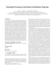
Beta(1,1) 

Beta(2,2) 

Beta(3,2) 

Beta(19,39) 

Figure 2: Several beta distributions. 

where h > 0and t > 0 are the parameters of the beta distribution, = h + t , and ;() 

is the Gamma function which satises ;(x +1)=x;(x) and ;(1) = 1. The quantities h 

and t are often referred to as hyperparameters to distinguish them from the parameter . 

The hyperparameters h and t must be greater than zero so that the distribution can be 

normalized. Examples of beta distributions are shown in Figure 2. 

The beta prior is convenient for several reasons. By Equation 3, the posterior distribution 

will also be a beta distribution: 

p(jD )= 

;( + N) 

;( h + h);( t + t) h+h;1 (1 ; ) t+t;1 =Beta(j h + h t + t) (6) 

We say that the set of beta distributions is a conjugate family of distributions for binomial 

sampling. Also, the expectation of with respect to this distribution has a simple form: 

Z 

Beta(j h t ) d = h 

 

Hence, given a beta prior, we have a simple expression for the probability of heads in the 

N + 1th toss: 

p(X N +1 = headsjD )= h + h 

(8) 

+ N 

Assuming p(j) is a beta distribution, it can be assessed in a number of ways. For 

example, we can assess our probability for heads in the rst toss of the thumbtack (e.g., 

using a probability wheel). Next, we can imagine having seen the outcomes of k ips, and 

reassess our probability for heads in the next toss. From Equation 8, we have (for k =1) 

p(X 1 = headsj) = 

h 

p(X 2 = headsjX 1 = heads ) = h +1 

h + t h + t +1 

Given these probabilities, we cansolvefor h and t . This assessment technique is known 

as the method of imagined future data. 

Another assessment method is based on Equation 6. This equation says that, if we start 

with a Beta(0 0) prior 4 and observe h heads and t tails, then our posterior (i.e., new 

4 Technically, the hyperparameters of this prior should be small positive numbers so that p(j) can be 

normalized. 

(7) 

7

prior) will be a Beta( h t ) distribution. Recognizing that a Beta(0 0) prior encodes a state 

of minimum information, we can assess h and t by determining the (possibly fractional) 

number of observations of heads and tails that is equivalent to our actual knowledge about 

ipping thumbtacks. Alternatively, we can assess p(X 1 = headsj) and, which can be 

regarded as an equivalent sample size for our current knowledge. This technique is known 

as the method of equivalent samples. Other techniques for assessing beta distributions are 

discussed by Winkler (1967) and Chaloner and Duncan (1983). 

Although the beta prior is convenient, it is not accurate for some problems. For example, 

suppose we think that the thumbtack mayhave been purchased at a magic shop. In this 

case, a more appropriate prior may be a mixture of beta distributions|for example, 

p(j) =0:4 Beta(20 1) + 0:4 Beta(1 20) + 0:2 Beta(2 2) 

where 0.4 is our probability that the thumbtack is heavily weighted toward heads (tails). 

In eect, we have introduced an additional hidden or unobserved variable H, whose states 

correspond to the three possibilities: (1) thumbtack is biased toward heads, (2) thumbtack 

is biased toward tails, and (3) thumbtack is normal and wehave asserted that conditioned 

on each state of H is a beta distribution. In general, there are simple methods (e.g., the 

method of imagined future data) for determining whether or not a beta prior is an accurate 

reection of one's beliefs. In those cases where the beta prior is inaccurate, an accurate 

prior can often be assessed by introducing additional hidden variables, as in this example. 

So far, we have only considered observations drawn from a binomial distribution. In 

general, observations may be drawn from any physical probability distribution: 

p(xj)=f(x ) 

where f(x ) is the likelihood function with parameters . For purposes of this discussion, 

we assume that the number of parameters is nite. As an example, X may be a continuous 

variable and have a Gaussian physical probability distribution with mean and variance v: 

p(xj)=(2v) ;1=2 e ;(x;)2 =2v 

where = f vg. 

Regardless of the functional form, we can learn about the parameters given data using 

the Bayesian approach. As we have done in the binomial case, we dene variables corresponding 

to the unknown parameters, assign priors to these variables, and use Bayes' rule 

to update our beliefs about these parameters given data: 

p(jD )= 

p(Dj) p(j) 

p(Dj) 

(9) 

8

We then average over the possible values of to make predictions. For example, 

p(x N+1 jD )= 

Z 

p(x N+1 j) p(jD ) d (10) 

For a class of distributions known as the exponential family, these computations can be 

done eciently and in closed form. 5 Members of this class include the binomial, multinomial, 

normal, Gamma, Poisson, and multivariate-normal distributions. Each member 

of this family has sucient statistics that are of xed dimension for any random sample, 

and a simple conjugate prior. 6 Bernardo and Smith (pp. 436{442, 1994) have compiled 

the important quantities and Bayesian computations for commonly used members of the 

exponential family. Here, we summarize these items for multinomial sampling, which we 

use to illustrate many of the ideas in this paper. 

In multinomial sampling, the observed variable X is discrete, having r possible states 

x 1 :::x r . The likelihood function is given by 

p(X = x k j)= k 

k =1:::r 

where = f 2 ::: r g are the parameters. (The parameter 1 is given by 1; P r 

k=2 k .) 

In this case, as in the case of binomial sampling, the parameters correspond to physical 

probabilities. The sucient statistics for data set D = fX 1 = x 1 :::X N = x N g are 

fN 1 :::N r g, where N i is the number of times X = x k in D. The simple conjugate prior 

used with multinomial sampling is the Dirichlet distribution: 

p(j) =Dir(j 1 ::: r ) 

;() 

Q rk=1 

;( k ) 

rY 

k=1 

k;1 

k 

(11) 

where = P r 

i=1 k , and k > 0k =1:::r. The posterior distribution p(jD ) = 

Dir(j 1 + N 1 ::: r + N r ). Techniques for assessing the beta distribution, including the 

methods of imagined future data and equivalent samples, can also be used to assess Dirichlet 

distributions. Given this conjugate prior and data set D, the probability distribution for 

the next observation is given by 

p(X N +1 = x k jD )= 

Z 

k Dir(j 1 + N 1 ::: r + N r ) d = k + N k 

+ N 

As we shall see, another important quantity inBayesian analysis is the marginal likelihood 

or evidence p(Dj). In this case, we have 

p(Dj)= 

;() 

;( + N) 

rY 

k=1 

;( k + N k ) 

;( k ) 

5 Recent advances in Monte-Carlo methods have made it possible to work eciently with many distributions 

outside the exponential family. See, for example, Gilks et al. (1996). 

6 In fact, except for a few, well-characterized exceptions, the exponential family is the only class of 

distributions that have sucient statistics of xed dimension (Koopman, 1936 Pitman, 1936). 

(12) 

(13) 

9

We note that the explicit mention of the state of knowledge is useful, because it reinforces 

the notion that probabilities are subjective. Nonetheless, once this concept is rmly in 

place, the notation simply adds clutter. In the remainder of this tutorial, we shall not 

mention explicitly. 

In closing this section, we emphasize that, although the Bayesian and classical approaches 

may sometimes yield the same prediction, they are fundamentally dierent methods 

for learning from data. As an illustration, let us revisit the thumbtack problem. Here, 

the Bayesian \estimate" for the physical probability of heads is obtained in a manner that 

is essentially the opposite of the classical approach. 

Namely, in the classical approach, is xed (albeit unknown), and we imagine all data 

sets of size N that may be generated by sampling from the binomial distribution determined 

by . Each datasetD will occur with some probability p(Dj) and will produce an estimate 

(D). To evaluate an estimator, we compute the expectation and variance of the estimate 

with respect to all such data sets: 

E p(Dj) ( ) = X D 

Var p(Dj) ( ) = X D 

p(Dj) (D) 

p(Dj) ( (D) ; E p(Dj) ( )) 2 (14) 

We then choose an estimator that somehow balances the bias ( ; E p(Dj) ( )) and variance 

of these estimates over the possible values for . 7 

Finally, we apply this estimator to the 

data set that we actually observe. A commonly-used estimator is the maximum-likelihood 

(ML) estimator, which selects the value of that maximizes the likelihood p(Dj). For 

binomial sampling, we have 

ML (D) = 

N k 

P rk=1 

N k 

For this (and other types) of sampling, the ML estimator is unbiased. That is, for all values 

of , the ML estimator has zero bias. In addition, for all values of , the variance of the 

ML estimator is no greater than that of any otherunbiased estimator (see, e.g., Schervish, 

1995). 

In contrast, in the Bayesian approach, D is xed, and we imagine all possible values of 

from which this data set could have been generated. Given , the \estimate" of the physical 

probability of heads is just itself. Nonetheless, we are uncertain about , and so our nal 

estimate is the expectation of with respect to our posterior beliefs about its value: 

E p(jD) () = 

Z 

p(jD ) d (15) 

7 Low biasandvariance are not the only desirable properties of an estimator. Other desirable properties 

include consistency and robustness. 

10

The expectations in Equations 14 and 15 are dierent and, in many cases, lead to 

dierent \estimates". One way to frame this dierence is to say that the classical and 

Bayesian approaches have dierent denitions for what it means to be a good estimator. 

Both solutions are \correct" in that they are self consistent. Unfortunately, both methods 

have their drawbacks, which has lead to endless debates about the merit of each approach. 

For example, Bayesians argue that it does not make sense to consider the expectations in 

Equation 14, because we only see a single data set. If we saw more than one data set, we 

should combine them into one larger data set. In contrast, classical statisticians argue that 

suciently accurate priors can not be assessed in many situations. The common view that 

seems to be emerging is that one should use whatever method that is most sensible for the 

task at hand. We share this view, although we alsobelieve that the Bayesian approach has 

been under used, especially in light of its advantages mentioned in the introduction (points 

three and four). Consequently, in this paper, we concentrate on the Bayesian approach. 

3 Bayesian Networks 

So far, we have considered only simple problems with one or a few variables. In real learning 

problems, however, we aretypically interested in looking for relationships among a large 

number of variables. The Bayesian network is a representation suited to this task. It is 

a graphical model that eciently encodes the joint probability distribution (physical or 

Bayesian) for a large set of variables. In this section, we dene a Bayesian network and 

show how one can be constructed from prior knowledge. 

ABayesian network for a set of variables X = fX 1 :::X n g consists of (1) a network 

structure S that encodes a set of conditional independence assertions about variables in X, 

and (2) a set P of local probability distributions associated with each variable. Together, 

these components dene the joint probability distribution for X. The network structure S is 

a directed acyclic graph. The nodes in S are in one-to-one correspondence with the variables 

X. WeuseX i to denote both the variable and its corresponding node, and Pa i to denote 

the parents of node X i in S as well as the variables corresponding to those parents. The 

lack of possible arcs in S encode conditional independencies. In particular, given structure 

S, the joint probability distribution for X is given by 

p(x)= 

nY 

i=1 

p(x i jpa i ) (16) 

The local probability distributions P are the distributions corresponding to the terms in 

the product of Equation 16. Consequently, the pair (S P ) encodes the joint distribution 

p(x). 

11

The probabilities encoded by aBayesian network may beBayesian or physical. When 

building Bayesian networks from prior knowledge alone, the probabilities will be Bayesian. 

When learning these networks from data, the probabilities will be physical (and their values 

may be uncertain). In subsequent sections, we describe how we can learn the structure and 

probabilities of a Bayesian network from data. In the remainder of this section, we explore 

the construction of Bayesian networks from prior knowledge. As we shall see in Section 10, 

this procedure can be useful in learning Bayesian networks as well. 

To illustrate the process of building a Bayesian network, consider the problem of detecting 

credit-card fraud. We begin by determining the variables to model. One possible 

choice of variables for our problem is Fraud (F ), Gas (G), Jewelry (J), Age (A), and Sex 

(S), representing whether or not the current purchase is fraudulent, whether or not there 

was a gas purchase in the last 24 hours, whether or not there was a jewelry purchase in 

the last 24 hours, and the age and sex of the card holder, respectively. The states of these 

variables are shown in Figure 3. Of course, in a realistic problem, we would include many 

more variables. Also, we could model the states of one or more of these variables at a ner 

level of detail. For example, we could let Age be a continuous variable. 

This initial task is not always straightforward. As part of this task we must (1) correctly 

identify the goals of modeling (e.g., prediction versus explanation versus exploration), (2) 

identify many possible observations that may be relevant to the problem, (3) determine what 

subset of those observations is worthwhile to model, and (4) organize the observations into 

variables having mutually exclusive and collectively exhaustive states. Diculties here are 

not unique to modeling with Bayesian networks, but rather are common to most approaches. 

Although there are no clean solutions, some guidance is oered by decision analysts (e.g., 

Howard and Matheson, 1983) and (when data are available) statisticians (e.g., Tukey, 1977). 

In the next phase of Bayesian-network construction, we build a directed acyclic graph 

that encodes assertions of conditional independence. One approach for doing so is based on 

the following observations. From the chain rule of probability, wehave 

p(x) = 

nY 

i=1 

p(x i jx 1 :::x i;1 ) (17) 

Now, for every X i , there will be some subset i fX 1 :::X i;1 g such that X i and 

fX 1 :::X i;1 gn i are conditionally independent given i . That is, for any x, 

p(x i jx 1 :::x i;1 )=p(x i j i ) (18) 

Combining Equations 17 and 18, we obtain 

p(x)= 

nY 

i=1 

12 

p(x i j i ) (19)

p(f=yes) = 0..00001 

Fraud 

p(a=

causal relationships among variables, and (2) causal relationships typically correspond to 

assertions of conditional dependence. In particular, to construct a Bayesian network for a 

given set of variables, we simply draw arcs from cause variables to their immediate eects. 

In almost all cases, doing so results in a network structure that satises the denition 

Equation 16. For example, given the assertions that Fraud is a direct cause of Gas, and 

Fraud, Age, and Sex are direct causes of Jewelry, we obtain the network structure in Figure 

3. The causal semantics of Bayesian networks are in large part responsible for the success 

of Bayesian networks as a representation for expert systems (Heckerman et al., 1995a). 

In Section 15, we will see how to learn causal relationships from data using these causal 

semantics. 

In the nal step of constructing a Bayesian network, we assess the local probability 

distribution(s) p(x i jpa i ). In our fraud example, where all variables are discrete, we assess 

one distribution for X i for every conguration of Pa i . Example distributions are shown in 

Figure 3. 

Note that, although we have described these construction steps as a simple sequence, 

they are often intermingled in practice. For example, judgments of conditional independence 

and/or cause and eect can inuence problem formulation. Also, assessments of probability 

can lead to changes in the network structure. Exercises that help one gain familiarity with 

the practice of building Bayesian networks can be found in Jensen (1996). 

4 Inference in a Bayesian Network 

Once we have constructed a Bayesian network (from prior knowledge, data, or a combination), 

we usually need to determine various probabilities of interest from the model. For 

example, in our problem concerning fraud detection, we want toknow the probability of 

fraud given observations of the other variables. This probability is not stored directly in 

the model, and hence needs to be computed. In general, the computation of a probability 

of interest given a model is known as probabilistic inference. In this section we describe 

probabilistic inference in Bayesian networks. 

Because a Bayesian network for X determines a joint probability distribution for X, we 

can|in principle|use the Bayesian network to compute any probability ofinterest. For 

example, from the Bayesian network in Figure 3, the probability of fraud given observations 

of the other variables can be computed as follows: 

p(fja s g j)= 

p(f a s g j) 

p(a s g j) 

= 

p(f a s g j) 

P 

f 0 p(f 0 asgj) 

(21) 

For problems with many variables, however, this direct approach is not practical. Fortu- 

14

nately, at least when all variables are discrete, we can exploit the conditional independencies 

encoded in a Bayesian network to make this computation more ecient. In our example, 

given the conditional independencies in Equation 20, Equation 21 becomes 

p(fja s g j) = 

= 

P 

f 0 

P 

f 0 

p(f)p(a)p(s)p(gjf)p(jjf a s) 

p(f 0 )p(a)p(s)p(gjf 0 )p(jjf 0 as) 

p(f)p(gjf)p(jjf a s) 

p(f 0 )p(gjf 0 )p(jjf 0 as) 

(22) 

Several researchers have developed probabilistic inference algorithms for Bayesian networks 

with discrete variables that exploit conditional independence roughly as we have 

described, although with dierent twists. For example, Howard and Matheson (1981), Olmsted 

(1983), and Shachter (1988) developed an algorithm that reverses arcs in the network 

structure until the answer to the given probabilistic query can be read directly from the 

graph. In this algorithm, each arc reversal corresponds to an application of Bayes' theorem. 

Pearl (1986) developed a message-passing scheme that updates the probability distributions 

for each nodeinaBayesian network in response to observations of one or more variables. 

Lauritzen and Spiegelhalter (1988), Jensen et al. (1990), and Dawid (1992) created an algorithm 

that rst transforms the Bayesian network into a tree where each node in the tree 

corresponds to a subset of variables in X. The algorithm then exploits several mathematical 

properties of this tree to perform probabilistic inference. Most recently, D'Ambrosio 

(1991) developed an inference algorithm that simplies sums and products symbolically, 

as in the transformation from Equation 21 to 22. The most commonly used algorithm for 

discrete variables is that of Lauritzen and Spiegelhalter (1988), Jensen et al (1990), and 

Dawid (1992). 

Methods for exact inference in Bayesian networks that encode multivariate-Gaussian or 

Gaussian-mixture distributions have beendeveloped by Shachter and Kenley (1989) and 

Lauritzen (1992), respectively. These methods also use assertions of conditional independence 

to simplify inference. Approximate methods for inference in Bayesian networks with 

other distributions, such as the generalized linear-regression model, have also been developed 

(Saul et al., 1996 Jaakkola and Jordan, 1996). 

Although we use conditional independence to simplify probabilistic inference, exact inference 

in an arbitrary Bayesian network for discrete variables is NP-hard (Cooper, 1990). 

Even approximate inference (for example, Monte-Carlo methods) is NP-hard (Dagum and 

Luby, 1993). The source of the diculty lies in undirected cycles in the Bayesian-network 

structure|cycles in the structure where we ignore the directionality of the arcs. (If we add 

an arc from Age to Gas in the network structure of Figure 3, then we obtain a structure with 

one undirected cycle: F ;G;A;J ;F .) When a Bayesian-network structure contains many 

15

undirected cycles, inference is intractable. For many applications, however, structures are 

simple enough (or can be simplied suciently without sacricing much accuracy) so that 

inference is ecient. For those applications where generic inference methods are impractical, 

researchers are developing techniques that are custom tailored to particular network 

topologies (Heckerman 1989 Suermondt and Cooper, 1991 Saul et al., 1996 Jaakkola and 

Jordan, 1996) or to particular inference queries (Ramamurthi and Agogino, 1988 Shachter 

et al., 1990 Jensen and Andersen, 1990 Darwiche and Provan, 1996). 

5 Learning Probabilities in a Bayesian Network 

In the next several sections, we showhow to rene the structure and local probability 

distributions of a Bayesian network given data. The result is set of techniques for data 

analysis that combines prior knowledge with data to produce improved knowledge. In 

this section, we consider the simplest version of this problem: using data to update the 

probabilities of a given Bayesian network structure. 

Recall that, in the thumbtack problem, we do not learn the probability of heads. Instead, 

we update our posterior distribution for the variable that represents the physical probability 

of heads. Wefollow the same approach for probabilities in a Bayesian network. In particular, 

we assume|perhaps from causal knowledge about the problem|that the physical joint 

probability distribution for X can be encoded in some network structure S. Wewrite 

p(xj s S h )= 

nY 

i=1 

p(x i jpa i i S h ) (23) 

where i is the vector of parameters for the distribution p(x i jpa i i S h ), s is the vector 

of parameters ( 1 ::: n ), and S h denotes the event (or \hypothesis" in statistics nomenclature) 

that the physical joint probability distribution can be factored according to S. 8 In 

addition, we assume that we have a random sample D = fx 1 :::x N g from the physical 

joint probability distribution of X. We refer to an element x l of D as a case. As in Section 2, 

we encode our uncertainty about the parameters s by dening a (vector-valued) variable 

s , and assessing a prior probability density function p( s jS h ). The problem of learning 

probabilities in a Bayesian network can now be stated simply: Given a random sample D, 

compute the posterior distribution p( s jD S h ). 

8 As dened here, network-structure hypotheses overlap. For example, given X = fX 1X 2g, any joint 

distribution for X that can be factored according the network structure containing no arc, can also be 

factored according to the network structure X 1 ;! X 2. Such overlap presents problems for model averaging, 

described in Section 7. Therefore, we should add conditions to the denition to insure no overlap. Heckerman 

and Geiger (1996) describe one such set of conditions. 

16

We refer to the distribution p(x i jpa i i S h ), viewed as a function of i ,asalocal distribution 

function. Readers familiar with methods for supervised learning will recognize that 

a local distribution function is nothing more than a probabilistic classication or regression 

function. Thus,aBayesian network can be viewed as a collection of probabilistic classication/regression 

models, organized by conditional-independence relationships. Examples of 

classication/regression models that produce probabilistic outputs include linear regression, 

generalized linear regression, probabilistic neural networks (e.g., MacKay, 1992a, 1992b), 

probabilistic decision trees (e.g., Buntine, 1993 Friedman and Goldszmidt, 1996), kernel 

density estimation methods (Book, 1994), and dictionary methods (Friedman, 1995). In 

principle, any of these forms can be used to learn probabilities in a Bayesian network and, 

in most cases, Bayesian techniques for learning are available. Nonetheless, the most studied 

models include the unrestricted multinomial distribution (e.g., Cooper and Herskovits, 

1992), linear regression with Gaussian noise (e.g., Buntine, 1994 Heckerman and Geiger, 

1996), and generalized linear regression (e.g., MacKay, 1992a and 1992b Neal, 1993 and 

Saul et al., 1996). 

In this tutorial, we illustrate the basic ideas for learning probabilities (and structure) 

using the unrestricted multinomial distribution. In this case, each variable X i 2 X is discrete, 

having r i possible values x 1 i :::xr i 

i , and each local distribution function is collection 

of multinomial distributions, one distribution for each conguration of Pa i . Namely, we 

assume 

where pa 1 i :::paq i 

i 

p(x k i jpa j i iS h )= ijk > 0 (24) 

(q i = Q X i 2Pa i 

r i ) denote the congurations of Pa i ,and i =(( ijk ) r i 

k=2 )q i 

j=1 

are the parameters. (The parameter ij1 is given by 1; P r i 

k=2 ijk.) For convenience, we 

dene the vector of parameters 

ij =( ij2 ::: ijri ) 

for all i and j. We use the term \unrestricted" to contrast this distribution with multinomial 

distributions that are low-dimensional functions of Pa i |for example, the generalized linearregression 

model. 

Given this class of local distribution functions, we can compute the posterior distribution 

p( s jD S h ) eciently and in closed form under two assumptions. The rst assumption is 

that there are no missing data in the random sample D. Wesay that the random sample 

D is complete. The second assumption is that the parameter vectors ij are mutually 

17

Θ x 

Θ y|x 

Θ y|x 

X 

Y 

sample 1 

X 

Y 

 

sample 2 

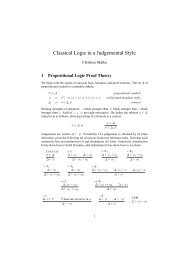
Figure 4: A Bayesian-network structure depicting the assumption of parameter independence 

for learning the parameters of the network structure X ! Y . Both variables X and 

Y are binary. Weusex and x to denote the two statesofX, andy and y to denote the two 

states of Y . 

independent. 9 That is, 

p( s jS h )= 

nY 

Yq i 

i=1 j=1 

p( ij jS h ) 

We refer to this assumption, which was introduced by Spiegelhalter and Lauritzen (1990), 

as parameter independence. 

Given that the joint physical probability distribution factors according to some network 

structure S, the assumption of parameter independence can itself be represented by a larger 

Bayesian-network structure. For example, the network structure in Figure 4 represents the 

assumption of parameter independence for X = fX Y g (X, Y binary) and the hypothesis 

that the network structure X ! Y encodes the physical joint probability distribution for 

X. 

Under the assumptions of complete data and parameter independence, the parameters 

remain independent given a random sample: 

p( s jD S h )= 

nY 

Yq i 

i=1 j=1 

p( ij jD S h ) (25) 

Thus, we can update each vector of parameters ij independently, just as in the one-variable 

case. Assuming each vector ij has the prior distribution Dir( ij j ij1 ::: ijri ), we obtain 

9 The computation is also straightforward if two or more parameters are equal. For details, see Thiesson 

(1995). 

18

the posterior distribution 

p( ij jD S h ) = Dir( ij j ij1 + N ij1 ::: ijri + N ijri ) (26) 

where N ijk is the number of cases in D in which X i = x k i and Pa i = pa j i . 

As in the thumbtack example, we canaverage over the possible congurations of s to 

obtain predictions of interest. For example, let us compute p(x N+1 jD S h ), where x N+1 is 

the next case to be seen after D. Suppose that, in case x N+1 , X i = x k i and Pa i = pa j i , 

where k and j depend on i. Thus, 

p(x N +1 jD S h )=E p(sjDS h ) 

nY 

i=1 

ijk 

! 

To compute this expectation, we rst use the fact that the parameters remain independent 

given D: 

p(x N +1 jD S h )= 

Z n Y 

i=1 

Then, we use Equation 12 to obtain 

ijk p( s jD S h ) d s = 

p(x N +1 jD S h )= 

nY 

i=1 

nY Z 

i=1 

ijk p( ij jD S h ) d ij 

ijk + N ijk 

ij + N ij 

(27) 

where ij = P r i 

k=1 ijk and N ij = P r i 

k=1 N ijk. 

These computations are simple because the unrestricted multinomial distributions are in 

the exponential family. Computations for linear regression with Gaussian noise are equally 

straightforward (Buntine, 1994 Heckerman and Geiger, 1996). 

6 Methods for Incomplete Data 

Let us now discuss methods for learning about parameters when the random sample is 

incomplete (i.e., some variables in some cases are not observed). An important distinction 

concerning missing data is whether or not the absence of an observation is dependent on the 

actual states of the variables. For example, a missing datum in a drug study may indicate 

that a patient became too sick|perhaps due to the side eects of the drug|to continue 

in the study. In contrast, if a variable is hidden (i.e., never observed in any case), then 

the absence of this data is independent of state. Although Bayesian methods and graphical 

models are suited to the analysis of both situations, methods for handling missing data 

where absence is independent of state are simpler than those where absence and state are 

dependent. In this tutorial, we concentrate on the simpler situation only. Readers interested 

in the more complicated case should see Rubin (1978), Robins (1986), and Pearl (1995). 

19

Continuing with our example using unrestricted multinomial distributions, suppose we 

observe a single incomplete case. Let Y X and Z X denote the observed and unobserved 

variables in the case, respectively. Under the assumption of parameter independence, 

we can compute the posterior distribution of ij for network structure S as follows: 

p( ij jyS h )= X z 

p(zjyS h ) p( ij jy zS h ) (28) 

n o 

=(1; p(pa j i jySh )) p( ij jS h ) + 

Xr i 

k=1 

n 

o 

p(x k i paj i jySh ) p( ij jx k i paj i Sh ) 

(See Spiegelhalter and Lauritzen (1990) for a derivation.) Each term in curly brackets in 

Equation 28 is a Dirichlet distribution. Thus, unless both X i and all the variables in Pa i are 

observed in case y, the posterior distribution of ij will be a linear combination of Dirichlet 

distributions|that is, a Dirichlet mixture with mixing coecients (1 ; p(pa j i jySh )) and 

p(x k i paj i jySh )k=1:::r i . 

When we observe a second incomplete case, some or all of the Dirichlet components 

in Equation 28 will again split into Dirichlet mixtures. That is, the posterior distribution 

for ij we become a mixture of Dirichlet mixtures. As we continue to observe incomplete 

cases, each missing values for Z, the posterior distribution for ij will contain a number of 

components that is exponential in the number of cases. In general, for any interesting set 

of local likelihoods and priors, the exact computation of the posterior distribution for s 

will be intractable. Thus, we require an approximation for incomplete data. 

6.1 Monte-Carlo Methods 

One class of approximations is based on Monte-Carlo or sampling methods. These approximations 

can be extremely accurate, provided one is willing to wait long enough for the 

computations to converge. 

In this section, we discuss one of many Monte-Carlo methods known as Gibbs sampling, 

introduced by Geman and Geman (1984). Given variables X = fX 1 :::X n g with some 

joint distribution p(x), we can use a Gibbs sampler to approximate the expectation of a 

function f(x) with respect to p(x) as follows. First, we choose an initial state for each of 

the variables in X somehow (e.g., at random). Next, we pick somevariable X i , unassign 

its current state, and compute its probability distribution given the states of the other 

n ; 1variables. Then, we sample a state for X i based on this probability distribution, and 

compute f(x). Finally, we iterate the previous two steps, keeping track of the average value 

of f(x). In the limit, as the number of cases approach innity, this average is equal to 

E p(x) (f(x)) provided two conditions are met. First, the Gibbs sampler must be irreducible: 

20

The probability distribution p(x) must be such thatwe can eventually sample any possible 

conguration of X given any possible initial conguration of X. 

contains no zero probabilities, then the Gibbs sampler will be irreducible. 

For example, if p(x) 

Second, each 

X i must be chosen innitely often. In practice, an algorithm for deterministically rotating 

through the variables is typically used. Introductions to Gibbs sampling and other Monte- 

Carlo methods|including methods for initialization and a discussion of convergence|are 

given by Neal (1993) and Madigan and York (1995). 

To illustrate Gibbs sampling, let us approximate the probability density p( s jD S h ) for 

some particular conguration of s ,given an incomplete data set D = fy 1 :::y N g and a 

Bayesian network for discrete variables with independent Dirichlet priors. To approximate 

p( s jD S h ), we rst initialize the states of the unobserved variables in each case somehow. 

As a result, we have a complete random sample D c . Second, we choose some variable X il 

(variable X i in case l) that is not observed in the original random sample D, and reassign 

its state according to the probability distribution 

p(x 0 iljD c n x il S h )= p(x0 il D c n x il jS h ) 

P 

p(x 00 

il D c n x il jS h ) 

where D c n x il denotes the data set D c with observation x il removed, and the sum in the 

denominator runs over all states of variable X il . As we shall see in Section 7, the terms 

in the numerator and denominator can be computed eciently (see Equation 35). Third, 

we repeat this reassignment for all unobserved variables in D, producing a new complete 

random sample D 0 c.Fourth, we compute the posterior density p( s jD 0 cS h ) as described in 

Equations 25 and 26. Finally, we iterate the previous three steps, and use the average of 

p( s jD 0 cS h ) as our approximation. 

6.2 The Gaussian Approximation 

Monte-Carlo methods yield accurate results, but they are often intractable|for example, 

when the sample size is large. Another approximation that is more ecient than Monte- 

Carlo methods and often accurate for relatively large samples is the Gaussian approximation 

(e.g., Kass et al., 1988 Kass and Raftery, 1995). 

x 00 

il 

The idea behind this approximation is that, for large amounts of data, p( s jD S h ) 

/ p(Dj s S h )p( s jS h ) can often be approximated as a multivariate-Gaussian distribution. 

In particular, let 

g( s ) log(p(Dj s S h ) p( s jS h )) (29) 

Also, dene ~ s to be the conguration of s that maximizes g( s ). This conguration also 

maximizes p( s jD S h ), and is known as the maximum a posteriori (MAP) conguration of 

21

s . Using a second degree Taylor polynomial of g( s ) about the ~ s to approximate g( s ), 

we obtain 

g( s ) g( ~ s ) ; 1 2 ( s ; ~ s )A( s ; ~ s ) t (30) 

where ( s ; ~ s ) t is the transpose of row vector ( s ; ~ s ), and A is the negative Hessian of 

g( s )evaluated at ~ s . Raising g( s ) to the power of e and using Equation 29, we obtain 

p( s jD S h ) / p(Dj s S h ) p( s jS h ) (31) 

 

p(Dj ~ s S h ) p( ~ s jS h )expf; 1 2 ( s ; ~ s )A( s ; ~ s ) t g 

Hence, p( s jD S h ) is approximately Gaussian. 

To compute the Gaussian approximation, we must compute ~ s as well as the negative 

Hessian of g( s )evaluated at ~ s . In the following section, we discuss methods for nding 

~ s . Meng and Rubin (1991) describe a numerical technique for computing the second 

derivatives. Raftery (1995) shows how toapproximate the Hessian using likelihood-ratio 

tests that are available in many statistical packages. Thiesson (1995) demonstrates that, 

for unrestricted multinomial distributions, the second derivatives can be computed using 

Bayesian-network inference. 

6.3 The MAP and ML Approximations and the EM Algorithm 

As the sample size of the data increases, the Gaussian peak will become sharper, tending 

to a delta function at the MAP conguration ~ s . In this limit, we do not need to compute 

averages or expectations. 

conguration. 

Instead, we simply make predictions based on the MAP 

A further approximation is based on the observation that, as the sample size increases, 

the eect of the prior p( s jS h ) diminishes. Thus, we can approximate ~ s by the maximum 

maximum likelihood (ML) conguration of s : 

^ s = arg max 

s 

n 

p(Dj s S h ) 

One class of techniques for nding a ML or MAP is gradient-based optimization. For 

example, we can use gradient ascent, where we follow the derivatives of g( s ) or the likelihood 

p(Dj s S h ) to a local maximum. Russell et al. (1995) and Thiesson (1995) show 

how to compute the derivatives of the likelihood for a Bayesian network with unrestricted 

multinomial distributions. Buntine (1994) discusses the more general case where the likelihood 

function comes from the exponential family. Of course, these gradient-based methods 

nd only local maxima. 

o 

22

Another technique for nding a local ML or MAP is the expectation{maximization (EM) 

algorithm (Dempster et al., 1977). To ndalocalMAPorML,we begin by assigning a 

conguration to s somehow (e.g., at random). Next, we compute the expected sucient 

statistics for a complete data set, where expectation is taken with respect to the joint 

distribution for X conditioned on the assigned conguration of s and the known data D. 

In our discrete example, we compute 

E p(xjDsS h )(N ijk )= 

NX 

l=1 

p(x k i pa j i jy l s S h ) (32) 

where y l is the possibly incomplete lth case in D. When X i and all the variables in Pa i 

are observed in case x l , the term for this case requires a trivial computation: it is either 

zero or one. Otherwise, we can use any Bayesian network inference algorithm to evaluate 

the term. This computation is called the expectation step of the EM algorithm. 

Next, we use the expected sucient statistics as if they were actual sucient statistics 

from a complete random sample D c .Ifwe are doing an ML calculation, then we determine 

the conguration of s that maximize p(D c j s S h ). In our discrete example, we have 

ijk = 

E p(xjDsS h )(N ijk ) 

P ri 

k=1 E p(xjD sS h )(N ijk ) 

If we are doing a MAP calculation, then we determine the conguration of s that maximizes 

p( s jD c S h ). In our discrete example, we have 10 

ijk = 

ijk +E p(xjDsS )(N h ijk ) 

P ri 

k=1 ( ijk +E p(xjDsS )(N h ijk )) 

This assignment is called the maximization step of the EM algorithm. Dempster et al. 

(1977) showed that, under certain regularity conditions, iteration of the expectation and 

maximization steps will converge to a local maximum. The EM algorithm is typically 

applied when sucient statistics exist (i.e., when local distribution functions are in the 

exponential family), although generalizations of the EM algroithm have been used for more 

complicated local distributions (see, e.g., Saul et al. 1996). 

10 The MAP conguration s 

~ depends on the coordinate system in which the parameter variables are 

expressed. The expression for the MAP conguration given here is obtained by the following procedure. First, 

we transform each variable set ij =( ij2::: ijri ) to the new coordinate system ij =( ij2::: ijri ), 

where ijk = log( ijk= ij1)k =2:::r i. This coordinate system, which we denote by s, is sometimes 

referred to as the canonical coordinate system for the multinomial distribution (see, e.g., Bernardo and Smith, 

1994, pp. 199{202). Next, we determine the conguration of s that maximizes p( sjD cS h ). Finally, 

we transform this MAP conguration to the original coordinate system. Using the MAP conguration 

corresponding to the coordinate system s has several advantages, which are discussed in Thiesson (1995b) 

and MacKay (1996). 

23

7 Learning Parameters and Structure 

Now we consider the problem of learning about both the structure and probabilities of a 

Bayesian network given data. 

Assuming we think structure can be improved, we must be uncertain about the network 

structure that encodes the physical joint probability distribution for X. 

Following the 

Bayesian approach, we encode this uncertainty by dening a (discrete) variable whose states 

correspond to the possible network-structure hypotheses S h , and assessing the probabilities 

p(S h ). Then, given a random sample D from the physical probability distribution for X, 

we compute the posterior distribution p(S h jD) and the posterior distributions p( s jD S h ), 

and use these distributions in turn to compute expectations of interest. For example, to 

predict the next case after seeing D, we compute 

p(x N +1 jD) = X S h 

p(S h jD) 

Z 

p(x N+1 j s S h ) p( s jD S h ) d s (33) 

In performing the sum, we assume that the network-structure hypotheses are mutually 

exclusive. We return to this point in Section 9. 

The computation of p( s jD S h )isaswehave described in the previous two sections. 

The computation of p(S h jD) is also straightforward, at least in principle. 

theorem, we have 

From Bayes' 

p(S h jD) =p(S h ) p(DjS h )=p(D) (34) 

where p(D) is a normalization constant that does not depend upon structure. Thus, to determine 

the posterior distribution for network structures, we need to compute the marginal 

likelihood of the data (p(DjS h )) for each possible structure. 

We discuss the computation of marginal likelihoods in detail in Section 9. As an introduction, 

consider our example with unrestricted multinomial distributions, parameter 

independence, Dirichlet priors, and complete data. As we have discussed, when there are 

no missing data, each parameter vector ij is updated independently. In eect, we have 

a separate multi-sided thumbtack problem for every i and j. Consequently, the marginal 

likelihood of the data is the just the product of the marginal likelihoods for each i{j pair 

(given by Equation 13): 

p(DjS h )= 

nY 

Yq i 

i=1 j=1 

;( ij ) Yr i 

;( ij + N ij ) 

k=1 

;( ijk + N ijk ) 

;( ijk ) 

This formula was rst derived by Cooper and Herskovits (1992). 

Unfortunately, the full Bayesian approach that we have described is often impractical. 

One important computation bottleneck is produced by the average over models in Equation 

33. If we consider Bayesian-network models with n variables, the number of possible 

24 

(35)

structure hypotheses is more than exponential in n. Consequently, in situations where the 

user can not exclude almost all of these hypotheses, the approach isintractable. 

Statisticians, who have been confronted by this problem for decades in the context of 

other types of models, use two approaches to address this problem: model selection and 

selective model averaging. The former approach is to select a \good" model (i.e., structure 

hypothesis) from among all possible models, and use it as if it were the correct model. The 

latter approach is to select a manageable number of good models from among all possible 

models and pretend that these models are exhaustive. These related approaches raise several 

important questions. In particular, do these approaches yield accurate results when applied 

to Bayesian-network structures? If so, how dowe search for good models? And how dowe 

decide whether or not a model is \good"? 

The question of accuracy is dicult to answer in theory. Nonetheless, several researchers 

have shown experimentally that the selection of a single good hypothesis often yields accurate 

predictions (Cooper and Herskovits 1992 Aliferis and Cooper 1994 Heckerman et 

al., 1995b) and that model averaging using Monte-Carlo methods can sometimes be ecient 

and yield even better predictions (Madigan et al., 1996). These results are somewhat 

surprising, and are largely responsible for the great deal of recent interest in learning with 

Bayesian networks. In Sections 8 through 10, we consider dierent denitions of what is 

means for a model to be \good", and discuss the computations entailed by some of these 

denitions. In Section 11, we discuss model search. 

We note that model averaging and model selection lead to models that generalize well to 

new data. That is, these techniques help us to avoid the overtting of data. As is suggested 

by Equation 33, Bayesian methods for model averaging and model selection are ecient in 

the sense that all cases in D can be used to both smooth and train the model. As we shall 

see in the following two sections, this advantage holds true for the Bayesian approach in 

general. 

8 Criteria for Model Selection 

Most of the literature on learning with Bayesian networks is concerned with model selection. 

In these approaches, some criterion is used to measure the degree to which a network 

structure (equivalence class) ts the prior knowledge and data. A search algorithm is then 

used to nd an equivalence class that receives a high score by this criterion. Selective model 

averaging is more complex, because it is often advantageous to identify network structures 

that are signicantly dierent. In many cases, a single criterion is unlikely to identify 

such complementary network structures. In this section, we discuss criteria for the simpler 

25

problem of model selection. For a discussion of selective modelaveraging, see Madigan and 

Raftery (1994). 

8.1 Relative Posterior Probability 

A criterion that is often used for model selection is the log of the relative posterior probability 

log p(D S h )=logp(S h )+logp(DjS h ). 11 The logarithm is used for numerical convenience. 

This criterion has two components: the log prior and the log marginal likelihood. 

In Section 9, we examine the computation of the log marginal likelihood. In Section 10.2, 

we discuss the assessment ofnetwork-structure priors. Note that our comments about these 

terms are also relevant to the full Bayesian approach. 

The log marginal likelihood has the following interesting interpretation described by 

Dawid (1984). From the chain rule of probability, wehave 

log p(DjS h )= 

NX 

l=1 

log p(x l jx 1 :::x l;1 S h ) (36) 

The term p(x l jx 1 :::x l;1 S h ) is the prediction for x l made by modelS h after averaging 

over its parameters. The log of this term can be thought of as the utility or reward for this 

prediction under the utility function log p(x). 12 Thus, a model with the highest log marginal 

likelihood (or the highest posterior probability, assuming equal priors on structure) is also 

a model that is the best sequential predictor of the data D under the log utility function. 

Dawid (1984) also notes the relationship between this criterion and cross validation. 

When using one form of cross validation, known as leave-one-out cross validation, 

we rst train a model on all but one of the cases in the random sample|say, 

V l = fx 1 :::x l;1 x l+1 :::x N g. Then, we predict the omitted case, and reward this prediction 

under some utility function. Finally, we repeat this procedure for every case in the 

random sample, and sum the rewards for each prediction. If the prediction is probabilistic 

and the utility function is log p(x), we obtain the cross-validation criterion 

CV(S h D)= 

NX 

l=1 

log p(x l jV l S h ) (37) 

which is similar to Equation 36. One problem with this criterion is that training and test 

cases are interchanged. For example, when we compute p(x 1 jV 1 S h ) in Equation 37, we use 

11 An equivalent criterion that is often used is log(p(S h jD)=p(S h 0 jD)) = log(p(S h )=p(S h 0 )) + 

log(p(DjS h )=p(DjS h 0 )). The ratio p(DjS h )=p(DjS h 0 ) is known as a Bayes' factor. 

12 This utility function is known as a proper scoring rule, because its use encourages people to assess their 

true probabilities. Foracharacterization of proper scoring rules and this rule in particular, see Bernardo 

(1979). 

26

x 2 for training and x 1 for testing. Whereas, when we compute p(x 2 jV 2 S h ), we usex 1 for 

training and x 2 for testing. Such interchanges can lead to the selection of a model that over 

ts the data (Dawid, 1984). Various approaches for attenuating this problem have been 

described, but we see from Equation 36 that the log-marginal-likelihood criterion avoids 

the problem altogether. Namely, when using this criterion, we never interchange training 

and test cases. 

8.2 Local Criteria 

Consider the problem of diagnosing an ailment given the observation of a set of ndings. 

Suppose that the set of ailments under consideration are mutually exclusive and collectively 

exhaustive, so that we may represent these ailments using a single variable A. A possible 

Bayesian network for this classication problem is shown in Figure 5. 

The posterior-probability criterion is global in the sense that it is equally sensitive toall 

possible dependencies. In the diagnosis problem, the posterior-probability criterion is just 

as sensitive to dependencies among the nding variables as it is to dependencies between 

ailment and ndings. Assuming that we observe all (or perhaps all but a few) of the ndings 

in D, a more reasonable criterion would be local in the sense that it ignores dependencies 

among ndings and is sensitive only to the dependencies among the ailment and ndings. 

This observation applies to all classication and regression problems with complete data. 

One such local criterion, suggested by Spiegelhalter et al. (1993), is a variation on the 

sequential log-marginal-likelihood criterion: 

LC(S h D)= 

NX 

l=1 

log p(a l jF l D l S h ) (38) 

where a l and F l denote the observation of the ailment A and ndings F in the lth case, 

respectively. In other words, to compute the lth term in the product, we train our model 

S with the rst l ; 1 cases, and then determine how well it predicts the ailment given the 

ndings in the lth case. We can view this criterion, like the log-marginal-likelihood, as a 

form of cross validation where training and test cases are never interchanged. 

The log utility function has interesting theoretical properties, but it is sometimes inaccurate 

for real-world problems. In general, an appropriate reward or utility function will 

depend on the decision-making problem or problems to which the probabilistic models are 

applied. Howard and Matheson (1983) have collected a series of articles describing how 

to construct utility models for specic decision problems. Once we construct such utility 

models, we can use suitably modied forms of Equation 38 for model selection. 

27

Ailment 

Finding 1 

. . . 

Finding n 

Finding 2 

Figure 5: A Bayesian-network structure for medical diagnosis. 

9 Computation of the Marginal Likelihood 

As mentioned, an often-used criterion for model selection is the log relative posterior probability 

log p(D S h )=logp(S h ) + log p(DjS h ). In this section, we discuss the computation 

of the second component of this criterion: the log marginal likelihood. 

Given (1) local distribution functions in the exponential family, (2)mutual independence 

of the parameters i , (3) conjugate priors for these parameters, and (4) complete data, the 

log marginal likelihood can be computed eciently and in closed form. Equation 35 is an 

example for unrestricted multinomial distributions. 

Buntine (1994) and Heckerman and 

Geiger (1996) discuss the computation for other local distribution functions. 

concentrate on approximations for incomplete data. 

Here, we 

The Monte-Carlo and Gaussian approximations for learning about parameters that we 

discussed in Section 6 are also useful for computing the marginal likelihood given incomplete 

data. One Monte-Carlo approach, described by Chib (1995) and Raftery (1996), uses Bayes' 

theorem: 

p(DjS h )= p( sjS h ) p(Dj s S h ) 

p( s jD S h ) 

For any conguration of s , the prior term in the numerator can be evaluated directly. In 

addition, the likelihood term in the numerator can be computed using Bayesian-network 

inference. 

(39) 

Finally, the posterior term in the denominator can be computed using Gibbs 

sampling, as we described in Section 6.1. Other, more sophisticated Monte-Carlo methods 

are described by DiCiccio et al. (1995). 

As we have discussed, Monte-Carlo methods are accurate but computationally inecient, 

especially for large databases. In contrast, methods based on the Gaussian approximation 

are more ecient, and can be as accurate as Monte-Carlo methods on large data 

sets. 

Recall that, for large amounts of data, p(Dj s S h ) p( s jS h ) can often be approximated 

28

asamultivariate-Gaussian distribution. Consequently, 

p(DjS h )= 

Z 

p(Dj s S h ) p( s jS h ) d s (40) 

can be evaluated in closed form. In particular, substituting Equation 31 into Equation 40, 

integrating, and taking the logarithm of the result, we obtain the approximation: 

log p(DjS h ) log p(Dj ~ s S h ) + log p( ~ s jS h ) + d 2 log(2) ; 1 log jAj (41) 

2 

where d is the dimension of g( s ). For a Bayesian network with unrestricted multinomial 

distributions, this dimension is typically given by P n 

i=1 q i (r i ; 1). Sometimes, when there 

are hidden variables, this dimension is lower. See Geiger et al. (1996) for a discussion of 

this point. 

This approximation technique for integration is known as Laplace's method, and we refer 

to Equation 41 as the Laplace approximation. Kass et al. (1988) have shown that, under 

certain regularity conditions, relative errors in this approximation are O(1=N), where N is 

the number of cases in D. Thus, the Laplace approximation can be extremely accurate. 

For more detailed discussions of this approximation, see|for example|Kass et al. (1988) 

and Kass and Raftery (1995). 

Although Laplace's approximation is ecient relative toMonte-Carlo approaches, the 

computation of jAj is nevertheless intensive for large-dimension models. One simplication 

is to approximate jAj using only the diagonal elements of the Hessian A. Although in so 

doing, we incorrectly impose independencies among the parameters, researchers have shown 

that the approximation can be accurate in some circumstances (see, e.g., Becker and Le 

Cun, 1989, and Chickering and Heckerman, 1996). Another ecient variant of Laplace's 

approximation is described by Cheeseman and Stutz (1995), who use the approximation in 

the AutoClass program for data clustering (see also Chickering and Heckerman, 1996.) 

We obtain a very ecient (but less accurate) approximation by retaining only those 

terms in Equation 41 that increase with N: logp(Dj ~ s S h ), which increases linearly with 

N, and log jAj, which increases as d log N. Also, for large N, s ~ can be approximated by 

the ML conguration of s .Thus, we obtain 

log p(DjS h ) log p(Dj ^ s S h ) ; d log N (42) 

2 

This approximation is called the Bayesian information criterion (BIC), and was rst derived 

by Schwarz (1978). 

The BIC approximation is interesting in several respects. First, it does not depend on 

the prior. Consequently, we can use the approximation without assessing a prior. 13 Sec- 

13 One of the technical assumptions used to derive this approximation is that the prior is non-zero around 

^ s. 

29

ond, the approximation is quite intuitive. Namely, itcontains a term measuring how well 

the parameterized model predicts the data (log p(Dj ^ s S h )) and a term that punishes the 

complexity of the model (d=2 logN). Third, the BIC approximation is exactly minus the 

Minimum Description Length (MDL) criterion described by Rissanen (1987). Thus, recalling 

the discussion in Section 9, we see that the marginal likelihood provides a connection 

between cross validation and MDL. 

10 Priors 

To compute the relative posterior probability ofanetwork structure, we must assess the 

structure prior p(S h ) and the parameter priors p( s jS h ) (unless we are using large-sample 

approximations such as BIC/MDL). The parameter priors p( s jS h ) are also required for 

the alternative scoring functions discussed in Section 8. Unfortunately, when many network 

structures are possible, these assessments will be intractable. Nonetheless, under certain 

assumptions, we can derive the structure and parameter priors for many network structures 

from a manageable number of direct assessments. Several authors have discussed such 

assumptions and corresponding methods for deriving priors (Cooper and Herskovits, 1991, 

1992 Buntine, 1991 Spiegelhalter et al., 1993 Heckerman et al., 1995b Heckerman and 

Geiger, 1996). In this section, we examine some of these approaches. 

10.1 Priors on Network Parameters 

First, let us consider the assessment of priors for the parameters of network structures. 

We consider the approach ofHeckerman et al. (1995b) who address the case where the 

local distribution functions are unrestricted multinomial distributions and the assumption 

of parameter independence holds. 

Their approach is based on twokey concepts: independence equivalence and distribution 

equivalence. Wesay that twoBayesian-network structures for X are independenceequivalent 

if they represent the same set of conditional-independence assertions for X (Verma and 

Pearl, 1990). For example, given X = fX Y Zg, the network structures X ! Y ! Z, 

X Y ! Z, and X Y Z represent only the independence assertion that X and Z are 

conditionally independent given Y . Consequently, these network structures are equivalent. 

As another example, a complete network structure is one that has no missing edge|that is, 

it encodes no assertion of conditional independence. When X contains n variables, there are 

n! possible complete network structures: one network structure for each possible ordering 

of the variables. All complete network structures for p(x) are independence equivalent. In 

general, two network structures are independence equivalent if and only if they have the 

30

same structure ignoring arc directions and the same v-structures (Verma and Pearl, 1990). 

A v-structure is an ordered tuple (X Y Z) such that there is an arc from X to Y and from 

Z to Y , but no arc between X and Z. 

The concept of distribution equivalence is closely related to that of independence equivalence. 

Suppose that all Bayesian networks for X under consideration have local distribution 

functions in the family F. This is not a restriction, per se, because F can be a large family. 

We say that two Bayesian-network structures S 1 and S 2 for X are distribution equivalent 

with respect to (wrt) F if they represent the same joint probability distributions for X|that 

is, if, for every s1 , there exists a s2 such that p(xj s1 S1 h )=p(xj s2 S2 h ), and vice versa. 

Distribution equivalence wrt some F implies independence equivalence, but the converse 

does not hold. For example, when F is the family of generalized linear-regression 

models, the complete network structures for n 3variables do not represent the same 

sets of distributions. Nonetheless, there are families F|for example, unrestricted multinomial 

distributions and linear-regression models with Gaussian noise|where independence 

equivalence implies distribution equivalence wrt F (Heckerman and Geiger, 1996). 

The notion of distribution equivalence is important, because if two network structures 

S 1 and S 2 are distribution equivalent wrt to a given F, then the hypotheses associated with 

these two structures are identical|that is, S1 h = S2 h . Thus, for example, if S 1 and S 2 are 

distribution equivalent, then their probabilities must be equal in any state of information. 

Heckerman et al. (1995b) call this property hypothesis equivalence. 

In light of this property, we should associate each hypothesis with an equivalence class 

of structures rather than a single network structure, and our methods for learning network 

structure should actually be interpreted as methods for learning equivalence classes of network 

structures (although, for the sake of brevity, we often blur this distinction). Thus, 

for example, the sum over network-structure hypotheses in Equation 33 should be replaced 

with a sum over equivalence-class hypotheses. An ecient algorithm for identifying the 

equivalence class of a given network structure can be found in Chickering (1995). 

We note that hypothesis equivalence holds provided we interpret Bayesian-network 

structure simply as a representation of conditional independence. Nonetheless, stronger definitions 

of Bayesian networks exist where arcs have a causal interpretation (see Section 15). 

Heckerman et al. (1995b) and Heckerman (1995) argue that, although it is unreasonable 

to assume hypothesis equivalence when working with causal Bayesian networks,itisoften 

reasonable to adopt a weaker assumption of likelihood equivalence, which says that the 

observations in a database can not help to discriminate two equivalent network structures. 

Now let us return to the main issue of this section: the derivation of priors from a manageable 

number of assessments. Geiger and Heckerman (1995) show that the assumptions 

31

of parameter independence and likelihood equivalence imply that the parameters for any 

complete network structure S c must have a Dirichlet distribution with constraints on the 

hyperparameters given by 

ijk = p(x k i pa j i jSh c ) (43) 

where is the user's equivalent sample size, 14 ,andp(x k i paj i jSh c ) is computed from the 

user's joint probability distribution p(xjSc h ). This result is rather remarkable, as the two 

assumptions leading to the constrained Dirichlet solution are qualitative. 

To determine the priors for parameters of incomplete network structures, Heckerman et 

al. (1995b) use the assumption of parameter modularity, which says that if X i has the same 

parents in network structures S 1 and S 2 , then 

p( ij jS1 h )=p( ij jS2 h ) 

for j =1:::q i . They call this property parameter modularity, because it says that the 

distributions for parameters ij depend only on the structure of the network that is local 

to variable X i |namely, X i and its parents. 

Given the assumptions of parameter modularity and parameter independence, 15 it is a 

simple matter to construct priors for the parameters of an arbitrary network structure given 

the priors on complete network structures. In particular, given parameter independence, we 

construct the priors for the parameters of each node separately. Furthermore, if node X i has 

parents Pa i in the given network structure, we identify a complete network structure where 

X i has these parents, and use Equation 43 and parameter modularity to determine the priors 

for this node. The result is that all terms ijk for all network structures are determined 

by Equation 43. Thus, from the assessments and p(xjSc h ), we can derive the parameter 

priors for all possible network structures. Combining Equation 43 with Equation 35, we 

obtain a model-selection criterion that assigns equal marginal likelihoods to independence 

equivalent network structures. 

We can assess p(xjSc h )by constructing a Bayesian network, called a prior network, that 

encodes this joint distribution. Heckerman et al. (1995b) discuss the construction of this 

network. 

10.2 Priors on Structures 

Now, let us consider the assessment of priors on network-structure hypotheses. Note that the 

alternative criteria described in Section 8 can incorporate prior biases on network-structure 

14 Recall the method of equivalent samples for assessing beta and Dirichlet distributions discussed in 

Section 2. 

15 This construction procedure also assumes that every structure has a non-zero prior probability. 

32

hypotheses. Methods similar to those discussed in this section can be used to assess such 

biases. 

The simplest approach for assigning priors to network-structure hypotheses is to assume 

that every hypothesis is equally likely. Of course, this assumption is typically inaccurate 

and used only for the sake ofconvenience. A simple renement of this approach istoask 

the user to exclude various hypotheses (perhaps based on judgments of of cause and eect), 

and then impose a uniform prior on the remaining hypotheses. We illustrate this approach 

in Section 12. 

Buntine (1991) describes a set of assumptions that leads to a richer yet ecient approach 

for assigning priors. The rst assumption is that the variables can be ordered (e.g., through 

aknowledge of time precedence). The second assumption is that the presence or absence of 

possible arcs are mutually independent. Given these assumptions, n(n ; 1)=2 probability 

assessments (one for each possible arc in an ordering) determines the prior probability of 

every possible network-structure hypothesis. One extension to this approach is to allow for 

multiple possible orderings. One simplication is to assume that the probability that an 

arc is absent or present is independent of the specic arc in question. In this case, only one 

probability assessment is required. 

An alternative approach, described by Heckerman et al. (1995b) uses a prior network. 

The basic idea is to penalize the prior probability ofany structure according to some measure 

of deviation between that structure and the prior network. Heckerman et al. (1995b) suggest 

one reasonable measure of deviation. 

Madigan et al. (1995) giveyet another approachthatmakes use of imaginary data from a 

domain expert. In their approach, a computer program helps the user create a hypothetical 

set of complete data. Then, using techniques such as those in Section 7, they compute the 

posterior probabilities of network-structure hypotheses given this data, assuming the prior 

probabilities of hypotheses are uniform. Finally, they use these posterior probabilities as 

priors for the analysis of the real data. 

11 Search Methods 

In this section, we examine search methods for identifying network structures with high 

scores by some criterion. Consider the problem of nding the best network from the set of 

all networks in which each node has no more than k parents. Unfortunately, the problem for 

k>1 is NP-hard even when we use the restrictive prior given by Equation 43 (Chickering et 

al. 1995). Thus, researchers have used heuristic search algorithms, including greedy search, 

greedy search with restarts, best-rst search, and Monte-Carlo methods. 

33

One consolation is that these search methods can be made more ecient when the 

model-selection criterion is separable. Given a network structure for domain X, wesay that 

a criterion for that structure is separable if it can be written as a product of variable-specic 

criteria: 

C(S h D)= 

nY 

i=1 

c(X i Pa i D i ) (44) 

where D i is the data restricted to the variables X i and Pa i . An example of a separable 

criterion is the BD criterion (Equations 34 and 35) used in conjunction with any of the 

methods for assessing structure priors described in Section 10. 

Most of the commonly used search methods for Bayesian networks make successive arc 

changes to the network, and employ the property of separability toevaluate the merit of 

each change. The possible changes that can be made are easy to identify. For any pairof 

variables, if there is an arc connecting them, then this arc can either be reversed or removed. 

If there is no arc connecting them, then an arc can be added in either direction. All changes 

are subject to the constraint that the resulting network contains no directed cycles. We use 

E to denote the set of eligible changes to a graph, and (e) to denote the change in log 

score of the network resulting from the modication e 2 E. Given a separable criterion, if 

an arc to X i is added or deleted, only c(X i Pa i D i )needbeevaluated to determine (e). 

If an arc between X i and X j is reversed, then only c(X i Pa i D i )andc(X j j D j ) need 

be evaluated. 

One simple heuristic search algorithm is greedy search. First, we choose a network 

structure. Then, we evaluate (e) for all e 2 E, and make the change e for which (e) isa 

maximum, provided it is positive. We terminate search when there is no e withapositive 

value for (e). When the criterion is separable, we canavoid recomputing all terms (e) 

after every change. In particular, if neither X i , X j , nor their parents are changed, then (e) 

remains unchanged for all changes e involving these nodes as long as the resulting network 

is acyclic. Candidates for the initial graph include the empty graph, a random graph, a 

graph determined by one of the polynomial algorithms described previously in this section, 

and the prior network. 

A potential problem with any local-search method is getting stuck at a local maximum. 

One method for escaping local maxima is greedy search with random restarts. In this 

approach, we apply greedy search until we hit a local maximum. Then, we randomly 

perturb the network structure, and repeat the process for some manageable number of 

iterations. 

Another method for escaping local maxima is simulated annealing. In this approach, 

we initialize the system at some temperature T 0 . Then, we pick some eligible change e 

34

at random, and evaluate the expression p =exp((e)=T 0 ). If p>1, then we make the 

change e otherwise, we make the change with probability p. We repeat this selection 

and evaluation process times or until we make changes. If we makenochanges in 

repetitions, then we stop searching. Otherwise, welower the temperature bymultiplying the 

current temperature T 0 byadecay factor 0

Table 1: An imagined database for the fraud problem. 

Case Fraud Gas Jewelry Age Sex 

1 no no no 30-50 female 

2 no no no 30-50 male 

3 yes yes yes >50 male 

4 no no no 30-50 male 

5 no yes no

for the domain. This network encodes mutual independence among the variables, and (not 

shown) uniform probability distributions for each variable. 

Figure 6d shows the most likely network structure found by atwo-pass greedy search 

in equivalence-class space. In the rst pass, arcs were added until the model score did 

not improve. In the second pass, arcs were deleted until the model score did not improve. 

Structure priors were uniform and parameter priors were computed from the prior network 

using Equation 43 with =10. 

The network structure learned from this procedure diers from the true network structure 

only by a single arc deletion. In eect, we have used the data to improve dramatically 

the original model of the user. 

13 Bayesian Networks for Supervised Learning 

As we discussed in Section 5, the local distribution functions p(x i jpa i i S h ) are essentially 

classication/regression models. Therefore, if we are doing supervised learning where the 

explanatory (input) variables cause the outcome (target) variable and data is complete, 

then the Bayesian-network and classication/regression approaches are identical. 

When data is complete but input/target variables do not have a simple cause/eect 

relationship, tradeos emerge between the Bayesian-network approach and other methods. 

For example, consider the classication problem in Figure 5. Here, the Bayesian network 

encodes dependencies between ndings and ailments as well as among the ndings, whereas 

another classication model such as a decision tree encodes only the relationships between 

ndings and ailment. Thus, the decision tree may produce more accurate classications, 

because it can encode the necessary relationships with fewer parameters. Nonetheless, 

the use of local criteria for Bayesian-network model selection mitigates this advantage. 

Furthermore, the Bayesian network provides a more natural representation in which to 

encode prior knowledge, thus giving this model a possible advantage for suciently small 

sample sizes. Another argument, based on bias{variance analysis, suggests that neither 

approach will dramatically outperform the other (Friedman, 1996). 

Singh and Provan (1995) compare the classication accuracy of Bayesian networks and 

decision trees using complete data sets from the University of California, Irvine Repository 

of Machine Learning databases. Specically, they compare C4.5 with an algorithm 

that learns the structure and probabilities of a Bayesian network using a variation of the 

Bayesian methods we have described. The latter algorithm includes a model-selection phase 

that discards some input variables. They show that, overall, Bayesian networks and decisions 

trees have about the same classication error. These results support the argument of 

37

19 

10 21 

20 

31 

22 

15 

23 

13 

16 

6 5 4 

27 

11 32 

34 35 36 

37 

17 

28 

29 

12 

24 

25 18 26 

7 

33 14 

8 9 

1 2 3 

(a) 

30 

17 

25 18 26 

1 

2 

(b) 

3 

19 

6 5 4 

28 

10 21 

20 

27 

29 

31 

7 8 9 

11 32 34 

30 

12 

33 

22 

15 

35 36 37 

14 

23 

13 

24 

16 

case # x 1 x 2 x 3 x 37 

1 3 

2 2 

3 1 

4 3 

10,000 2 

 

3 2 

2 2 

3 3 

2 3 

2 2 

 

 

 

(c) 

4 

3 

3 

1 

3 

19 

10 21 

20 

31 

22 

15 

23 

13 

16 

17 

6 5 4 

28 

27 

29 

11 32 34 35 36 

deleted 

12 

24 

37 

25 18 26 

33 

7 8 9 

14 

1 2 3 

(d) 

30 

Figure 6: (a) The Alarm network structure. (b) A prior network encoding a user's beliefs 

about the Alarm domain. (c) A random sample of size 10,000 generated from the Alarm 

network. (d) The network learned from the prior network and the random sample. The 

only dierence between the learned and true structure is an arc deletion as noted in (d). 

Network probabilities are not shown. 

38

H 

D 1 

C 1 C 2 

C 3 

C 4 

C 5 

D 2 

D 3 

Figure 7: A Bayesian-network structure for AutoClass. The variable H is hidden. Its 

possible states correspond to the underlying classes in the data. 

Friedman (1996). 

When the input variables cause the target variable and data is incomplete, the dependencies 

between input variables becomes important, as we discussed in the introduction. 

Bayesian networks provide a natural framework for learning about and encoding these dependencies. 

Unfortunately, no studies have been done comparing these approaches with 

other methods for handling missing data. 

14 Bayesian Networks for Unsupervised Learning 

The techniques described in this paper can be used for unsupervised learning. A simple 

example is the AutoClass program of Cheeseman and Stutz (1995), which performs data 

clustering. The idea behind AutoClass is that there is a single hidden (i.e., never observed) 

variable that causes the observations. This hidden variable is discrete, and its possible 

states correspond to the underlying classes in the data. Thus, AutoClass can be described 

by aBayesian network such astheoneinFigure7.For reasons of computational eciency, 

Cheeseman and Stutz (1995) assume that the discrete variables (e.g., D 1 D 2 D 3 in the 

gure) and user-dened sets of continuous variables (e.g., fC 1 C 2 C 3 g and fC 4 C 5 g)are 

mutually independent given H. Given a data set D, AutoClass searches over variants of 

this model (including the number of states of the hidden variable) and selects a variant 

whose (approximate) posterior probability is a local maximum. 

AutoClass is an example where the user presupposes the existence of a hidden variable. 

In other situations, we may be unsure about the presence of a hidden variable. In such 

cases, we can score models with and without hidden variables to reduce our uncertainty. 

We illustrate this approach on a real-world case study in Section 16. Alternatively, wemay 

have little idea about what hidden variables to model. The search algorithms of Spirtes et 

39

(a) 

(b) 

Figure 8: (a) A Bayesian-network structure for observed variables. (b) A Bayesian-network 

structure with hidden variables (shaded) suggested by the network structure in (a). 

al. (1993) provide one method for identifying possible hidden variables in such situations. 

Martin and VanLehn (1995) suggest another method. 

Their approach is based on the observation that if a set of variables are mutually dependent, 

then a simple explanation is that these variables have a single hidden common cause 

rendering them mutually independent. Thus, to identify possible hidden variables, we rst 

apply some learning technique to select a model containing no hidden variables. Then, we 

look for sets of mutually dependent variables in this learned model. For each such set of 

variables (and combinations thereof), we create a new model containing a hidden variable 

that renders that set of variables conditionally independent. We then score the new models, 

possibly nding one better than the original. For example, the model in Figure 8a has two 

sets of mutually dependent variables. Figure 8b shows another model containing hidden 

variables suggested by this model. 

15 Learning Causal Relationships 

As we have mentioned, the causal semantics of a Bayesian network provide a means by 

which we can learn causal relationships. In this section, we examine these semantics, and 

provide a basic discussion on how causal relationships can be learned. We note that these 

methods are new and controversial. For critical discussions on both sides of the issue, see 

Spirtes et al. (1993), Pearl (1995), and Humphreys and Freedman (1995). 

For purposes of illustration, suppose we are marketing analysts who want to know 

whether or not we should increase, decrease, or leave alone the exposure of a particular 

40

advertisement in order to maximize our prot from the sales of a product. Let variables 

Ad (A) andBuy (B) represent whether or not an individual has seen the advertisement 

and has purchased the product, respectively. In one component of our analysis, we would 

like to learn the physical probability that B = true given that we force A to be true, and 

the physical probability that B = true given that we forceA to be false. 16 Wedenote 

these probabilities p(bjâ) andp(bjâ), respectively. One method that we can use to learn 

these probabilities is to perform a randomized experiment: select two similar populations 

at random, force A to be true in one population and false in the other, and observe B. 

This method is conceptually simple, but it may be dicult or expensive to nd two similar 

populations that are suitable for the study. 

An alternative method follows from causal knowledge. In particular, suppose A causes 

B. Then, whether we force A to be true or simply observe that A is true in the current 

population, the advertisement should have the same causal inuence on the individual's 

purchase. Consequently, p(bjâ) =p(bja), where p(bja) isthephysical probability that B = 

true given that we observe A = true in the current population. Similarly, p(bjâ) =p(bja). 

In contrast, if B causes A, forcing A to some state should not inuence B at all. Therefore, 

we have p(bjâ) =p(bjâ) =p(b). In general, knowledge that X causes Y allows us to equate 

p(yjx) withp(yj^x), where ^x denotes the intervention that forces X to be x. For purposes 

of discussion, we use this rule as an operational denition for cause. Pearl (1995) and 

Heckerman and Shachter (1995) discuss versions of this denition that are more complete 

and more precise. 

In our example, knowledge that A causes B allows us to learn p(bjâ) and p(bjâ) from 

observations alone|no randomized experiment is needed. But how are we to determine 

whether or not A causes B? The answer lies in an assumption about the connection between 

causal and probabilistic dependence known as the causal Markov condition, described by 

Spirtes et al. (1993). We say that a directed acyclic graph C is a causal graph for variables 

X if the nodes in C are in a one-to-one correspondence with X, and there is an arc from 

node X to node Y in C if and only if X is a direct cause of Y . The causal Markov 

condition says that if C is a causal graph for X, then C isalsoaBayesian-network structure 

for the joint physical probability distribution of X. In Section 3, we described a method 

based on this condition for constructing Bayesian-network structure from causal assertions. 

Several researchers (e.g., Spirtes et al., 1993) have found that this condition holds in many 

applications. 

Given the causal Markov condition, we can infer causal relationships from conditional- 

16 It is important that these interventions do not interfere with the normal eect of A on B. See Heckerman 

and Shachter (1995) for a discussion of this point. 

41

independence and conditional-dependence relationships that we learn from the data. 17 Let 

us illustrate this process for the marketing example. Suppose we have learned (with high 

Bayesian probability) that the physical probabilities p(bja) andp(bja) are not equal. Given 

the causal Markov condition, there are four simple causal explanations for this dependence: 

(1) A is a cause for B, (2) B is a cause for A, (3) there is a hidden common cause of A 

and B (e.g., the person's income), and (4) A and B are causes for data selection. This 

last explanation is known as selection bias. Selection bias would occur, for example, if our 

database failed to include instances where A and B are false. These four causal explanations 

for the presence of the arcs are illustrated in Figure 9a. Of course, more complicated 

explanations|such as the presence of a hidden common cause and selection bias|are possible. 

So far, the causal Markov condition has not told us whether or not A causes B. Suppose, 

however, that we observe two additional variables: Income (I) andLocation (L), 

which represent the income and geographic location of the possible purchaser, respectively. 

Furthermore, suppose we learn (with high probability) the Bayesian network shown in Figure 

9b. Given the causal Markov condition, the only causal explanation for the conditionalindependence 

and conditional-dependence relationships encoded in this Bayesian network 

is that Ad is a cause for Buy. That is, none of the other explanations described in the previous 

paragraph, or combinations thereof, produce the probabilistic relationships encoded 

in Figure 9b. Based on this observation, Pearl and Verma (1991) and Spirtes et al. (1993) 

have created algorithms for inferring causal relationships from dependence relationships for 

more complicated situations. 

16 A Case Study: College Plans 

Real-world applications of techniques that we have discussed can be found in Madigan 

and Raftery (1994), Lauritzen et al. (1994), Singh and Provan (1995), and Friedman and 

Goldszmidt (1996). Here, we consider an application that comes from a study by Sewell and 

Shah (1968), who investigated factors that inuence the intention of high school students 

to attend college. The data have been analyzed by several groups of statisticians, including 

Whittaker (1990) and Spirtes et al. (1993), all of whom have used non-Bayesian techniques. 

Sewell and Shah (1968) measured the following variables for 10,318 Wisconsin high 

school seniors: Sex (SEX): male, female Socioeconomic Status (SES): low, lower middle, 

upper middle, high Intelligence Quotient (IQ): low, lower middle, upper middle, high 

17 Spirtes et al. (1993) also require an assumption known as faithfulness. We do not need to make this 

assumption explicit, because it follows from our assumption that p( sjS h ) is a probability density function. 

42

Ad 

Buy 

Income 

Location 

Buy 

Ad 

Ad 

Ad 

H 

Buy 

Ad 

S 

Buy 

Buy 

(a) 

(b) 

Figure 9: (a) Causal graphs showing for explanations for an observed dependence between 

Ad and Buy. The node H corresponds to a hidden common cause of Ad and Buy. The 

shaded node S indicates that the case has been included in the database. (b) A Bayesian 

network for which A causes B is the only causal explanation, given the causal Markov 

condition. 

Parental Encouragement (PE): low, high and College Plans (CP): yes, no. Our goal here 

is to understand the (possibly causal) relationships among these variables. 

The data are described by the sucient statisticsinTable 16. Each entry denotes the 

number of cases in which the ve variables take on some particular conguration. The 

rst entry corresponds to the conguration SEX=male, SES=low, IQ=low, PE=low, and 

CP=yes. The remaining entries correspond to congurations obtained by cycling through 

the states of each variable such that the last variable (CP) varies most quickly. Thus, for 

example, the upper (lower) half of the table corresponds to male (female) students. 

As a rst pass, we analyzed the data assuming no hidden variables. To generate priors 

for network parameters, we used the method described in Section 10.1 with an equivalent 

sample size of 5 and a prior network where p(xjSc h ) is uniform. (The results were not 

sensitive to the choice of parameter priors. For example, none of the results reported 

in this section changed qualitatively for equivalent sample sizes ranging from 3 to 40.) 

For structure priors, we assumed that all network structures were equally likely, except 

we excluded structures where SEX and/or SES had parents, and/or CP had children. 

Because the data set was complete, we used Equations 34 and 35 to compute the posterior 

probabilities of network structures. The two mostlikely network structures that we found 

after an exhaustive search over all structures are shown in Figure 10. Note that the most 

likely graph has a posterior probability that is extremely close to one. 

If we adopt the causal Markov assumption and also assume that there are no hidden 

43

Table 2: Sucient statistics for the Sewall and Shah (1968) study. 

4 349 13 64 9 207 33 72 12 126 38 54 10 67 49 43 

2 232 27 84 7 201 64 95 12 115 93 92 17 79 119 59 

8 166 47 91 6 120 74 110 17 92 148 100 6 42 198 73 

4 48 39 57 5 47 123 90 9 41 224 65 8 17 414 54 

5 454 9 44 5 312 14 47 8 216 20 35 13 96 28 24 

11 285 29 61 19 236 47 88 12 164 62 85 15 113 72 50 

7 163 36 72 13 193 75 90 12 174 91 100 20 81 142 77 

6 50 36 58 5 70 110 76 12 48 230 81 13 49 360 98 

Reproduced by permission from the University of Chicago Press. c1968 by The University 

of Chicago. All rights reserved. 

SEX 

SEX 

PE 

SES 

PE 

SES 

IQ 

IQ 

CP 

h 

log pDS ( | ) =−45653 

1 

h 

pS ( | D) = 10 . 

1 

CP 

h 

log p( D| S ) =−45699 

2 

h 

pS ( | D) = 12 . × 10 

2 

−10 

Figure 10: The a posteriori most likely network structures without hidden variables. 

44

variables, then the arcs in both graphs can be interpreted causally. Some results are not 

surprising|for example the causal inuence of socioeconomic status and IQ on college 

plans. Other results are more interesting. For example, from either graph we conclude that 

sex inuences college plans only indirectly through parental inuence. Also, the two graphs 

dier only by the orientation of the arc between PE and IQ. Either causal relationship is 

plausible. We note that the second most likely graph was selected by Spirtes et al. (1993), 

who used a non-Bayesian approach with slightly dierent assumptions. 

The most suspicious result is the suggestion that socioeconomic status has a direct 

inuence on IQ. To question this result, we considered new models obtained from the models 

in Figure 10 by replacing this direct inuence with a hidden variable pointing to both SES 

and IQ. We also considered models where the hidden variable pointed to SES, IQ,and 

PE, and none, one, or both of the connections SES|PE and PE|IQ were removed. For 

each structure, we varied the number of states of the hidden variable from two tosix. 

We computed the posterior probability of these models using the Cheeseman-Stutz 

(1995) variant of the Laplace approximation. To nd the MAP ~ s ,we used the EM algorithm, 

taking the largest local maximum from among 100 runs with dierent random 

initializations of s . Among the models we considered, the one with the highest posterior 

probability is shown in Figure 11. This model is 2 10 10 times more likely that the best 

model containing no hidden variable. The next most likely model containing a hidden variable, 

which has one additional arc from the hidden variable to PE, is 5 10 ;9 times less 

likely than the best model. Thus, if we again adopt the causal Markov assumption and 

also assume that we have not omitted a reasonable model from consideration, then we have 

strong evidence that a hidden variable is inuencing both socioeconomic status and IQ in 

this population|a sensible result. An examination of the probabilities in Figure 11 suggests 

that the hidden variable corresponds to some measure of \parent quality". 

17 Pointers to Literature and Software 

Like all tutorials, this one is incomplete. For those readers interested in learning more about 

graphical models and methods for learning them, we oer the following additional references 

and pointers to software. Buntine (1996) provides another guide to the literature. 

Spirtes et al. (1993) and Pearl (1995) use methods based on large-sample approximations 

to learn Bayesian networks. In addition, as we have discussed, they describe methods for 

learning causal relationships from observational data. 

In addition to directed models, researchers have explored network structures containing 

undirected edges as a knowledge representation. These representations are discussed (e.g.) 

45

PE 

low 

low 

high 

high 

SES 

low 

low 

high 

high 

H 

0 

1 

0 

1 

p(IQ=high|PE,H) 

0.098 

0.22 

0.21 

0.49 

SEX p(PE=high|SES,SEX) 

male 0.32 

female 0.166 

male 0.86 

female 0.81 

p(male) = 0.48 

IQ 

H 

SEX 

PE 

CP 

p(H=0) = 0.63 

p(H=1) = 0.37 

log pS ( h | D) 

≅−45629 

SES 

SES 

low 

low 

low 

low 

high 

high 

high 

high 

H p(SES=high|H) 

low 0.088 

high 0.51 

IQ 

low 

low 

high 

high 

low 

low 

high 

high 

PE 

low 

high 

low 

high 

low 

high 

low 

high 

p(CP=yes|SES,IQ,PE) 

0.011 

0.170 

0.124 

0.53 

0.093 

0.39 

0.24 

0.84 

Figure 11: The a posteriori most likely network structure with a hidden variable. Probabilities 

shown are MAP values. Some probabilities are omitted for lack of space. 

in Lauritzen (1982), Verma and Pearl (1990), Frydenberg (1990), Whittaker (1990), and 

Richardson (1997). Bayesian methods for learning such models from data are described by 

Dawid and Lauritzen (1993) and Buntine (1994). 

Finally, several research groups have developed software systems for learning graphical 

models. For example, Scheines et al. (1994) have developed a software program called 

TETRAD II for learning about cause and eect. Badsberg (1992) and Hjsgaard et al. 

(1994) have built systems that can learn with mixed graphical models using a variety of 

criteria for model selection. Thomas, Spiegelhalter, and Gilks (1992) have created a system 

called BUGS that takes a learning problem specied as a Bayesian network and compiles 

this problem into a Gibbs-sampler computer program. 

Acknowledgments 

I thank Max Chickering, Usama Fayyad, Eric Horvitz, Chris Meek, Koos Rommelse, and 

Padhraic Smyth for their comments on earlier versions of this manuscript. I also thank Max 

Chickering for implementing the software used to analyze the Sewall and Shah (1968) data, 

and Chris Meek for bringing this data set to my attention. 

46

Notation 

X Y Z : : : 

X Y Z::: 

X = x 

X = x 

x y z 

X n Y 

D 

D l 

p(xjy) 

E p() (x) 

S 

Pa i 

pa i 

r i 

Variables or their corresponding nodes in a Bayesian 

network 

Sets of variables or corresponding sets of nodes 

Variable X is in state x 

The set of variables X is in conguration x 

Typically refer to a complete case, an incomplete 

case, and missing data in a case, respectively 

The variables in X that are not in Y 

A data set: a set of cases 

The rst l ; 1 cases in D 

The probability that X = x given Y = y 

(also used to describe a probability density, 

probability distribution, and probability density) 

The expectation of x with respect to p() 

ABayesian network structure (a directed acyclic graph) 

The variable or node corresponding to the parents 

of node X i in a Bayesian network structure 

A conguration of the variables Pa i 

The number of states of discrete variable X i 

q i 

S c 

S h 

ijk 

The number of congurations of Pa i 

A complete network structure 

The hypothesis corresponding to network structure S 

The multinomial parameter corresponding to the 

probability p(X i = x k i jPa i = pa j i ) 

ij =( ij2 ::: ijri ) 

i =( i1 ::: iqi ) 

s =( 1 ::: n ) 

An equivalent sample size 

ijk 

ij 

N ijk 

N ij 

The Dirichlet hyperparameter corresponding to ijk 

P r 

= 

i 

k=1 ijk 

The number of cases in data set D where X i = x k i and Pa i = pa j i 

= P r i 

k=1 N ijk 

47

References 

[Aliferis and Cooper, 1994] Aliferis, C. and Cooper, G. (1994). An evaluation of an algorithm 

for inductive learning of Bayesian belief networks using simulated data sets. In 

Proceedings of Tenth Conference on Uncertainty in Articial Intelligence, Seattle, WA, 

pages 8{14. Morgan Kaufmann. 

[Badsberg, 1992] Badsberg, J. (1992). Model search incontingency tables by CoCo. In 

Dodge, Y. and Whittaker, J., editors, Computational Statistics, pages 251{256. Physica 

Verlag, Heidelberg. 

[Becker and LeCun, 1989] Becker, S. and LeCun, Y. (1989). Improving the convergence 

of back-propagation learning with second order methods. In Proceedings of the 1988 

Connectionist Models Summer School, pages 29{37. Morgan Kaufmann. 

[Beinlich et al., 1989] Beinlich, I., Suermondt, H., Chavez, R., and Cooper, G. (1989). The 

ALARM monitoring system: A case study with two probabilistic inference techniques for 

belief networks. In Proceedings of the Second European Conference onArticial Intelligence 

inMedicine, London, pages 247{256. Springer Verlag, Berlin. 

[Bernardo, 1979] Bernardo, J. (1979). Expected information as expected utility. Annals of 

Statistics, 7:686{690. 

[Bernardo and Smith, 1994] Bernardo, J. and Smith, A. (1994). Bayesian Theory. John 

Wiley and Sons, New York. 

[Buntine, 1991] Buntine, W. (1991). Theory renement onBayesian networks. In Proceedings 

of Seventh Conference on Uncertainty in Articial Intelligence, Los Angeles, CA, 

pages 52{60. Morgan Kaufmann. 

[Buntine, 1993] Buntine, W. (1993). Learning classication trees. In Articial Intelligence 

Frontiers in Statistics: AI and statistics III. Chapman and Hall, New York. 

[Buntine, 1996] Buntine, W. (1996). A guide to the literature on learning graphical models. 

IEEE Transactions on Knowledge and Data Engineering, 8:195{210. 

[Chaloner and Duncan, 1983] Chaloner, K. and Duncan, G. (1983). Assessment of a beta 

prior distribution: PM elicitation. The Statistician, 32:174{180. 

[Cheeseman and Stutz, 1995] Cheeseman, P. and Stutz, J. (1995). Bayesian classication 

(AutoClass): Theory and results. In Fayyad, U., Piatesky-Shapiro, G., Smyth, P., and 

48

Uthurusamy, R., editors, Advances in Knowledge Discovery and Data Mining, pages 153{ 

180. AAAI Press, Menlo Park, CA. 

[Chib, 1995] Chib, S. (1995). Marginal likelihood from the Gibbs output. Journal of the 

American Statistical Association, 90:1313{1321. 

[Chickering, 1995] Chickering, D. (1995). A transformational characterization of equivalent 

Bayesian network structures. In Proceedings of Eleventh Conference onUncertainty in 

Articial Intelligence, Montreal, QU, pages 87{98. Morgan Kaufmann. 

[Chickering, 1996] Chickering, D. (1996). Learning equivalence classes of Bayesian-network 

structures. In Proceedings of Twelfth ConferenceonUncertainty in Articial Intelligence, 

Portland, OR. Morgan Kaufmann. 

[Chickering et al., 1995] Chickering, D., Geiger, D., and Heckerman, D. (1995). Learning 

Bayesian networks: Search methods and experimental results. In Proceedings of Fifth 

Conference onArticial Intelligence and Statistics, Ft. Lauderdale, FL, pages 112{128. 

Society for Articial Intelligence in Statistics. 

[Chickering and Heckerman, 1996] Chickering, D. and Heckerman, D. (Revised November, 

1996). Ecient approximations for the marginal likelihood of incomplete data given a 

Bayesian network. Technical Report MSR-TR-96-08, Microsoft Research, Redmond, WA. 

[Cooper, 1990] Cooper, G. (1990). Computational complexity of probabilistic inference 

using Bayesian belief networks (Research note). Articial Intelligence, 42:393{405. 

[Cooper and Herskovits, 1992] Cooper, G. and Herskovits, E. (1992). A Bayesian method 

for the induction of probabilistic networks from data. Machine Learning, 9:309{347. 

[Cooper and Herskovits, 1991] Cooper, G. and Herskovits, E. (January, 1991). A Bayesian 

method for the induction of probabilistic networks from data. Technical Report SMI-91-1, 

Section on Medical Informatics, Stanford University. 

[Cox, 1946] Cox, R. (1946). Probability, frequency and reasonable expectation. American 

Journal of Physics, 14:1{13. 

[Dagum and Luby, 1993] Dagum, P. and Luby, M. (1993). Approximating probabilistic 

inference in bayesian belief networks is np-hard. Articial Intelligence, 60:141{153. 

[D'Ambrosio, 1991] D'Ambrosio, B. (1991). Local expression languages for probabilistic dependence. 

In Proceedings of Seventh Conference onUncertainty in Articial Intelligence, 

Los Angeles, CA, pages 95{102. Morgan Kaufmann. 

49

[Darwiche and Provan, 1996] Darwiche, A. and Provan, G. (1996). Query DAGs: A practical 

paradigm for implementing belief-network inference. In Proceedings of Twelfth Conference 

onUncertainty in Articial Intelligence, Portland, OR, pages 203{210. Morgan 

Kaufmann. 

[Dawid, 1984] Dawid, P. (1984). Statistical theory. The prequential approach (with discussion). 

Journal of the Royal Statistical Society A, 147:178{292. 

[Dawid, 1992] Dawid, P. (1992). Applications of a general propagation algorithm for probabilistic 

expert systmes. Statistics and Computing, 2:25{36. 

[de Finetti, 1970] de Finetti, B. (1970). Theory of Probability. Wiley and Sons, New York. 

[Dempster et al., 1977] Dempster, A., Laird, N., and Rubin, D. (1977). Maximum likelihood 

from incomplete data via the EM algorithm. Journal of the Royal Statistical Society, 

B 39:1{38. 

[DiCiccio et al., 1995] DiCiccio, T., Kass, R., Raftery, A., and Wasserman, L. (July, 1995). 

Computing Bayes factors by combining simulation and asymptotic approximations. Technical 

Report 630, Department of Statistics, Carnegie Mellon University, PA. 

[Friedman, 1995] Friedman, J. (1995). Introduction to computational learning and statistical 

prediction. Technical report, Department of Statistics, Stanford University. 

[Friedman, 1996] Friedman, J. (1996). On bias, variance, 0/1-loss, and the curse of dimensionality. 

Data Mining and Knowledge Discovery, 1. 

[Friedman and Goldszmidt, 1996] Friedman, N. and Goldszmidt, M. (1996). Building classiers 

using Bayesian networks. In Proceedings AAAI-96 Thirteenth National Conference 

on Articial Intelligence, Portland, OR, pages 1277{1284. AAAI Press, Menlo Park, CA. 

[Frydenberg, 1990] Frydenberg, M. (1990). The chain graph Markov property. Scandinavian 

Journal of Statistics, 17:333{353. 

[Geiger and Heckerman, 1995] Geiger, D. and Heckerman, D. (Revised February, 1995). A 

characterization of the Dirichlet distribution applicable to learning Bayesian networks. 

Technical Report MSR-TR-94-16, Microsoft Research, Redmond, WA. 

[Geiger et al., 1996] Geiger, D., Heckerman, D., and Meek, C. (1996). Asymptotic model 

selection for directed networks with hidden variables. In Proceedings of Twelfth Conference 


Kaufmann. 

50

[Geman and Geman, 1984] Geman, S. and Geman, D. (1984). Stochastic relaxation, Gibbs 

distributions and the Bayesian restoration of images. IEEE Transactions on Pattern 

Analysis and Machine Intelligence, 6:721{742. 

[Gilks et al., 1996] Gilks, W., Richardson, S., and Spiegelhalter, D. (1996). Markov Chain 

Monte Carlo in Practice. Chapman and Hall. 

[Good, 1950] Good, I. (1950). Probability and the Weighing of Evidence. Hafners, New 

York. 

[Heckerman, 1989] Heckerman, D. (1989). A tractable algorithm for diagnosing multiple 

diseases. In Proceedings of the Fifth Workshop on Uncertainty in Articial Intelligence, 

Windsor, ON, pages 174{181. Association for Uncertainty in Articial Intelligence, Mountain 

View, CA. Also in Henrion, M., Shachter, R., Kanal, L., and Lemmer, J., editors, 

Uncertainty in Articial Intelligence 5,pages 163{171. North-Holland, New York, 1990. 

[Heckerman, 1995] Heckerman, D. (1995). A Bayesian approach for learning causal networks. 

In Proceedings of Eleventh Conference onUncertainty in Articial Intelligence, 

Montreal, QU, pages 285{295. Morgan Kaufmann. 

[Heckerman and Geiger, 1996] Heckerman, D. and Geiger, D. (Revised, November, 1996). 

Likelihoods and priors for Bayesian networks. Technical Report MSR-TR-95-54, Microsoft 

Research, Redmond, WA. 

[Heckerman et al., 1995a] Heckerman, D., Geiger, D., and Chickering, D. (1995a). Learning 

Bayesian networks: The combination of knowledge and statistical data. Machine 

Learning, 20:197{243. 

[Heckerman et al., 1995b] Heckerman, D., Mamdani, A., and Wellman, M. (1995b). Realworld 

applications of Bayesian networks. Communications of the ACM, 38. 

[Heckerman and Shachter, 1995] Heckerman, D. and Shachter, R. (1995). Decisiontheoretic 

foundations for causal reasoning. Journal of Articial Intelligence Research, 

3:405{430. 

[Hjsgaard et al., 1994] Hjsgaard, S., Skjth, F., and Thiesson, B. (1994). User's guide 

to BIOFROST. Technical report, Department of Mathematics and Computer Science, 

Aalborg, Denmark. 

[Howard, 1970] Howard, R. (1970). Decision analysis: Perspectives on inference, decision, 

and experimentation. Proceedings of the IEEE, 58:632{643. 

51

[Howard and Matheson, 1981] Howard, R. and Matheson, J. (1981). Inuence diagrams. 

In Howard, R. and Matheson, J., editors, Readings on the Principles and Applications 

of Decision Analysis, volume II, pages 721{762. Strategic Decisions Group, Menlo Park, 

CA. 

[Howard and Matheson, 1983] Howard, R. and Matheson, J., editors (1983). The Principles 

and Applications of Decision Analysis. Strategic Decisions Group, Menlo Park, CA. 

[Humphreys and Freedman, 1996] Humphreys, P. and Freedman, D. (1996). 

leap. British Journal for the Philosphy of Science, 47:113{118. 

The grand 

[Jaakkola and Jordan, 1996] Jaakkola, T. and Jordan, M. (1996). Computing upper and 

lower bounds on likelihoods in intractable networks. In Proceedings of Twelfth Conference 


Kaufmann. 

[Jensen, 1996] Jensen, F. (1996). An Introduction to Bayesian Networks. Springer. 

[Jensen and Andersen, 1990] Jensen, F. and Andersen, S. (1990). Approximations in 

Bayesian belief universes for knowledge based systems. Technical report, Institute of 

Electronic Systems, Aalborg University, Aalborg, Denmark. 

[Jensen et al., 1990] Jensen, F., Lauritzen, S., and Olesen, K. (1990). Bayesian updating in 

recursive graphical models by local computations. Computational Statisticals Quarterly, 

4:269{282. 

[Kass and Raftery, 1995] Kass, R. and Raftery, A. (1995). Bayes factors. Journal of the 

American Statistical Association, 90:773{795. 

[Kass et al., 1988] Kass, R., Tierney, L., and Kadane, J. (1988). Asymptotics in Bayesian 

computation. In Bernardo, J., DeGroot, M., Lindley, D., and Smith, A., editors, Bayesian 

Statistics 3, pages 261{278. Oxford University Press. 

[Koopman, 1936] Koopman, B. (1936). On distributions admitting a sucient statistic. 

Transactions of the American Mathematical Society, 39:399{409. 

[Korf, 1993] Korf, R. (1993). Linear-space best-rst search. Articial Intelligence,62:41{78. 

[Lauritzen, 1982] Lauritzen, S. (1982). Lectures on Contingency Tables. University of Aalborg 

Press, Aalborg, Denmark. 

52

[Lauritzen, 1992] Lauritzen, S. (1992). Propagation of probabilities, means, and variances 

in mixed graphical association models. Journal of the American Statistical Association, 

87:1098{1108. 

[Lauritzen and Spiegelhalter, 1988] Lauritzen, S. and Spiegelhalter, D. (1988). Local computations 

with probabilities on graphical structures and their application to expert systems. 

J. Royal Statistical Society B, 50:157{224. 

[Lauritzen et al., 1994] Lauritzen, S., Thiesson, B., and Spiegelhalter, D. (1994). Diagnostic 

systems created by model selection methods: A case study. In Cheeseman, P. and Oldford, 

R., editors, AI and Statistics IV, volume Lecture Notes in Statistics, 89, pages 143{152. 

Springer-Verlag, New York. 

[MacKay, 1992a] MacKay, D. (1992a). Bayesian interpolation. Neural Computation, 4:415{ 

447. 

[MacKay, 1992b] MacKay, D. (1992b). A practical Bayesian framework for backpropagation 

networks. Neural Computation, 4:448{472. 

[MacKay, 1996] MacKay, D. (1996). Choice of basis for the Laplace approximation. Technical 

report, Cavendish Laboratory, Cambridge, UK. 

[Madigan et al., 1995] Madigan, D., Garvin, J., and Raftery, A. (1995). Eliciting prior 

information to enhance the predictive performance of Bayesian graphical models. Communications 

in Statistics: Theory and Methods, 24:2271{2292. 

[Madigan and Raftery, 1994] Madigan, D. and Raftery, A. (1994). Model selection and 

accounting for model uncertainty in graphical models using Occam's window. Journal of 

the American Statistical Association, 89:1535{1546. 

[Madigan et al., 1996] Madigan, D., Raftery, A., Volinsky, C., and Hoeting, J. (1996). 

Bayesian model averaging. In Proceedings of the AAAI Workshop on Integrating Multiple 

Learned Models, Portland, OR. 

[Madigan and York, 1995] Madigan, D. and York, J. (1995). Bayesian graphical models for 

discrete data. International Statistical Review, 63:215{232. 

[Martin and VanLehn, 1995] Martin, J. and VanLehn, K. (1995). Discrete factor analysis: 

Learning hidden variables in bayesian networks. Technical report, Department of Computer 

Science, University of Pittsburgh, PA. Available at http://bert.cs.pitt.edu/ vanlehn. 

53

[Meng and Rubin, 1991] Meng, X. and Rubin, D. (1991). Using EM to obtain asymptotic 

variance-covariance matrices: The SEM algorithm. Journal of the American Statistical 

Association, 86:899{909. 

[Neal, 1993] Neal, R. (1993). Probabilistic inference using Markovchain Monte Carlo methods. 

Technical Report CRG-TR-93-1, Department of Computer Science, University of 

Toronto. 

[Olmsted, 1983] Olmsted, S. (1983). On representing and solving decision problems. PhD 

thesis, Department of Engineering-Economic Systems, Stanford University. 

[Pearl, 1986] Pearl, J. (1986). Fusion, propagation, and structuring in belief networks. 

Articial Intelligence, 29:241{288. 

[Pearl, 1995] Pearl, J. (1995). Causal diagrams for empirical research. Biometrika, 82:669{ 

710. 

[Pearl and Verma, 1991] Pearl, J. and Verma, T. (1991). A theory of inferred causation. In 

Allen, J., Fikes, R., and Sandewall, E., editors, Knowledge Representation and Reasoning: 

Proceedings of the Second International Conference, pages 441{452. Morgan Kaufmann, 

New York. 

[Pitman, 1936] Pitman, E. (1936). Sucient statistics and intrinsic accuracy. Proceedings 

of the Cambridge Philosophy Society, 32:567{579. 

[Raftery, 1995] Raftery, A.(1995).Bayesian model selection in social research. In Marsden, 

P., editor, Sociological Methodology. Blackwells, Cambridge, MA. 

[Raftery, 1996] Raftery, A. (1996). Hypothesis testing and model selection, chapter 10. 

Chapman and Hall. 

[Ramamurthi and Agogino, 1988] Ramamurthi, K. and Agogino, A. (1988). Real time expert 

system for fault tolerant supervisory control. In Tipnis, V. and Patton, E., editors, 

Computers in Engineering, pages 333{339. American Society ofMechanical Engineers, 

Corte Madera, CA. 

[Ramsey, 1931] Ramsey, F. (1931). Truth and probability. In Braithwaite, R., editor, 

The Foundations of Mathematics and other Logical Essays. Humanities Press, London. 

Reprinted in Kyburg and Smokler, 1964. 

54

[Richardson, 1997] Richardson, T. (1997). Extensions of undirected and acyclic, directed 

graphical models. In Proceedings of Sixth ConferenceonArticial Intelligence and Statistics, 

Ft. Lauderdale, FL, pages 407{419. Society for Articial Intelligence in Statistics. 

[Rissanen, 1987] Rissanen, J. (1987). Stochastic complexity (with discussion). Journal of 

the Royal Statistical Society, Series B, 49:223{239 and 253{265. 

[Robins, 1986] Robins, J. (1986). A new approach to causal interence in mortality studies 

with sustained exposure results. Mathematical Modelling, 7:1393{1512. 

[Rubin, 1978] Rubin, D. (1978). Bayesian inference for causal eects: The role of randomization. 

Annals of Statistics, 6:34{58. 

[Russell et al., 1995] Russell, S., Binder, J., Koller, D., and Kanazawa, K. (1995). Local 

learning in probabilistic networks with hidden variables. In Proceedings of the Fourteenth 

International Joint ConferenceonArticial Intelligence, Montreal, QU, pages 1146{1152. 

Morgan Kaufmann, San Mateo, CA. 

[Saul et al., 1996] Saul, L., Jaakkola, T., and Jordan, M. (1996). Mean eld theory for 

sigmoid belief networks. Journal of Articial Intelligence Research, 4:61{76. 

[Savage, 1954] Savage, L. (1954). The Foundations of Statistics. Dover, New York. 

[Schervish, 1995] Schervish, M. (1995). Theory of Statistics. Springer-Verlag. 

[Schwarz, 1978] Schwarz, G. (1978). Estimating the dimension of a model. Annals of 

Statistics, 6:461{464. 

[Sewell and Shah, 1968] Sewell, W. and Shah, V. (1968). Social class, parental encouragement, 

and educational aspirations. American Journal of Sociology, 73:559{572. 

[Shachter, 1988] Shachter, R. (1988). Probabilistic inference and inuence diagrams. Operations 

Research, 36:589{604. 

[Shachter et al., 1990] Shachter, R., Andersen, S., and Poh, K. (1990). Directed reduction 

algorithms and decomposable graphs. In Proceedings of the Sixth Conference on Uncertainty 

in Articial Intelligence, Boston, MA, pages 237{244. Association for Uncertainty 

in Articial Intelligence, Mountain View, CA. 

[Shachter and Kenley, 1989] Shachter, R. and Kenley, C. (1989). Gaussian inuence diagrams. 

Management Science, 35:527{550. 

55

[Silverman, 1986] Silverman, B. (1986). Density Estimation for Statistics and Data Analysis. 

Chapman and Hall, New York. 

[Singh and Provan, 1995] Singh, M. and Provan,G.(November, 1995). Ecient learning 

of selective Bayesian network classiers. Technical Report MS-CIS-95-36, Computer and 

Information Science Department, University ofPennsylvania, Philadelphia, PA. 

[Spetzler and Stael von Holstein, 1975] Spetzler, C. and Stael von Holstein, C. (1975). 

Probability encoding in decision analysis. Management Science, 22:340{358. 

[Spiegelhalter et al., 1993] Spiegelhalter, D., Dawid, A., Lauritzen, S., and Cowell, R. 

(1993). Bayesian analysis in expert systems. Statistical Science, 8:219{282. 

[Spiegelhalter and Lauritzen, 1990] Spiegelhalter, D. and Lauritzen, S. (1990). Sequential 

updating of conditional probabilities on directed graphical structures. Networks, 20:579{ 

605. 

[Spirtes et al., 1993] Spirtes, P., Glymour, C., and Scheines, R. (1993). Causation, Prediction, 

and Search. Springer-Verlag, New York. 

[Spirtes and Meek, 1995] Spirtes, P. and Meek, C. (1995). Learning Bayesian networks 

with discrete variables from data. In Proceedings of First International Conference on 

Knowledge Discovery and Data Mining, Montreal, QU. Morgan Kaufmann. 

[Suermondt and Cooper, 1991] Suermondt, H. and Cooper, G. (1991). A combination of 

exact algorithms for inference on Bayesian belief networks. International Journal of 

Approximate Reasoning, 5:521{542. 

[Thiesson, 1995a] Thiesson, B. (1995a). Accelerated quantication of Bayesian networks 

with incomplete data. In Proceedings of First International Conference onKnowledge 

Discovery and Data Mining, Montreal, QU, pages 306{311. Morgan Kaufmann. 

[Thiesson, 1995b] Thiesson, B. (1995b). Score and information for recursive exponential 

models with incomplete data. Technical report, Institute of Electronic Systems, Aalborg 

University, Aalborg, Denmark. 

[Thomas et al., 1992] Thomas, A., Spiegelhalter, D., and Gilks, W. (1992). Bugs: A program 

to perform Bayesian inference using Gibbs sampling. In Bernardo, J., Berger, J., 

Dawid, A., and Smith, A., editors, Bayesian Statistics 4, pages 837{842. Oxford University 

Press. 

[Tukey, 1977] Tukey, J. (1977). Exploratory Data Analysis. Addison{Wesley. 

56

[Tversky and Kahneman, 1974] Tversky, A. and Kahneman, D. (1974). Judgment under 

uncertainty: Heuristics and biases. Science, 185:1124{1131. 

[Verma and Pearl, 1990] Verma, T. and Pearl, J. (1990). Equivalence and synthesis of 

causal models. In Proceedings of Sixth Conference onUncertainty in Articial Intelligence, 

Boston, MA, pages 220{227. Morgan Kaufmann. 

[Whittaker, 1990] Whittaker, J. (1990). Graphical Models in Applied Multivariate Statistics. 

John Wiley and Sons. 

[Winkler, 1967] Winkler, R. (1967). The assessment of prior distributions in Bayesian analysis. 

American Statistical Association Journal, 62:776{800. 

57

A Tutorial on Learning With Bayesian Networks David ... - Microsoft

You also want an ePaper? Increase the reach of your titles

Delete template?

Save as template?