MACHINE LEARNING TECHNIQUES - LASA

More documents

Recommendations

Info

54 ( ) ( ) ( ) ( ) ( ) ( ) { α 0 ,..., α 0 , 0 ,..., 0 , 0 ,..., 0 K µ µ K K } Θ = ∑ ∑ 0 1 1 1 E-step: At each step t, estimate, for each Gaussian k, the probability that this Gaussian is being responsible for generating each point of the dataset by computing: i k ( t) k( t) ( t) ( ) p ( ) ( | , t k x µ ∑ ) ⋅α t k αk = p( k| Θ ) = i k ( t) t ∑ pk x | j, µ ⋅α (3.18) j j ( ) ( ) M-step: Recompute the means, Covariances and prior probabilities so as to maximize the log-likelihood of the current estimate: probabilities ( t) ( | ) p k Θ : ( t) ( L( X) ) log | Θ and using current estimate of the ∑ ( ) j ( t) p( k| x , Θ ) j ( t) p k| x , Θ ⋅ k( t 1) j µ + = ∑ j x j (3.19) ( + 1) kt ∑ = ∑ j ( ) ( ) ( | , ) + 1 ( + 1) ( µ )( µ ) i ( t) p( k| x , Θ ) p k x Θ x − x − ( t 1) α + k j t j k t j k t = ∑ i ∑ j j ( t) ( | , Θ ) Pk x M T (3.20) (3.21) Note finally that we have not discussed how to choose the optimal number of states K. There are various techniques based on determining a tradeoff between increasing the number of states and hence the number of parameters (increasing greatly the computation required to estimate such a large set of parameters) and the improvement that such an increase brings to the computation of the likelihood. Such a tradeoff can be measured by either of the BIC, DIC or AIC criteria. A more detailed description is given in 7.2.3. Figure 3-16 shows an example of clustering using a 3 GMM model with full covariance matrix and illustrates how a poor initialization can result in poor clustering. © A.G.Billard 2004 – Last Update March 2011
55 Figure 3-16: Clustering with 3 Gaussians using full covariance matrix. Original data (top left), superposed Gaussians (top right), regions associated to each Gaussian using Bayes rule for determining the separation (bottom right); effect of a poor initialization on the clustering (bottom right). © A.G.Billard 2004 – Last Update March 2011
Page 1 and 2:
SCHOOL OF ENGINEERING MACHINE LEARN
Page 3 and 4: 3 4. 4 Regression Techniques ......
Page 5 and 6: 5 9.2.2 Probability Distributions,
Page 7 and 8: 7 Journals: • Machine Learning
Page 9 and 10: 9 Performance What would be an opti
Page 11 and 12: 11 1.2.3 Key features for a good le
Page 13 and 14: 13 1.3.2 Crossvalidation To ensure
Page 15 and 16: 15 In particular, we will consider
Page 17 and 18: 17 2.1 Principal Component Analysis
Page 19 and 20: 19 ( ) Xʹ′ = W X − µ (2.6) i
Page 21 and 22: 21 2.1.2.2 Reconstruction error min
Page 23 and 24: 23 PCA is an example of PP approach
Page 25 and 26: 25 Algorithm: If one further assume
Page 27 and 28: 27 The CCA algorithm consists thus
Page 29 and 30: 29 Figure 2-6: Mixture of variables
Page 31 and 32: 31 2.3.2 Why Gaussian variables are
Page 33 and 34: 33 • In our general definition of
Page 35 and 36: 35 2.3.5 ICA Ambiguities We cannot
Page 37 and 38: 37 Denote by g the derivative of th
Page 39 and 40: 39 3 Clustering and Classification
Page 41 and 42: 41 An agglomerative clustering star
Page 43 and 44: 43 3.1.1.1 The CURE Clustering Algo
Page 45 and 46: 45 Disadvantages of hierarchical cl
Page 47 and 48: 47 Cases where K-means might be vie
Page 49 and 50: 49 3.1.4 Clustering with Mixtures o
Page 51 and 52: 51 k ( σ j ) 2 = k ∑ i α = r k
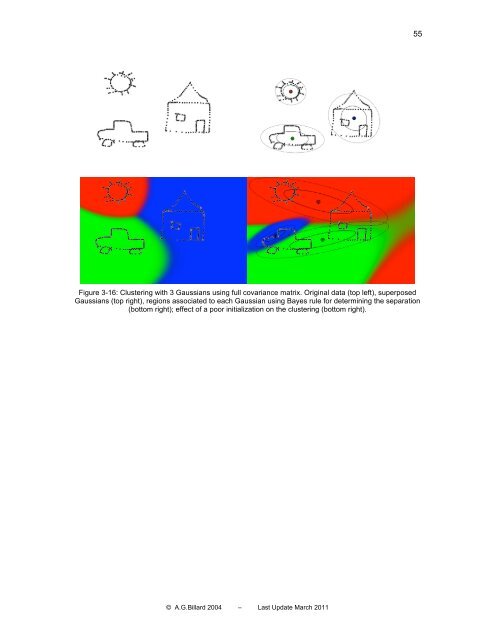
Page 53: 53 Theα are the so-called mixing c
Page 57 and 58: 57 When the transformation A is lin
Page 59 and 60: 59 C: X → Y ( ) C x K = arg max
Page 61 and 62: 61 Figure 3-18: Linear combination
Page 63 and 64: 63 Figure 3-19: Bayes classificatio
Page 65 and 66: 65 ⎛⎛ min ⎜⎜ w ⎝⎝ N i=
Page 67 and 68: 67 T ( yi − xi w) 2 M ⎛⎛ ⎞
Page 69 and 70: 69 Figure 4-2: Illustration of the
Page 71 and 72: 71 4.4.2 Multi-Gaussian Case It is
Page 73 and 74: 73 5 Kernel Methods These lecture n
Page 75 and 76: 75 The kernel k provides a metric o
Page 77 and 78: 77 M 1 T v = ∑ x ( x ) v M λ i j
Page 79 and 80: 79 1 M The solutions to the dual ei
Page 81 and 82: 81 5.4 Kernel CCA The linear versio
Page 83 and 84: 83 additional ridge parameter induc
Page 85 and 86: 85 Figure 5-3: TOP: Marginal (left)
Page 87 and 88: 87 statistical independence. We def
Page 89 and 90: 89 J j ( µ 1,...., µ K) = ∑∑
Page 91 and 92: 91 A simple pattern recognition alg
Page 93 and 94: 93 ( ) ( , ) f x = sign w x + b (5.
Page 95 and 96: 95 Figure 5-6: A binary classificat
Page 97 and 98: 97 where N is the number of support
Page 99 and 100: 99 5.8 Support Vector Regression In
Page 101 and 102: 101 The optimization problem given
Page 103 and 104: 103 Note that since we never have t
Page 105 and 106:
105 Figure 5-13: Effect of the kern
Page 107 and 108:
107 To better understand the effect
Page 109 and 110:
109 5.9 Gaussian Process Regression
Page 111 and 112:
111 One can then use the above expr
Page 113 and 114:
113 5.9.2 Equivalence of Gaussian P
Page 115 and 116:
115 5.9.3 Curse of dimensionality,
Page 117 and 118:
117 The weight w determines the slo
Page 119 and 120:
119 Figure 5-21: Example of success
Page 121 and 122:
121 • its performance tends to de
Page 123 and 124:
123 neurons. Furthermore, they lear
Page 125 and 126:
125 The sigmoid f x ( x) ( ) = tanh
Page 127 and 128:
127 6.3.2 Information Theory and th
Page 129 and 130:
129 ( R) ⎛⎛det ⎞⎞ I( x, y)
Page 131 and 132:
131 y= ∑ w x ) of Because of the
Page 133 and 134:
133 6.5 Willshaw net David Willshaw
Page 135 and 136:
135 6.6.1 Weights bounds One of the
Page 137 and 138:
137 Figure 6-11: The weight vector
Page 139 and 140:
139 6.6.4 Oja’s one Neuron Model
Page 141 and 142:
141 If y i and y are highly correla
Page 143 and 144:
143 Foldiak’s second model allows
Page 145 and 146:
145 ∂ ∂ J 1 = fy − 1 2 λ 1yf
Page 147 and 148:
147 6.8 The Self-Organizing Map (SO
Page 149 and 150:
149 6. Decrease the size of the nei
Page 151 and 152:
151 the resulting distribution is a
Page 153 and 154:
153 To simplify the description of
Page 155 and 156:
155 C µν −1 where ( ) is the µ
Page 157 and 158:
157 The continuous time Hopfield ne
Page 159 and 160:
159 ∂f If the slope is negative,
Page 161 and 162:
161 7.2 Hidden Markov Models Hidden
Page 163 and 164:
163 Figure 7-2: Schematic illustrat
Page 165 and 166:
165 these two quantities to compute
Page 167 and 168:
167 7.2.4 Decoding an HMM There are
Page 169 and 170:
169 7.2.5 Further Readings Rabiner,
Page 171 and 172:
171 7.3.1 Principle In reinforcemen
Page 173 and 174:
173 general, acting to maximize imm
Page 175 and 176:
175 of reinforcement learning makes
Page 177 and 178:
177 8 Genetic Algorithms We conclud
Page 179 and 180:
179 However, you must define geneti
Page 181 and 182:
181 Often the crossover operator an
Page 183 and 184:
183 ( A λI) x 0 − = (8.5) where
Page 185 and 186:
185 Joint probability: The joint pr
Page 187 and 188:
187 The two most classical distribu
Page 189 and 190:
189 9.2.7 Statistical Independence
Page 191 and 192:
191 1 1 1 1 h x ∫ a b a b 0 a a
Page 193 and 194:
193 9.4 Estimators 9.4.1 Gradient d
Page 195 and 196:
195 9.4.2.1 Maximum Likelihood Mach
Page 197 and 198:
197 10 References • Machine Learn
show all

MACHINE LEARNING TECHNIQUES - LASA

You also want an ePaper? Increase the reach of your titles

Delete template?

Save as template?