MACHINE LEARNING TECHNIQUES - LASA

165
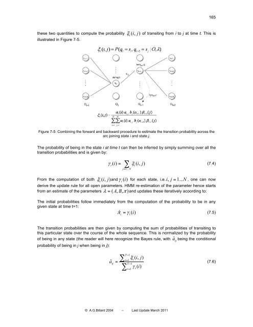
these two quantities to compute the probability (, i j)
illustrated in Figure 7-5.
ξ of transiting from i to j at time t. This is
t
Figure 7-5: Combining the forward and backward procedure to estimate the transition probability across the
arc joining state i and state j.
The probability of being in the state i at time t can then be inferred by simply summing over all the
transition probabilities and is given by:
γ () i = ∑ ξ (, i j)
(7.4)
t
j=
1... N
From the computation of both ξt
(, i j)
and γ
t
() i for each state, i.e. i, j = 1... N , one can now
derive the update rule for all open parameters. HMM re-estimation of the parameter hence starts
from an estimate of the parameters λ = ( AB , , π)
and updates these iteratively acoording to:
The initial probabilities follow immediately from the computation of the probability to be in any
given state at time t=1:
ˆ π = γ () i
(7.5)
i
1
t
The transition probabilities are then given by computing the sum of probabilities of transiting to
this particular state over the course of the whole sequence. This is normalized by the probability
of being in any state (the reader will here recognize the Bayes rule, with aˆij
being the conditional
probability of being in j when being in j):
aˆ
ij
T −1
ξ (, i j)
t=
1 t
T −1
= ∑ ∑ =
t 1
γ () i
t
(7.6)
© A.G.Billard 2004 – Last Update March 2011