Some Aspects of Hamilton-Jacobi Integrability and Separability
Some Aspects of Hamilton-Jacobi Integrability and Separability
Some Aspects of Hamilton-Jacobi Integrability and Separability

Create successful ePaper yourself
Turn your PDF publications into a flip-book with our unique Google optimized e-Paper software.
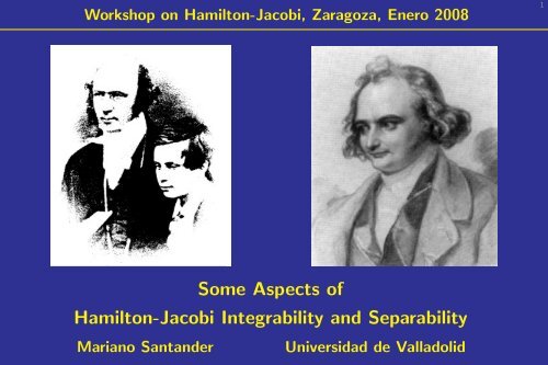
Workshop on <strong>Hamilton</strong>-<strong>Jacobi</strong>, Zaragoza, Enero 2008<br />
1<br />
<strong>Some</strong> <strong>Aspects</strong> <strong>of</strong><br />
<strong>Hamilton</strong>-<strong>Jacobi</strong> <strong>Integrability</strong> <strong>and</strong> <strong>Separability</strong><br />
Mariano Sant<strong>and</strong>er Universidad de Valladolid
Basics on the <strong>Hamilton</strong>-<strong>Jacobi</strong> equation<br />
2<br />
• History <strong>Hamilton</strong> attempt to formulate Mechanics as modelled after paraxial<br />
geometric Optics<br />
⋆ Optical axis as the time axis<br />
⋆ Optical Image plane as Space at an instant<br />
⋆ Simplectic structure behind (geometrical) optics appear as some<br />
important structure in Mechanics: the shadow <strong>of</strong> the canonical symplectic<br />
structure in Quantum Mechanics.<br />
• Fermat principle<br />
action<br />
as <strong>Hamilton</strong> principle: optical lenght as the <strong>Hamilton</strong>’s<br />
• Eikonal equation as the <strong>Hamilton</strong>-<strong>Jacobi</strong> equation.<br />
W.R. <strong>Hamilton</strong>, Theory <strong>of</strong> systems <strong>of</strong> rays, Transactions Royal Irish<br />
Academy, 15, 69-174 (1828)<br />
W.R. <strong>Hamilton</strong>, On the application to Dynamics <strong>of</strong> a general Mathematical<br />
Method previously applied to optics, British Association Report,<br />
Edinburgh, 513-518 (1835)
Basics on the <strong>Hamilton</strong>-<strong>Jacobi</strong> equation<br />
3<br />
• Visionary character <strong>of</strong> <strong>Hamilton</strong> contribution<br />
⋆ The ‘fundamental analogy’<br />
Geometric Optics : Ondulatory Optics<br />
::<br />
Classical Mechanics : Quantum Mechanics<br />
• <strong>Hamilton</strong>-<strong>Jacobi</strong> equation as the shadow <strong>of</strong> Schrödinger equation.<br />
• Classical mechanics as a double approximation from Quantum Mechanics<br />
<strong>and</strong> from Relativity: short wavelenght λ → 0 <strong>and</strong> paraxial approximation.<br />
⋆ <strong>Hamilton</strong>’s action is from a viewpoint the non-relativistic remnant <strong>of</strong><br />
the difference between proper <strong>and</strong> coordinate time S = mc 2 (τ − t)<br />
⋆ And from another one, <strong>Hamilton</strong>’s action registers the phase <strong>of</strong> the<br />
quantum amplitudes (Feynmann formulation, S = ¯hφ)
The History <strong>of</strong> <strong>Hamilton</strong>-<strong>Jacobi</strong> equation<br />
4<br />
• <strong>Hamilton</strong> contribution Mechanics as a consequence <strong>of</strong> a extremal principle.<br />
Action functional as the time integral <strong>of</strong> Lagrangian.<br />
⋆ Consider the ‘<strong>Hamilton</strong> principal function’ defined as the value <strong>of</strong><br />
the action along the actual trajectories S(x, t). Now <strong>Hamilton</strong> saw that<br />
this function is a solution <strong>of</strong> a partial differential equation, the mechanical<br />
analogue <strong>of</strong> the optics eikonal equation.<br />
1<br />
⋆ The equation is obtained as a translation <strong>of</strong><br />
2m p2 + V (x) = E under<br />
correspondence rules: p ↦→ ∇S, E ↦→ − ∂S<br />
∂t<br />
1<br />
2m (∇S)2 + V (x) = − ∂S<br />
∂t<br />
• <strong>Jacobi</strong> contribution He realized that also the converse was true; any solution<br />
<strong>of</strong> this equation can be used to solve the motion problem, by means <strong>of</strong> some<br />
canonical transformation.<br />
• Useful as an actual tool to solve specific problems? Indeed this is only<br />
useful in practice when it is possible to separate variables.
The Mathematics <strong>of</strong> <strong>Hamilton</strong>-<strong>Jacobi</strong> equation<br />
5<br />
• As a partial differential equation we note the essential appearance <strong>of</strong><br />
the Laplace operator ∇ 2<br />
⋆ This the the only second-order differential operator invariant (scalar)<br />
under the Euclidean isometry group<br />
• Extension to more general configuration spaces Natural stages: Zero<br />
curvature; Constant Curvature; General Riemannian space.<br />
⋆ Eventually, also Minkowskian configuration spaces<br />
• Is there some geometrical meaning <strong>of</strong> separability? Not an easy question;<br />
because separability depends on the coordinate system.<br />
• Now look to any classical book on Mechanics The odds are that they<br />
use either the harmonic oscillator or the Kepler problem as an illustration <strong>of</strong><br />
HJ.<br />
• Both systems are distinguished by the existence <strong>of</strong> an ‘abnormaly large’<br />
number <strong>of</strong> constants <strong>of</strong> motion. And in both the HJ equation turns out<br />
to be separable in several coordinate systems.
Constants <strong>of</strong> motion for the two ‘principal cases’<br />
6<br />
• Harmonic Oscillator<br />
(second order).<br />
Angular momentum (first order) <strong>and</strong> Fradkin tensor<br />
• Kepler-Coulomb problem Angular momentum (first order) <strong>and</strong> Laplace-<br />
Runge-Lenz vector (second order)<br />
• Fradkin conserved tensor <strong>and</strong> Runge-Lenz conserved vector appear<br />
precisely as linked to irreducible sets <strong>of</strong> constants <strong>of</strong> motion coming from the<br />
separability <strong>of</strong> <strong>Hamilton</strong>-<strong>Jacobi</strong> equation for the Harmonic oscillator <strong>and</strong> the<br />
Kepler-Coulomb potentials in several coordinate systems:<br />
⋆ Runge-Lenz vector is related to separability <strong>of</strong> the HJ equation for the<br />
Kepler potential in a full 1-d family <strong>of</strong> parabolic coordinates, with a focus<br />
at the origin<br />
A 1 = Jẏ − k cos φ, A 2 = −Jẋ − k sin φ, (1)<br />
⋆ Fradkin tensor related to separability <strong>of</strong> Harmonic oscillator potential in<br />
a full 1-d family <strong>of</strong> cartesian coordinates with any axes orientation<br />
F 11 = (ẋ) 2 + ω 2 0 x 2 , F 12 = F 21 = ẋẏ + ω 2 0 xy, F 22 = (ẏ) 2 + ω 2 0 y 2 . (2)
<strong>Integrability</strong> <strong>and</strong> separability <strong>of</strong> <strong>Hamilton</strong>-<strong>Jacobi</strong> equation in E 2<br />
7<br />
• Is there any relation between existence <strong>of</strong> constants <strong>of</strong> motion <strong>and</strong><br />
separability <strong>of</strong> the HJ equation?<br />
• Classical <strong>Integrability</strong> Existence <strong>of</strong> constants <strong>of</strong> motion. For n = 2 a single<br />
constant ensures integrability, no restriction due to involution condition.<br />
• Noether constant related with invariance under some one-parameter group <strong>of</strong><br />
symmetries (a subgroup <strong>of</strong> the Euclidean group). First order in the velocities.<br />
⋆ These symmetries are clearly related to the separability <strong>of</strong> the HJ<br />
equation for the Harmonic oscillator <strong>and</strong> for the Kepler potential in polar<br />
coordinates.<br />
⋆ Are there other Noether constants responsible <strong>of</strong> the separability <strong>of</strong><br />
HJ equation for harmonic oscillator in cartesian coordinates or <strong>of</strong> the HJ<br />
for Kepler in parabolic coordinates? No
<strong>Integrability</strong> <strong>and</strong> separability <strong>of</strong> <strong>Hamilton</strong>-<strong>Jacobi</strong> equation in E 2 II<br />
8<br />
• Are there other constants (not <strong>of</strong> Noether type) responsible <strong>of</strong> / linked<br />
to the separability <strong>of</strong> HJ equation for harmonic oscillator in cartesian<br />
coordinates or <strong>of</strong> the HJ for Kepler in parabolic coordinates? Yes<br />
• Next type <strong>of</strong> constants <strong>of</strong> motion are required to be quadratic in the<br />
velocities (similar to the energy). Precisely these constants are related to<br />
separability <strong>of</strong> <strong>Hamilton</strong>-<strong>Jacobi</strong> equation.<br />
• <strong>Separability</strong> <strong>of</strong> <strong>Hamilton</strong> <strong>Jacobi</strong> equation is possible only in some coordinate<br />
systems, determined independently <strong>of</strong> the potential (i.e., for the<br />
free <strong>Hamilton</strong>-<strong>Jacobi</strong> equation) <strong>and</strong> once a such system is fixed, it requires<br />
additionally the potential to have some special form, called Stäckel or<br />
separable form, in these coordinates.<br />
• When these conditions are met there always exists a constant <strong>of</strong> motion<br />
which is quadratic in the velocities. Exceptionally, this constant may come<br />
as the square <strong>of</strong> a constant which is first order in the velocities.
Dynamics on a constant curvature 2d space<br />
9<br />
• Motion <strong>of</strong> a particle in the configuration space under a natural mechanical<br />
type Lagrangian<br />
L = 1 2 g µν(q 1 , q 2 )v q µv q ν − V(q 1 , q 2 ).<br />
⋆ <strong>Hamilton</strong>ian<br />
H = 1 2 gµν (q 1 , q 2 )p µ p ν + V(q 1 , q 2 ).<br />
⋆ Configuration space: either the Euclidean plane, or a space with<br />
constant curvature, or a Riemannian space with a general metric<br />
(or even a Lorentzian configuration space, with a non-definite metric)<br />
• Restrict to the constant curvature case. The leading idea is to see how<br />
properties change when the configuration space acquires non-zero curvature.<br />
• <strong>Hamilton</strong>-<strong>Jacobi</strong> equation now involves the Laplace-Beltrami operator<br />
<strong>of</strong> the metric
Systems allowing linear constants <strong>of</strong> motion, n = 2<br />
10<br />
• Which is the most general system allowing constants <strong>of</strong> motion linear<br />
in the velocities?<br />
• The system must be invariant under a one-parameter subgroup <strong>of</strong><br />
(Euclidean, spherical, hyperbolic) isometries<br />
⋆ Noether momenta Denote P 1 , P 2 , J 12 , the Noether momenta associated<br />
to translations along two orthogonal lines l 1 , l 2 <strong>and</strong> rotations around O =<br />
l 1 ∩ l 2 .<br />
⋆ The most general constant <strong>of</strong> motion linear in the velocities is<br />
I = a 12 J 12 + +a 1 P 1 + a 2 P 2<br />
⋆ Free part <strong>of</strong> <strong>Hamilton</strong>-<strong>Jacobi</strong> equation (Laplace-Beltrami operator)<br />
is automatically invariant under the subgroup generated by I No<br />
restriction here.<br />
⋆ Potential invariance condition singles out potentials rotationally invariant<br />
(around a center, central potentials) <strong>and</strong> translationally invariant<br />
(‘one-dimensional’ potentials). This works exactly alike in the non-flat case.
Linear constants <strong>of</strong> motion. Direct approach<br />
11<br />
• Are there constants <strong>of</strong> motion which are linear in the velocities?<br />
• Possible constants are <strong>of</strong> the form I K = K µ (q 1 , q 2 ) v q µ. This is actually<br />
a constant <strong>of</strong> motion provided K µ (q 1 , q 2 ) satisfies some equations involving<br />
the data g µν (q 1 , q 2 ), V(q 1 , q 2 ).<br />
⋆ These equations split in two sets. The first is independent <strong>of</strong> the potential,<br />
<strong>and</strong> restricts how the vector field K µ (q 1 , q 2 ) can depend on coordinates.<br />
⋆ There is some geometric meaning in the equations in the first set?<br />
K µ (q 1 , q 2 ) is a Killing vector field for the metric <strong>of</strong> the space.<br />
I K = K µ (q 1 , q 2 ) v q µv q ν = a 0 J + a 1 P 1 + a 2 P 2<br />
• Once a Killing vector field has been chosen the remaining equation to be<br />
satisfied by the potential is the usual invariance requirement. Geometrically,<br />
the potential must be invariant under the isometries generated by the Killing<br />
vector field.
Linear constants <strong>of</strong> motion. Killing vector interpretation<br />
12<br />
• Free motion allow for three linearly independent constants <strong>of</strong> motion<br />
linear in the velocities. Suitable change <strong>of</strong> the basic l 1 , l 2 , O reduces any<br />
I K = a 0 J + a 1 P 1 + a 2 P 2 to either P 1 <strong>and</strong> J .<br />
⋆ Associated coordinate systems Rectifying coordinates for P 1 <strong>and</strong> J . In<br />
the euclidean plane these are respectively cartesian coordinates <strong>and</strong> polar<br />
coordinates. On the sphere <strong>and</strong> the hyperbolic plane these are its analogous<br />
(geodesic parallel <strong>and</strong> geodesic polar coordinates)<br />
⋆ <strong>Some</strong> authors call these coordinates ‘group coordinates’<br />
⋆ Non-free systems with a given potential will keep a such linear<br />
constant I = a 0 J + a 1 P 1 + a 2 P 2 as long as the potential is invariant<br />
under the one-parameter subgroup generated by I.<br />
⋆ In terms <strong>of</strong> the associated group coordinates, the condition can be<br />
formulated geometrically as ‘the potential does depend only on a single<br />
coordinate’. But beware!<br />
• Close connection between Killing vectors <strong>and</strong> constant <strong>of</strong> motion linear in<br />
the velocities.
Constants <strong>of</strong> motion quadratic in the velocities. Direct approach<br />
13<br />
• Are there constants <strong>of</strong> motion I which are quadratic in the velocities?<br />
⋆ Possible constants I K = K µν (q 1 , q 2 ) v q µv q ν + W(q 1 , q 2 ).<br />
• The requirement for I K to be a constant <strong>of</strong> motion translates into<br />
some conditions on K µν <strong>and</strong> W These conditions split in two subsets.<br />
• First subset, independent <strong>of</strong> the potential V Thus this might be expected<br />
to depend only on some property <strong>of</strong> the free <strong>Hamilton</strong>-<strong>Jacobi</strong> equation.<br />
Which property?<br />
• Not obvious at all These equations appear in several classical papers <strong>and</strong><br />
books.<br />
⋆ Geometric interpretation: the tensor K µν should be a Killing tensor for<br />
the metric g µν .<br />
⋆ After all, a rather natural extension to the first order case<br />
⋆ Most general solution to these equations :<br />
K µν (q 1 , q 2 ) v q µv q ν = a 0 J 2 + a 1 P 2 1 + a 2 P 2 2 + 2a 01 J P 1 + 2a 02 J P 2 + 2a 12 P 1 P 2 (3)
Constants <strong>of</strong> motion quadratic in the velocities. Direct approach II<br />
14<br />
• Once a Killing tensor K µν has been fixed , the second subset <strong>of</strong> conditions<br />
(which would determine W) depend actually on the potential V. These are<br />
a system <strong>of</strong> partial differential equations for W; its compatibility equation is<br />
a single differential equation for the potential V.<br />
⋆ Essentially this equation dates (in the euclidean case, in general<br />
coordinates) from Levi-Civita<br />
• Geometric meaning Not direct, but somehow a kind <strong>of</strong> ‘second order invariance’
Killing tensors <strong>and</strong> confocal coordinate systems<br />
15<br />
• Connection between Killing vectors <strong>and</strong> group coordinates Each Killing<br />
vector determines a coordinate web in the space (associated to the group<br />
coordinates; e.g. for euclidean plane these are either cartesian or polar)<br />
⋆ Potentials allowing for a Killing vector as a constant <strong>of</strong> motion have<br />
a special dependence on these coordinates<br />
• Each Killing tensor also determines a coordinate web in the configuration<br />
space. But coordinates are not ‘group coordinates’<br />
• Potentials allowing a I K -type quadratic constant <strong>of</strong> motion are precisely<br />
those which are separable in the coordinate system associated to this<br />
web.<br />
⋆ W can be determined also starting from the separable form <strong>of</strong> V.<br />
• Coordinates are secondary, the web is the important thing<br />
• Main problem: find the coordinate webs associated to the more general<br />
Killing tensor
Systems allowing quadratic constants <strong>of</strong> motion: elliptic coordinates<br />
16<br />
• Most general coordinates associated to Killing tensors? These are<br />
precisely coordinate systems allowing the (free) <strong>Hamilton</strong>-<strong>Jacobi</strong> equation to<br />
be separated.<br />
• In the euclidean case<br />
⋆ For coordinates: Liouville Elliptic coordinates (Euler) <strong>and</strong> their three limiting<br />
cases (polar coordinates, parabolic coordinates, cartesian coordinates).<br />
Non-group coordinates versus group coordinates.<br />
⋆ For the potential: Stäckel, Eisenhart The potential must be separable<br />
in a coordinate system in the previous list.
Elliptic coordinates in E 2<br />
17<br />
• For instance, elliptic coordinates with foci F 1 , F 2 symmetrically placed<br />
relative to the origin, with separation 2f<br />
Elliptic coordinates ( r 1+r 2<br />
, r 1−r 2<br />
).<br />
2 2<br />
Separable potentials: V = 1 ) + B( r 1+r 2<br />
) }<br />
2 2<br />
Constant <strong>of</strong> motion:<br />
(J 2 − f 2 P 2 1 )+ 1<br />
r 1 r 2<br />
{<br />
A(<br />
r 1 +r 2<br />
{(<br />
(<br />
r 1 +r 2<br />
) 2 − f 2) B( r 1−r 2<br />
) − ( f 2 − ( r 1−r 2<br />
) 2) A( r 1+r 2<br />
) }<br />
2 2 2 2<br />
r 1 r 2<br />
• The non-generic limits can be dealt with accordingly<br />
⋆ Polar Both foci coincide<br />
⋆ Parabolic One focus go to infinity<br />
⋆ Cartesian Both foci go to infinity
Killing tensors <strong>and</strong> elliptic coordinates on curved spaces<br />
18<br />
• Main problem: In a space with any constant curvature, find the coordinate<br />
webs associated to the more general Killing tensor<br />
• Generic Confocal webs Curves with r 1 ±r 2 , ˜r 1 ± ˜r 2 , r 1 ± ˜r 2 equal to constant,<br />
with r 1 , r 2 , . . . determined as:<br />
⋆ A pair <strong>of</strong> focal points, r 1 , r 2 denoting the intrinsic distances to these foci<br />
(Elliptic ).<br />
⋆ A pair <strong>of</strong> focal lines, ˜r 1 , ˜r 2 denoting the intrinsic distances to these focal<br />
lines (UltraElliptic ).<br />
⋆ A pair made <strong>of</strong> a focal point <strong>and</strong> a focal line, with r 1 , ˜r 2 denoting the<br />
intrinsic distances to these focal elements (Parabolic ).<br />
• Particular or Limiting Confocal webs where focal elements either coincide<br />
or go to infinity if possible at all.<br />
⋆ The number <strong>of</strong> cases depend on whether there is an actual infinity (as<br />
in H 2 ) or not (as in S 2 )
The elliptic coordinate system in the curved case<br />
19<br />
• Space with constant curvature κ<br />
• Consider the web associated to elliptic coordinates determined by two<br />
foci F 1 , F 2 with separation 2f Basic generic system in all cases.<br />
⋆ Elliptic coordinates ( r 1+r 2<br />
, r 1−r 2<br />
).<br />
2 2 {<br />
1<br />
⋆ Separable potentials: V =<br />
S κ1 (r 1 ) S κ1 (r 2 ) A(<br />
r 1 +r 2<br />
) + B( r 1+r 2<br />
) }<br />
2 2<br />
⋆ Constant ( <strong>of</strong> motion: )<br />
C<br />
2<br />
κ1<br />
(f)J 2 − S 2 κ 1<br />
(f)P1<br />
2 +<br />
1 {(<br />
S<br />
2<br />
S κ1 (r 1 ) S κ1 (r 2 )<br />
κ1<br />
( r 1+r 2<br />
) − S 2 2 κ 1<br />
(f) ) B( r 1−r 2<br />
) − ( S 2 2 κ 1<br />
(f) − S 2 κ 1<br />
( r 1−r 2<br />
) ) A( r 1+r 2<br />
) }<br />
2 2<br />
⋆ Labeled Trigonometric functions: ‘cosine’ C κ (x) <strong>and</strong> ‘sine’ S κ (x), ‘label’<br />
κ:<br />
⎧<br />
⎪⎨ cos √ ⎧<br />
κ x<br />
√1<br />
⎪⎨ κ<br />
sin √ κ x κ > 0<br />
C κ (x) := 1<br />
⎪⎩<br />
cosh √ S κ (x) := x κ = 0<br />
−κ x<br />
⎪⎩ √1<br />
−κ<br />
sinh √ . (4)<br />
−κ x κ < 0
The classification <strong>of</strong> (real) confocal coordinate systems in H 2<br />
20<br />
• Depicted in the Poincaré conformal Half plane model, doubled for<br />
graphic convenience<br />
⋆ Two copies <strong>of</strong> the hyperbolic plane glued by the circle at infinity
Non-obvious integrable systems in spaces <strong>of</strong> constant curvature<br />
21<br />
• Basic classification in types <strong>of</strong> constants: two constants are <strong>of</strong> the<br />
same type if their Killing tensor part is the same<br />
• But constants <strong>of</strong> motion are linear If I 1 , I 2 are constants <strong>of</strong> motion, so it<br />
is αI 1 + βI 2 .<br />
• In particular this means that if a particular system admits two constants<br />
<strong>of</strong> motion <strong>of</strong> quadratic type, with Killing tensors W 1 , W 2 , then it the<br />
HJ equation is separable in two different coordinate systems.<br />
• Now the system admits a one-parameter infinite family <strong>of</strong> Killing tensors<br />
αW 1 + βW 2 . And in turn this means that the HJ eqution is separable<br />
not only in two coordinate systems, but in any member <strong>of</strong> a infinite<br />
family (depending essentially <strong>of</strong> a single parameter β/α).<br />
• This elementary observation can be used to conclude, whitout any<br />
computation, that some non-trivial systems are integrable <strong>and</strong> HJ separable.
An example <strong>of</strong> integrable system in spaces <strong>of</strong> constant curvature<br />
22<br />
• Consider the problem with two Kepler-Coulomb centers Since Euler<br />
this system on the Euclidean plane has been known to be integrable.<br />
• Is this system integrable on a constant curvature space?<br />
• The curved Kepler problem has constants <strong>of</strong> types J 2 , associated to polar<br />
(double focus at the origin) <strong>and</strong> J P 2 , associated to parabolic coordinates<br />
(a focus at the origin).<br />
⋆ As constants are linear, it follows that Kepler has also a constant <strong>of</strong><br />
type J (J + λP 2 ). This is associated to a system <strong>of</strong> elliptic coordinates,<br />
with a focus at origin <strong>and</strong> the other on the axis <strong>of</strong> the initial parabolic<br />
system. All such interpolating elliptic systems appear by tuning λ.<br />
• Thus Kepler has constants <strong>of</strong> the type associated to all elliptic coordinates<br />
with a focus at the origin <strong>and</strong> is therefore separable in all these<br />
coordinate systems.<br />
• The problem with two Kepler-Coulomb centers is therefore separable,<br />
for any constant curvature, in the elliptic coordinate system with the two<br />
focus at the two centers.
<strong>Some</strong> recent references<br />
23<br />
⋆ J.F. Cariñena, M.F. Rañada, M.S., Superintegrability in curved spaces,<br />
orbits <strong>and</strong> momentum hodographs: revisiting a classical result by<br />
<strong>Hamilton</strong>, (J. Phys. A)<br />
⋆ J.F. Cariñena, M.F. Rañada, M.S., The harmonic oscillator on Riemannian<br />
<strong>and</strong> Lorentzian configuration spaces <strong>of</strong> constant curvature, To<br />
appear in J. Math. Phys, arXiv: 0709.2572 [math-ph]