A Generalized MVDR Spectrum - ResearchGate

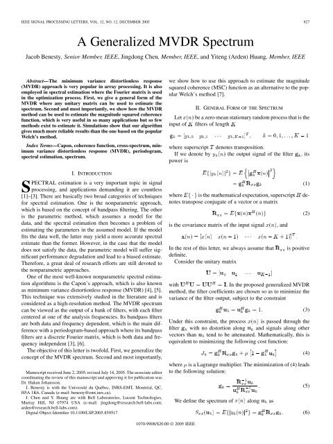
IEEE SIGNAL PROCESSING LETTERS, VOL. 12, NO. 12, DECEMBER 2005 827
A Generalized MVDR Spectrum
Jacob Benesty, Senior Member, IEEE, Jingdong Chen, Member, IEEE, and Yiteng (Arden) Huang, Member, IEEE
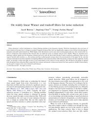
Abstract—The minimum variance distortionless response
(MVDR) approach is very popular in array processing. It is also
employed in spectral estimation where the Fourier matrix is used
in the optimization process. First, we give a general form of the
MVDR where any unitary matrix can be used to estimate the
spectrum. Second and most importantly, we show how the MVDR
method can be used to estimate the magnitude squared coherence
function, which is very useful in so many applications but so few
methods exist to estimate it. Simulations show that our algorithm
gives much more reliable results than the one based on the popular
Welch’s method.
Index Terms—Capon, coherence function, cross-spectrum, minimum
variance distortionless response (MVDR), periodogram,
spectral estimation, spectrum.
I. INTRODUCTION
SPECTRAL estimation is a very important topic in signal
processing, and applications demanding it are countless
[1]–[3]. There are basically two broad categories of techniques
for spectral estimation. One is the nonparametric approach,
which is based on the concept of bandpass filtering. The other
is the parametric method, which assumes a model for the
data, and the spectral estimation then becomes a problem of
estimating the parameters in the assumed model. If the model
fits the data well, the latter may yield a more accurate spectral
estimate than the former. However, in the case that the model
does not satisfy the data, the parametric model will suffer significant
performance degradation and lead to a biased estimate.
Therefore, a great deal of research efforts are still devoted to
the nonparametric approaches.
One of the most well-known nonparametric spectral estimation
algorithms is the Capon’s approach, which is also known
as minimum variance distortionless response (MVDR) [4], [5].
This technique was extensively studied in the literature and is
considered as a high-resolution method. The MVDR spectrum
can be viewed as the output of a bank of filters, with each filter
centered at one of the analysis frequencies. Its bandpass filters
are both data and frequency dependent, which is the main difference
with a periodogram-based approach where its bandpass
filters are a discrete Fourier matrix, which is both data and frequency
independent [3], [6].
The objective of this letter is twofold. First, we generalize the
concept of the MVDR spectrum. Second and most importantly,
Manuscript received June 2, 2005; revised July 14, 2005. The associate editor
coordinating the review of this manuscript and approving it for publication was
Dr. Hakan Johansson.
J. Benesty is with the Université du Québec, INRS-EMT, Montréal, QC,
H5A 1K6, Canada (e-mail: benesty@emt.inrs.ca).
J. Chen and Y. Huang are with Bell Laboratories, Lucent Technologies,
Murray Hill, NJ 07974 USA (e-mail: jingdong@research.bell-labs.com;
arden@research.bell-labs.com).
Digital Object Identifier 10.1109/LSP.2005.859517
we show how to use this approach to estimate the magnitude
squared coherence (MSC) function as an alternative to the popular
Welch’s method [7].
Let
input of
II. GENERAL FORM OF THE SPECTRUM
be a zero-mean stationary random process that is the
filters of length
where superscript denotes transposition.
If we denote by the output signal of the filter , its
power is
where is the mathematical expectation, superscript denotes
transpose conjugate of a vector or a matrix
is the covariance matrix of the input signal
In the rest of this letter, we always assume that
definite.
Consider the unitary matrix
, and
(1)
(2)
is positive
with
. In the proposed generalized MVDR
method, the filter coefficients are chosen so as to minimize the
variance of the filter output, subject to the constraint
Under this constraint, the process is passed through the
filter with no distortion along and signals along other
vectors than tend to be attenuated. Mathematically, this is
equivalent to minimizing the following cost function:
where is a Lagrange multiplier. The minimization of (4) leads
to the following solution:
We define the spectrum of along as
(3)
(4)
(5)
(6)
1070-9908/$20.00 © 2005 IEEE

828 IEEE SIGNAL PROCESSING LETTERS, VOL. 12, NO. 12, DECEMBER 2005
Therefore, plugging (5) into (6), we find that
(7)
The first obvious choice for the unitary matrix
Fourier matrix
is the
Expression (7) is a general definition of the spectrum of the
signal , which depends on the unitary matrix . Replacing
the previous equation in (5), we get
where
Taking into account all vectors
the general form
where
(8)
, (8) has
(9)
and . Of course, is a
unitary matrix. With this choice, we obtain the classical Capon’s
method.
Now suppose . In this case, a Toeplitz matrix is
asymptotically equivalent to a circulant matrix if its elements
are absolutely summable [8], which is usually the case in most
applications. Hence, we can decompose as
(12)
and
diag
is a diagonal matrix.
Property 1: We have
(10)
Proof: This form follows immediately from (9).
Property 1 shows that there are an infinite number of ways
to decompose matrix , depending on how we choose the
unitary matrix . Each one of these decompositions gives a
representation of the square of the spectrum of the signal
in the subspace .
Property 2: We have
Proof: Indeed
tr
tr tr (11)
tr
Property 2 expresses the energy conservation. So no matter
what we take for the unitary matrix , the sum of all values of
the inverse spectrum is always the same.
A. Particular Cases
In this subsection, we propose to briefly discuss three important
particular cases of the general form of the MVDR spectrum.
tr
tr
so that . As a result, for a stationary signal and asymptotically,
Capon’s approach is equivalent to the periodogram. The
difference between the MVDR and periodogram approaches can
also be viewed as the difference between the eigenvalue decompositions
of circulant and Toeplitz matrices. While for a circulant
matrix, its corresponding unitary matrix is data independent,
it is not for a Toeplitz matrix.
The second natural choice for is the matrix containing the
eigenvectors of the correlation matrix . Indeed, it is well
known that can be diagonalized as follows [9]:
(13)
where is a unitary matrix containing the eigenvectors , and
is a diagonal matrix containing the corresponding eigenvalues
. Thus, taking ,wefind that and
(14)
In many applications, the process signal is real, and it
may be more convenient to select an orthogonal matrix instead
of a unitary one. So our third and final particular case is the
discrete cosine transform
where the rest is shown in the equation at the bottom of the
page, with and for .We
can verify that
. So with this orthogonal
transform, the spectrum is
diag (15)

BENESTY et al.: GENERALIZED MVDR SPECTRUM 829
III. APPLICATION TO THE CROSS-SPECTRUM
AND MSC FUNCTION
In this section, we show how to use the generalized MVDR
approach for the estimation of the cross-spectrum and the MSC
function.
A. General Form of the Cross-Spectrum
We assume here that we have two zero-mean stationary
random signals and with respective spectra
and . As explained in Section II, we can
design two filters
For (23) to have the true sense of the cross-spectrum definition,
the matrix should be complex (and unitary).
Property 3: We have
tr
(24)
Proof: This is easy to see from (23).
Property 3 is similar to property 2 and shows another form of
energy conservation.
to find the spectra of and along
where
(16)
(17)
B. General Form of the MSC Function
We define the MSC function between two signals and
as
(25)
From (23), we deduce the magnitude squared cross-spectrum
(26)
is the covariance matrix of the signal
and
(18)
Using expressions (17) and (26) in (25), the MSC becomes
(27)
Property 4: We have
Let and be the respective outputs of the filters
and .Wedefine the cross-spectrum between and
along as
(19)
(28)
Proof: Since matrices and are assumed to
be positive definite, it is clear that
. To prove that
, we need to rewrite the MSC function. Define
the vectors
where the superscript
Similarly
is the complex conjugate operator.
and the normalized cross-correlation matrix
(29)
(30)
(20)
Using the previous definitions in (27), the MSC is now
Now if we develop (19), we get
where
(21)
(22)
is the cross-correlation matrix between and . Replacing
(16) in (21), we obtain the cross-spectrum
(23)
Consider the Hermitian positive semidefinite matrix
and the vectors
(31)
(32)
(33)
(34)

830 IEEE SIGNAL PROCESSING LETTERS, VOL. 12, NO. 12, DECEMBER 2005
We can easily check that
(35)
(36)
Inserting these expressions in the Cauchy–Schwartz inequality
(37)
we see that .
Property 4 was, of course, expected in order that the definition
(27) of the MSC could have a sense.
C. Simulation Example
In this subsection, we compare the MSC function estimated
with our approach and with the MATLAB function “cohere”
that uses the Welch’s averaged periodogram method [7]. We
consider the illustrative example of two signals and
that do not have that much in common, except for two sinusoids
at frequencies and
(38)
(39)
where and are two independent zero-mean (real)
white Gaussian random processes with unit variance. The
phases and in the signal are random. In this
example, the theoretical coherence should be equal to at
the two frequencies and and at the others. Here we
chose and . For both algorithms, we
took 1024 samples and a window of length . As for
the choice of the unitary matrix in our approach, we took the
Fourier matrix. Fig. 1(a) and (b) give the MSC estimated with
MATLAB and our method, respectively. Clearly, the estimation
of the coherence function with our algorithm is much closer to
its theoretical values.
IV. CONCLUSION
The MVDR principle is very popular in array processing
and spectral estimation. In this letter, we have shown that this
concept can be generalized to unitary matrices other than the
Fig. 1.
Estimation of the MSC function. (a) MATLAB function “cohere.” (b)
Proposed algorithm with U = F. Conditions of simulations: K =100and a
number of samples of 1024.
Fourier transform for spectrum evaluation. Most importantly,
we have given an alternative to the popular Welch’s method for
the estimation of the MSC function. Simulations show that the
new method works much better.
REFERENCES
[1] S. L. Marple, Jr., Digital Spectral Analysis with Applications. Englewood
Cliffs, NJ: Prentice-Hall, 1987.
[2] S. M. Kay, Modern Spectral Estimation: Theory and Application. Englewood
Cliffs, NJ: Prentice-Hall, 1988.
[3] P. Stoica and R. L. Moses, Introduction to Spectral Analysis. Upper
Saddle River, NJ: Prentice-Hall, 1997.
[4] J. Capon, “High resolution frequency-wavenumber spectrum analysis,”
Proc. IEEE, vol. 57, no. 8, pp. 1408–1418, Aug. 1969.
[5] R. T. Lacoss, “Data adaptive spectral analysis methods,” Geophys., vol.
36, pp. 661–675, Aug. 1971.
[6] P. Stoica, A. Jakobsson, and J. Li, “Matched-filter bank interpretation
of some spectral estimators,” Signal Process., vol. 66, pp. 45–59, Apr.
1998.
[7] P. D. Welch, “The use of fast Fourier transform for the estimation of
power spectra: A method based on time averaging over short, modified
periodograms,” IEEE Trans. Audio Electroacoust., vol. AU-15, no. 2,
pp. 70–73, Jun. 1967.
[8] R. M. Gray, “Toeplitz and Circulant Matrices: A Review,” Stanford
Univ., Stanford, CA, Int. Rep., 2002.
[9] S. Haykin, Adaptive Filter Theory, 4th ed. Englewood Cliffs, NJ: Prentice-Hall,
2002.