Weibull Analysis. - Statistics
Weibull Analysis. - Statistics
Weibull Analysis. - Statistics

Create successful ePaper yourself
Turn your PDF publications into a flip-book with our unique Google optimized e-Paper software.
STAT 498 B<br />
Industrial <strong>Statistics</strong><br />
<strong>Weibull</strong> <strong>Analysis</strong><br />
Fritz Scholz<br />
Spring Quarter 2008
The <strong>Weibull</strong> Distribution<br />
The 2-parameter <strong>Weibull</strong> distribution function is defined as<br />
[ ( ] x β<br />
F α,β (x) = 1 − exp −<br />
for x ≥ 0 and F<br />
α)<br />
α,β (x) = 0 for x < 0.<br />
Write X ∼ W (α,β) when X has this distribution function, i.e., P(X ≤ x) = F α,β (x).<br />
α > 0 and β > 0 are referred to as scale and shape parameter, respectively.<br />
The <strong>Weibull</strong> density has the following form<br />
f α,β (x) = F ′ α,β (x) = d dx F α,β (x) = β α<br />
( [ x β−1 ( ] x β<br />
exp −<br />
α)<br />
α)<br />
.<br />
For β = 1 the <strong>Weibull</strong> distribution = the exponential distribution with mean α.<br />
In general, α represents the .632-quantile of the <strong>Weibull</strong> distribution regardless of<br />
the value of β since F α,β (α) = 1 − exp(−1) ≈ .632 for all β > 0.<br />
1
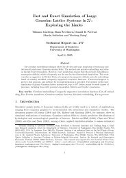
<strong>Weibull</strong> densities<br />
63.2%<br />
36.8%<br />
β 1 = 0.5<br />
β 2 = 1<br />
β 3 = 1.5<br />
β 4 = 2<br />
β 5 = 3.6<br />
β 6 = 7<br />
α = 10000<br />
α<br />
Note that the <strong>Weibull</strong> distribution spread around α ↘ as β ↗.<br />
The reason becomes clearer later when we discuss the log-transform Y = log(X).<br />
2
Moments and Quantiles<br />
The m th moment of the <strong>Weibull</strong> distribution is<br />
E(X m ) = α m Γ(1 + m/β)<br />
and thus the mean and variance are given by<br />
[<br />
µ = E(X) = αΓ(1 + 1/β) and σ 2 = α 2 Γ(1 + 2/β) − {Γ(1 + 1/β)} 2] .<br />
Its p-quantile, defined by P(X ≤ x p ) = p, is<br />
x p = α(−log(1 − p)) 1/β .<br />
For p = 1 − exp(−1) ≈ .632 (i.e., −log(1 − p) = 1) we have x p = α for all β > 0<br />
For that reason one also calls α the characteristic life of the <strong>Weibull</strong> distribution.<br />
The term life comes from the common use of the <strong>Weibull</strong> distribution in modeling<br />
lifetime data. More on this later.<br />
3
Minimum Closure Property<br />
If X 1 ,...,X n are independent with X i ∼ W (α i ,β), i = 1,...,n, then<br />
P(min(X 1 ,...,X n ) > t) = P(X 1 > t,...,X n > t) =<br />
=<br />
i.e., min(X 1 ,...,X n ) ∼ W (α ⋆ ,β).<br />
[<br />
n<br />
( ) ]<br />
t<br />
β<br />
∏ exp −<br />
i=1<br />
α i<br />
[ ( t<br />
) ] β<br />
= exp −<br />
α ⋆<br />
n<br />
∏<br />
i=1<br />
P(X i > t)<br />
⎡<br />
= exp⎣−t β ∑<br />
n<br />
with α ⋆ =<br />
⎛<br />
1<br />
i=1 α β i<br />
⎝ n ∑<br />
i=1<br />
1<br />
α β i<br />
⎤<br />
⎦<br />
⎞<br />
⎠<br />
−1/β<br />
,<br />
Similar to the closure property for the normal distribution under summation, i.e.,<br />
if X 1 ,...,X n are independent with X i ∼ N (µ i ,σ 2 i ) then<br />
)<br />
(<br />
n<br />
n∑<br />
∑ X i ∼ N<br />
i=1 i=1<br />
µ i ,<br />
n<br />
∑<br />
i=1<br />
σ 2 i<br />
.<br />
4
Limit Theorems<br />
This summation closure property is essential in proving the central limit theorem:<br />
Sums of independent random variables (not necessarily normally distributed) have<br />
an approximate normal distribution, subject to some mild conditions concerning the<br />
distribution of such random variables.<br />
There is a similar result from Extreme Value Theory that says:<br />
The minimum of independent, identically distributed random variables<br />
(not necessarily <strong>Weibull</strong> distributed) has an approximate <strong>Weibull</strong> distribution,<br />
subject to some mild conditions concerning the distribution of such random<br />
variables.<br />
This is also referred to as the weakest link motivation for the <strong>Weibull</strong> distribution.<br />
5
Weakest Link Motivation for <strong>Weibull</strong> Modeling<br />
The <strong>Weibull</strong> distribution is appropriate when trying to characterize the random<br />
strength of materials or the random lifetime of some system.<br />
A piece of material can be viewed as a concatenation of many smaller material<br />
cells, each of which has its random breaking strength X i when subjected to stress.<br />
Thus the strength of the concatenated total piece is the strength of its weakest link,<br />
namely min(X 1 ,...,X n ), i.e., approximately <strong>Weibull</strong>.<br />
Similarly, a system can be viewed as a collection of many parts or subsystems,<br />
each of which has a random lifetime X i .<br />
If the system is defined to be in a failed state whenever any one of its parts or<br />
subsystems fails =⇒ system lifetime is min(X 1 ,...,X n ), i.e., approximately <strong>Weibull</strong>.<br />
6
Waloddi <strong>Weibull</strong><br />
8
<strong>Weibull</strong> Distribution Popularity<br />
The <strong>Weibull</strong> distribution is very popular among engineers. One reason for this is<br />
that the <strong>Weibull</strong> cdf has a closed form which is not the case for the normal cdf Φ(x).<br />
Another reason for the popularity of the <strong>Weibull</strong> distribution among engineers may<br />
be that <strong>Weibull</strong>’s most famous paper, originally submitted to a statistics journal<br />
and rejected, was eventually published in an engineering journal:<br />
Waloddi <strong>Weibull</strong> (1951) “A statistical distribution function of wide applicability.”<br />
Journal of Applied Mechanics, 18, 293-297.<br />
9
Göran W. <strong>Weibull</strong> (1981):<br />
“... he tried to publish an article in a well-known British journal. At this time, the<br />
distribution function proposed by Gauss was dominating and was distinguishingly<br />
called the normal distribution. By some statisticians it was even believed to be the<br />
only possible one. The article was refused with the comment that it was interesting<br />
but of no practical importance. That was just the same article as the highly cited<br />
one published in 1951.”<br />
http://www.garfield.library.upenn.edu/classics1981/A1981LD32400001.pdf)<br />
10
Sam Saunders (1975):<br />
‘Professor Wallodi (sic) <strong>Weibull</strong> recounted to me that the now famous paper of<br />
his “A Statistical Distribution of Wide Applicability”, in which was first advocated<br />
the “<strong>Weibull</strong>” distribution with its failure rate a power of time, was rejected by the<br />
Journal of the American Statistical Association as being of no interrest. Thus one<br />
of the most influential papers in statistics of that decade was published in the<br />
Journal of Applied Mechanics...<br />
(Maybe that is the reason it was so influential!)’<br />
Novel ideas are often misunderstood.<br />
11
The Hazard Function<br />
The hazard function for a nonnegative random variable X ∼ F(x) with density f (x)<br />
is defined as h(x) = f (x)/(1 − F(x)).<br />
It is usually employed for distributions that model random lifetimes and it relates to<br />
the probability that a lifetime comes to an end within the next small time increment<br />
of length d given that the lifetime has exceeded x so far, namely<br />
P(x < X ≤ x+d|X > x) =<br />
P(x < X ≤ x + d)<br />
P(X > x)<br />
=<br />
F(x + d) − F(x)<br />
1 − F(x)<br />
≈ d × f (x)<br />
1 − F(x) = d ×h(x) .<br />
Various other terms are used equivalently for the hazard function, such as hazard<br />
rate, failure rate (function), or force of mortality.<br />
12
The <strong>Weibull</strong> Hazard Function<br />
In the case of the <strong>Weibull</strong> distribution we have<br />
h(x) =<br />
f α,β (x)<br />
β<br />
1 − F α,β (x) = α<br />
( xα<br />
) β−1 exp<br />
[− ( x<br />
) ] β<br />
α<br />
[<br />
exp − ( x<br />
) ] = β ( x<br />
) β−1<br />
.<br />
β α α<br />
α<br />
The <strong>Weibull</strong> hazard rate function is<br />
↗ in x when β > 1,<br />
↘ in x when β < 1<br />
and constant when β = 1 (exponential distribution with memoryless property)<br />
13
Aging & Infant Mortality<br />
When β > 1 the part or system, for which the lifetime is modeled by a <strong>Weibull</strong><br />
distribution, is subject to aging in the sense that an older system has a higher<br />
chance of failing during the next small time increment d than a younger system.<br />
For β < 1 (less common) the system has a better chance of surviving the next small<br />
time increment d as it gets older, possibly due to hardening, maturing, or curing.<br />
Often one refers to this situation as one of infant mortality, i.e., after initial early<br />
failures the survival gets better with age. However, one has to keep in mind that we<br />
may be modeling parts or systems that consist of a mixture of defective or weak<br />
parts and of parts that practically can live forever.<br />
A <strong>Weibull</strong> distribution with β < 1 may not do full justice to such a mixture distribution.<br />
14
Constant Failure Rate<br />
For β = 1 there is no aging, i.e., the system is as good as new given that it has<br />
survived beyond x, since for β = 1 we have<br />
P(X > x+h|X > x) =<br />
P(X > x + h)<br />
P(X > x)<br />
i.e., it is again exponential with same mean α.<br />
=<br />
exp(−(x + h)/α)<br />
exp(−x/α)<br />
= exp(−h/α) = P(X > h) ,<br />
One also refers to this as a random failure model in the sense that failures are due<br />
to external shocks that follow a Poisson process with rate λ = 1/α.<br />
The random times between shocks are exponentially distributed with mean α.<br />
Given that there are k such shock events in an interval [0,T ] one can view the<br />
k occurrence times as being uniformly distributed over the interval [0,T ],<br />
hence the allusion to random failures.<br />
15
Location-Scale Property of Y = log(X)<br />
A useful property, of which we will make strong use, is the following location-scale<br />
property of the log-transformed <strong>Weibull</strong> distribution.<br />
If X ∼ W (α,β) =⇒ log(X) = Y has a location-scale distribution, namely its<br />
cumulative distribution function (cdf) is<br />
[ ( ) ]<br />
exp(y)<br />
β<br />
P(Y ≤ y) = P(log(X) ≤ y) = P(X ≤ exp(y)) = 1 − exp −<br />
α<br />
[ ( )]<br />
y − log(α)<br />
= 1 − exp[−exp{(y − log(α)) × β}] = 1 − exp −exp<br />
1/β<br />
[ ( )] y − u<br />
= 1 − exp −exp<br />
b<br />
with location parameter u = log(α) and scale parameter b = 1/β.<br />
16
Location-Scale Families<br />
If Z ∼ G(z) then Y = µ + σZ ∼ G((y − µ)/σ) since<br />
H(y) = P(Y ≤ y) = P(µ + σZ ≤ y) = P(Z ≤ (y − µ)/σ) = G((y − µ)/σ) .<br />
The form Y = µ + σX should make clear the notion of location scale parameter,<br />
since Z has been scaled by the factor σ and is then shifted by µ.<br />
Two prominent location-scale families are<br />
1. Y = µ + σZ ∼ N (µ,σ 2 ), where Z ∼ N (0,1) is standard normal with cdf<br />
G(z) = Φ(z) and thus Y has cdf H(y) = Φ((y − µ)/σ),<br />
2. Y = u + bZ where Z has the standard extreme value distribution with cdf<br />
G(z) = 1 − exp(−exp(z)) for z ∈ R,<br />
as in our Y = log(X) <strong>Weibull</strong><br />
example above.<br />
17
Quantiles in Location-Scale Families<br />
In a location-scale model there is a simple relationship between the p-quantiles of<br />
Y and Z, namely y p = µ + σz p in the normal model<br />
and y p = u + bw p in the extreme value model.<br />
We just illustrate this in the extreme value location-scale model.<br />
p = P(Z ≤ w p ) = P(u+bZ ≤ u+bw p ) = P(Y ≤ u+bw p ) =⇒ y p = u+bw p<br />
with w p = log(−log(1 − p)).<br />
Thus y p is a linear function of w p = log(−log(1 − p)), the p-quantile of G.<br />
18
Probability Plotting<br />
While w p is known and easily computable from p, the same cannot be said about<br />
y p , since it involves the typically unknown parameters u and b.<br />
However, for appropriate p i = (i−.5)/n one can view the i th ordered sample value<br />
Y (i) (Y (1) ≤ ... ≤ Y (n) ) as a good approximation for y pi .<br />
Thus the plot of Y (i) against w pi should look approximately linear.<br />
This is the basis for <strong>Weibull</strong> probability plotting<br />
(and the case of plotting Y (i) against z pi for normal probability plotting),<br />
a very appealing graphical procedure which gives a visual impression of how well<br />
the data fit the assumed model (normal or <strong>Weibull</strong>) and which also allows for a<br />
crude estimation of the unknown location and scale parameters, since they relate<br />
to the slope and intercept of the line that may be fitted to the linear point pattern.<br />
For more on <strong>Weibull</strong> probability plotting we refer to<br />
http://www.stat.washington.edu/fritz/DATAFILES498B2008/<strong>Weibull</strong>Paper.pdf<br />
19
Maximum Likelihood Estimation<br />
There are many ways to estimate the parameters θ = (α,β) based on a random<br />
sample X 1 ,...,X n ∼ W (α,β).<br />
Maximum likelihood estimation (MLE) is generally the most versatile and<br />
popular method. Although MLE in the <strong>Weibull</strong> case requires numerical methods<br />
and a computer, that is no longer an issue in today’s computing environment.<br />
Previously, many estimates, computable by hand, had been investigated.<br />
They are usually less efficient than mle’s (maximum likelihood estimates).<br />
By efficient estimates we loosely refer to estimates that have the smallest<br />
sampling variance. mle’s tend to be efficient, at least in large samples.<br />
Furthermore, under regularity conditions mle’s have an approximate<br />
normal distribution in large samples.<br />
20
Maximum Likelihood Estimates<br />
When X 1 ,...,X n ∼ F θ (x) with density f θ (x) then the maximum likelihood estimate<br />
of θ is that value θ = ˆθ = ˆθ(x 1 ,...,x n ) which maximizes the likelihood<br />
L(x 1 ,...,x n ,θ) =<br />
n<br />
∏<br />
i=1<br />
f θ (x i )<br />
over θ = (θ 1 ,...,θ k ), i.e., which gives highest local probability to the observed<br />
sample (X 1 ,...,X n ) = (x 1 ,...,x n )<br />
L(x 1 ,...,x n , ˆθ) = sup<br />
θ<br />
{ n∏<br />
i=1<br />
f θ (x i )<br />
Often such maximizing values ˆθ are unique and one can obtain them by solving<br />
∂<br />
n<br />
∂θ j ∏ f θ (x i ) = 0 j = 1,...,k ,<br />
i=1<br />
These above equations reflect the fact that a smooth function has a horizontal<br />
tangent plane at its maximum (minimum or saddle point).<br />
These equations are a necessary but not sufficient condition for a maximum.<br />
}<br />
.<br />
21
The Log-Likelihood<br />
Since taking derivatives of a product is tedious (product rule) one usually resorts to<br />
maximizing the log of the likelihood, i.e., the log-likelihood<br />
l(x 1 ,...,x n ,θ) = log(L(x 1 ,...,x n ,θ)) =<br />
n<br />
∑ log( f θ (x i ))<br />
i=1<br />
since the value of θ that maximizes L(x 1 ,...,x n ,θ) is the same as the value that<br />
maximizes l(x 1 ,...,x n ,θ), i.e.,<br />
l(x 1 ,...,x n , ˆθ) = sup<br />
θ<br />
{ n∑<br />
log( f θ (x i ))<br />
i=1<br />
}<br />
.<br />
It is a lot simpler to deal with the likelihood equations<br />
∂<br />
l(x<br />
∂θ 1 ,...,x n , ˆθ) = ∂<br />
j ∂θ j<br />
n<br />
∑ log( f θ (x i )) =<br />
i=1<br />
when solving for θ = ˆθ = ˆθ(x 1 ,...,x n ).<br />
n<br />
∑<br />
i=1<br />
∂<br />
∂θ j<br />
log( f θ (x i )) = 0<br />
j = 1,...,k<br />
22
MLE’s in Normal Case<br />
In the case of a normal random sample we have θ = (µ,σ) with k = 2 and the<br />
unique solution of the likelihood equations results in the explicit expressions<br />
√<br />
ˆµ = ¯x = 1 n<br />
1<br />
n<br />
n<br />
∑ x i and ˆσ =<br />
i=1<br />
n<br />
∑ (x i − ¯x) 2 and thus ˆθ = (ˆµ, ˆσ) .<br />
i=1<br />
These are good and intuitively appealing estimates, however ˆσ is biased.<br />
Although there are many data model situations with explicit mle’s, there are even<br />
more where mle’s are not explicit, but need to be found numerically by computer.<br />
In today’s world that is no longer a problem.<br />
23
Likelihood Equations in the <strong>Weibull</strong> Case<br />
In the case of a <strong>Weibull</strong> sample we take the further simplifying step of dealing<br />
with the log-transformed sample (y 1 ,...,y n ) = (log(x 1 ),...,log(x n )).<br />
Recall that Y i = log(X i ) has cdf F(y) = 1−exp(−exp((x−u)/b)) = G((y−u)/b)<br />
with G(z) = 1 − exp(−exp(z)) with g(z) = G ′ (z) = exp(z − exp(z)).<br />
=⇒ f (y) = F ′ (y) = d dy F(y) = 1 g((y − u)/b))<br />
b<br />
with log( f (y)) = − log(b) + y − u ( ) y − u<br />
b<br />
− exp .<br />
b<br />
∂<br />
∂u log( f (y)) = − 1 b + 1 ( ) y − u<br />
b exp b<br />
∂<br />
∂b log( f (y)) = − 1 b − 1 y − u<br />
b b<br />
+ 1 ( )<br />
y − u y − u<br />
b b<br />
exp b<br />
and thus as likelihood equations<br />
0 = − n b + 1 n<br />
( )<br />
yi − u<br />
b<br />
∑ exp<br />
i=1<br />
b<br />
&<br />
0 = − n b − 1 n<br />
y<br />
b<br />
∑<br />
i − u<br />
+ 1 n<br />
( )<br />
y<br />
i=1<br />
b b<br />
∑<br />
i − u yi − u<br />
exp<br />
i=1<br />
b b<br />
24
Simplified Likelihood Equations<br />
These equations can be simplified to a single equation in b and an expression for<br />
u in terms of b. We give the latter first and then use it to simplify the other equation.<br />
n<br />
( )<br />
[<br />
yi − u<br />
1<br />
n ( yi<br />
) ] b<br />
∑ exp = n or exp(u) =<br />
i=1<br />
b<br />
n<br />
∑ exp<br />
i=1<br />
b<br />
Using both of these expressions in the second equation<br />
we get a single equation in b<br />
0 = ∑n i=1 y i exp(y i /b)<br />
∑ n i=1 exp(y i/b) − b − 1 n<br />
n<br />
∑ y i =<br />
i=1<br />
n<br />
∑ w i (b)y i − b − 1<br />
i=1<br />
n<br />
n<br />
∑ y i<br />
i=1<br />
with w i (b) = exp(y i/b)<br />
∑ n j=1 exp(y j/b)<br />
and ∑ n i=1 w i(b) = 1.<br />
∑ n i=1 w i(b)y i − b − ȳ decreases strictly from M − ȳ > 0 to −∞ as 0 ↗ b ∞, provided<br />
M = max(y 1 ,...,y n ) > ȳ. Thus the above equation has a unique solution in b,<br />
if not all the y i coincide. y 1 = ... = y n is a degenerate case: ˆb = 0 & û = y 1 .<br />
25
Do We Get MLE’s?<br />
That this unique solution corresponds to a maximum and thus a unique global<br />
maximum takes some extra effort and we refer to Scholz (1996) for an even more<br />
general treatment that covers <strong>Weibull</strong> analysis with censored data and covariates.<br />
However, a somewhat loose argument can be given as follows.<br />
Consider L(y 1 ,...,y n ,u,b) = 1 n<br />
( )<br />
yi − u<br />
b ∏ n for fixed (y<br />
i=1g<br />
b<br />
1 ,...,y n ) .<br />
Let |u| → ∞ (the location moves away from all observed data values y 1 ,...,y n )<br />
and b with b → 0 (the density is very concentrated near u) and b → ∞<br />
(all probability is diffused thinly over the half plane H = {(u,b) : u ∈ R,b > 0}).<br />
It is then easily seen that this likelihood approaches zero in all cases.<br />
Since L > 0 but L → 0 near the fringes of the parameter space H , it follows that L<br />
must have a maximum somewhere with zero partial derivatives. We showed there<br />
is only one such point =⇒ unique maximum likelihood estimate ˆθ = (û, ˆb).<br />
26
Numerical Stability Considerations<br />
In solving<br />
0 = ∑ y i exp(y i /b)<br />
∑exp(y i /b) − b − ȳ<br />
it is numerically advantageous to solve the equivalent equation<br />
0 = ∑ y i exp((y i − M)/b)<br />
∑exp((y i − M)/b) − b − ȳ where M = max(y 1,...,y n ) .<br />
This avoids overflow or accuracy loss in the exponentials for large y i .<br />
Of course, one could have expressed the y i in terms of higher units,<br />
say in terms of 1000’s, but that is essentially what we are doing.<br />
27
Type II Censored Data<br />
The above derivations go through with very little change when instead of observing<br />
a full sample Y 1 ,...,Y n we only observe the r ≥ 2 smallest sample values<br />
Y (1) < ... < Y (r) . Such data is referred to as type II censored data.<br />
This situation typically arises in a laboratory setting when several units are put<br />
on test (subjected to failure exposure) simultaneously and the test is terminated<br />
(or evaluated) when the first r units have failed. In that case we know the first r<br />
failure times X (1) < ... < X (r) and thus Y (i) = log(X (i) ),i = 1,...,r, and we know<br />
that the lifetimes of the remaining units exceed X (r) or that Y (i) > Y (r) for i > r.<br />
The advantage of such data collection is that we do not have to wait until all n<br />
units have failed.<br />
28
Strategy with Type II Censored Data<br />
If we put a lot of units on test (high n) we increase our chance of seeing our first r<br />
failures before a fixed time y.<br />
This is a simple consequence of the following binomial probability statement:<br />
P(Y (r) ≤ y) = P(at least r failures ≤ y in n trials) =<br />
n<br />
∑<br />
i=r<br />
( n<br />
i<br />
which is strictly increasing in n for any fixed y and r ≥ 1.<br />
)<br />
P(Y ≤ y) i (1−P(Y ≤ y)) n−i<br />
If B n ∼ Binomial(n, p) then<br />
P(B n+1 ≥ r) = P(B n +V n+1 ≥ r) = p × P(B n ≥ r − 1) + (1 − p) × P(B n ≥ r)<br />
= P(B n ≥ r) + p × P(B n = r − 1) > P(B n ≥ r)<br />
where V n+1 is the Bernoulli random variable for the (n + 1) st independent trial.<br />
29
Joint Density of Y (1) ,...,Y (r)<br />
The joint density of Y (1) ,...,Y (n) at (y 1 ,...,y n ) with y 1 < ... < y n is<br />
f (y 1 ,...,y n ) = n!<br />
n<br />
∏<br />
i=1<br />
( )<br />
1 yi<br />
b g − u<br />
b<br />
= n!<br />
n<br />
∏<br />
i=1<br />
f (y i )<br />
where the multiplier n! just accounts for the fact that all n! permutations of y 1 ,...,y n<br />
could have been the order in which these values were observed and all of these<br />
orders have the same density (probability).<br />
Integrating out y n > y n−1 > ... > y r+1 (> y r ) and using ¯F(y) = 1 − F(y) we get<br />
the joint density of the first r failure times y 1 < ... < y r as<br />
f (y 1 ,...,y r ) = n!<br />
= r!<br />
r<br />
∏<br />
i=1<br />
r<br />
∏<br />
i=1<br />
f (y i ) × 1<br />
(n − r)! ¯F n−r (y r )<br />
( ) ( )[ (<br />
1 yi<br />
b g − u n<br />
yr − u<br />
× 1 − G<br />
b n − r<br />
b<br />
)] n−r<br />
30
Likelihood Equations for Y (1) ,...,Y (r)<br />
Log-likelihood<br />
l(y 1 ,...,y r ,u,b) = log<br />
where we use the notation<br />
( ) n!<br />
− r log(b) +<br />
(n − r)!<br />
r<br />
∑<br />
i=1<br />
⋆ x i =<br />
0 = ∂<br />
∂u l(y 1,...,y r ,u,b) = − r b + 1 b<br />
0 = ∂<br />
∂b l(y 1,...,y r ,u,b) = − r b − 1 b<br />
∑ r i=1 ⋆ y i exp(y i /b)<br />
∑ r i=1 ⋆ exp(y i /b) −b− 1 r<br />
r<br />
∑ y i = 0<br />
i=1<br />
r<br />
∑ x i +(n−r)x r .<br />
i=1<br />
r<br />
∑<br />
i=1<br />
r<br />
∑<br />
i=1<br />
r<br />
y<br />
∑<br />
i − u<br />
−<br />
i=1<br />
b<br />
)<br />
exp( ⋆ yi − u<br />
b<br />
y i − u<br />
b<br />
+ 1 b<br />
r<br />
∑<br />
i=1<br />
r<br />
∑<br />
i=1<br />
)<br />
exp( ⋆ yi − u<br />
b<br />
The likelihood equations are<br />
[<br />
1<br />
or exp(u) =<br />
r<br />
⋆ y (<br />
i − u yi − u<br />
exp<br />
b b<br />
r<br />
exp( ⋆ yi<br />
) ] b<br />
b<br />
)<br />
∑<br />
i=1<br />
again with unique solution for b =⇒ mle’s (û, ˆb)<br />
For computation again use<br />
∑ r i=1 ⋆ y i exp((y i − y r )/b)<br />
∑ r i=1 ⋆ exp((y i − y r )/b) − b − 1 r<br />
r<br />
∑ y i = 0<br />
i=1<br />
31
Computation of MLE’s in R<br />
The computation of the mle’s ˆα and ˆβ is facilitated by the function survreg which<br />
is part of the R package survival. Here survreg is used in its most basic form in<br />
the context of <strong>Weibull</strong> data (full sample or type II censored <strong>Weibull</strong> data).<br />
survreg does a whole lot more than compute the mle’s but we will not deal with<br />
these aspects here, at least for now.<br />
The following is an R function, called <strong>Weibull</strong>.mle, that uses survreg to compute<br />
these estimates. Note that it tests for the existence of survreg before calling it.<br />
This function is part of the R work space that is posted on the class web site.<br />
32
<strong>Weibull</strong>.mle<br />
<strong>Weibull</strong>.mle
<strong>Weibull</strong>.mle<br />
# In the type II censored usage<br />
# <strong>Weibull</strong>.mle(c(7,12.1,22.8,23.1,25.7),10)<br />
# $mles<br />
# alpha.hat beta.hat<br />
# 30.725992 2.432647<br />
if(is.null(x))x
<strong>Weibull</strong>.mle<br />
}else{statusx
Computation Time for <strong>Weibull</strong>.mle<br />
system.time(for(i in 1:1000){<strong>Weibull</strong>.mle(rweibull(10,1))})<br />
user system elapsed<br />
5.79 0.00 5.91<br />
This tells us that the time to compute the mle’s in a sample of size n = 10 is roughly<br />
5.91/1000 = .00591. This fact plays a significant role later on in the various<br />
inference procedure which we will discuss.<br />
For n = 100,500,1000 the elapsed times came to 8.07,15.91 and 25.87.<br />
The relationship of computing time to n appears to be quite linear,<br />
but with slow growth, as the next slide shows.<br />
34
Computation Time Graph for <strong>Weibull</strong>.mle<br />
time to compute <strong>Weibull</strong> mle's (sec)<br />
0.000 0.005 0.010 0.015 0.020 0.025 0.030<br />
intercept = 0.005886 , slope = 2.001e−05<br />
●<br />
●<br />
●<br />
●<br />
0 200 400 600 800 1000<br />
sample size n<br />
35
Location and Scale Equivariance of MLE’s<br />
The maximum likelihood estimates û and ˆb of the location and scale parameters u<br />
and b have the following equivariance properties which will play a strong role in the<br />
later pivot construction and resulting confidence intervals.<br />
Based on data z = (z 1 ,...,z n ) we denote the estimates of u and b more explicitly<br />
by û(z 1 ,...,z n ) = û(z) and ˆb(z 1 ,...,z n ) = ˆb(z). If we transform z to r = (r 1 ,...,r n )<br />
with r i = A + Bz i , where A ∈ R and B > 0 are arbitrary constant, then<br />
û(r 1 ,...,r n ) = A + Bû(z 1 ,...,z n ) or û(r) = û(A + Bz) = A + Bû(z)<br />
and<br />
ˆb(r 1 ,...,r n ) = Bˆb(z 1 ,...,z n ) or ˆb(r) = ˆb(A + Bz) = Bˆb(z) .<br />
These properties are naturally desirable for any location and scale estimates and<br />
for mle’s they are indeed true.<br />
36
1<br />
ˆb n (r)<br />
&<br />
Proof of Equivariance of MLE’s<br />
{<br />
}<br />
1<br />
n<br />
sup<br />
u,b b ∏ n g((z i − u)/b) = 1<br />
i=1<br />
ˆb n (z)<br />
{<br />
}<br />
1<br />
n<br />
sup<br />
u,b b ∏ n g((r i − u)/b) = 1<br />
i=1<br />
ˆb n (r)<br />
n<br />
∏ g((A + Bz i − û(r))/ˆb(r)) = 1 1<br />
i=1<br />
B n<br />
{<br />
} {<br />
sup<br />
u,b<br />
1<br />
n<br />
b ∏ n g((r i − u)/b)<br />
i=1<br />
ũ = (u − A)/B<br />
˜b = b/B<br />
⇒<br />
= sup<br />
u,b<br />
= sup<br />
u,b<br />
= sup<br />
ũ,˜b<br />
n<br />
∏<br />
i=1<br />
g((z i − û(z))/ˆb(z))<br />
n<br />
∏ g((r i − û(r))/ˆb(r)) =<br />
i=1<br />
n<br />
(ˆb(r)/B) ∏ n g((z i − (û(r) − A)/B)/(ˆb(r)/B))<br />
i=1<br />
}<br />
1<br />
n<br />
b ∏ n g((A + Bz i − u)/b)<br />
i=1<br />
{<br />
}<br />
1 1<br />
n<br />
B n (b/B) ∏ n g((z i − (u − A)/B)/(b/B))<br />
i=1<br />
{<br />
}<br />
1 1<br />
n<br />
B n ˜b ∏ n g((z i − ũ)/˜b)<br />
i=1<br />
= 1 1<br />
n<br />
B n (ˆb(z)) ∏ n g((z i − û(z))/ˆb(z))<br />
i=1<br />
37
Proof of Equivariance of MLE’s (contd)<br />
Thus by the uniqueness of the mle’s we have<br />
or<br />
û(z) = (û(r) − A)/B and ˆb(z) = ˆb(r)/B<br />
û(r) = û(A + Bz) = A + Bû(z) and ˆb(r) = ˆb(A + Bz) = Bˆb(z) q.e.d.<br />
The same equivariance properties hold for the mle’s in the context of<br />
type II censored samples, as is easily verified.<br />
38
Tests of Fit Based on the Empirical Distribution Function<br />
Relying on subjective assessment of linearity in <strong>Weibull</strong> probability plots in order to<br />
judge whether a sample comes from a 2-parameter <strong>Weibull</strong> population takes a fair<br />
amount of experience. It is simpler and more objective to employ a formal test of fit<br />
which compares the empirical distribution function ˆF n (x) of a sample with the fitted<br />
<strong>Weibull</strong> distribution function ˆF(x) = Fˆα,ˆβ(x) using one of several common<br />
discrepancy metrics.<br />
The empirical distribution function (EDF) of a sample X 1 ,...,X n is defined as<br />
ˆF n (x) =<br />
# of observations ≤ x<br />
n<br />
= 1 n<br />
where I A = 1 when A is true, and I A = 0 when A is false.<br />
n<br />
∑ I {Xi ≤x}<br />
i=1<br />
The fitted <strong>Weibull</strong> distribution function (using mle’s ˆα and ˆβ) is<br />
( )<br />
( )ˆβ<br />
ˆF(x) = Fˆα,ˆβ(x) = 1 − exp − . xˆα<br />
39
Large Sample Considerations<br />
From the law of large numbers (LLN) we see that for any x we have that<br />
ˆF n (x) −→ F α,β (x) as n → ∞. Just view ˆF n (x) as a binomial proportion or as an<br />
average of Bernoulli random variables.<br />
From MLE theory we also know that ˆF(x) = Fˆα,ˆβ(x) −→ F α,β (x) as n → ∞<br />
(also derived from the LLN).<br />
Since the limiting cdf F α,β (x) is continuous in x one can argue that these<br />
convergence statements can be made uniformly in x, i.e.,<br />
sup<br />
x<br />
| ˆF n (x) − F α,β (x)| −→ 0 and sup<br />
x |Fˆα,ˆβ(x) − F α,β (x)| −→ 0 as n → ∞<br />
and thus<br />
sup<br />
x<br />
| ˆF n (x)−Fˆα,ˆβ(x)| −→ 0 as n → ∞ for all α > 0 and β > 0.<br />
The last discrepancy metric can be evaluated since we know ˆF n (x) and Fˆα,ˆβ(x).<br />
It is known as the Kolmogorov-Smirnov (KS) distance D( ˆF n ,Fˆα,ˆβ).<br />
40
n = 10<br />
cumulative distribution function<br />
0.0 0.2 0.4 0.6 0.8 1.0<br />
EDF = F^n<br />
True Sampled CDF = F α, β (x)<br />
<strong>Weibull</strong> Fitted CDF = F α^, β^(x)<br />
KS−Distance<br />
●<br />
●<br />
●<br />
●<br />
●<br />
●<br />
●<br />
●<br />
●<br />
● ● ● ● ● ● ● ● ● ●<br />
●<br />
●<br />
KS−Distance = sup<br />
x<br />
●<br />
F^n(x) − F α^, β^(x)<br />
0 5000 10000 15000 20000 25000<br />
x<br />
41
n = 20<br />
cumulative distribution function<br />
0.0 0.2 0.4 0.6 0.8 1.0<br />
EDF = F^n<br />
True Sampled CDF = F α, β (x)<br />
<strong>Weibull</strong> Fitted CDF = F α^, β^(x)<br />
KS−Distance<br />
●<br />
●<br />
●<br />
●<br />
●<br />
●<br />
●<br />
●<br />
●<br />
●<br />
● ● ● ● ● ● ● ● ● ● ● ● ● ● ● ● ● ● ● ●<br />
●<br />
●<br />
●<br />
●<br />
●<br />
●<br />
●<br />
●<br />
●<br />
●<br />
●<br />
●<br />
KS−Distance = sup<br />
x<br />
F^n(x) − F α^, β^(x)<br />
0 5000 10000 15000 20000 25000<br />
x<br />
42
n = 50<br />
cumulative distribution function<br />
0.0 0.2 0.4 0.6 0.8 1.0<br />
EDF = F^n<br />
True Sampled CDF = F α, β (x)<br />
<strong>Weibull</strong> Fitted CDF = F α^, β^(x)<br />
KS−Distance<br />
●<br />
●<br />
●<br />
●<br />
●<br />
●<br />
●<br />
●<br />
●<br />
●<br />
●<br />
●<br />
●<br />
●<br />
●<br />
●<br />
●<br />
●<br />
●<br />
●<br />
●<br />
●<br />
●<br />
●<br />
●<br />
●<br />
●<br />
●<br />
●<br />
●<br />
●<br />
●<br />
●<br />
●<br />
●<br />
●<br />
●<br />
●<br />
● ● ● ● ●● ● ● ● ● ●● ●● ● ● ● ● ● ● ● ●●● ● ● ● ●● ●●●● ● ● ● ●● ● ● ● ● ● ● ● ●<br />
●<br />
●<br />
●<br />
●<br />
●<br />
●<br />
●<br />
●<br />
●<br />
●<br />
●<br />
●<br />
●<br />
KS−Distance = sup<br />
x<br />
●<br />
F^n(x) − F α^, β^(x)<br />
0 5000 10000 15000 20000 25000<br />
x<br />
43
n = 100<br />
cumulative distribution function<br />
0.0 0.2 0.4 0.6 0.8 1.0<br />
EDF = F^n<br />
True Sampled CDF = F α, β (x)<br />
<strong>Weibull</strong> Fitted CDF = F α^, β^(x)<br />
KS−Distance<br />
● ● ● ● ●<br />
●<br />
●<br />
●●<br />
● ●●<br />
● ●● ●<br />
●●●●● ●<br />
●<br />
●<br />
●●●●●<br />
●●●●<br />
● ●●●<br />
●●●<br />
●<br />
●●●●●<br />
●●<br />
●<br />
●●●<br />
●<br />
●●●●<br />
●<br />
● ●●●●<br />
●●<br />
●●<br />
●●●●<br />
●●<br />
● ● ●●●●<br />
●<br />
● ●●●●●<br />
● ● ● ● ●●<br />
● ● ●<br />
●<br />
●<br />
●<br />
KS−Distance = sup<br />
x<br />
● ● ● ● ●● ● ● ● ● ● ●● ●● ●●●● ●● ●● ●● ● ● ●● ● ● ● ● ● ●● ● ●●●● ● ● ●●● ● ● ● ● ● ●● ●● ● ● ●● ● ●● ● ● ● ● ● ● ● ● ● ● ●<br />
●<br />
●<br />
F^n(x) − F α^, β^(x)<br />
●<br />
●<br />
0 5000 10000 15000 20000 25000<br />
x<br />
44
Some Comments<br />
1. It can be noted that the closeness between ˆF n (x) and Fˆα,ˆβ(x) is usually more<br />
pronounced than their respective closeness to F α,β (x), in spite of the<br />
sequence of the above convergence statements.<br />
2. This can be understood from the fact that both ˆF n (x) and Fˆα,ˆβ(x) fit the data,<br />
i.e., try to give a good representation of the data. The fit of the true distribution,<br />
although being the origin of the data, is not always good due to sampling<br />
variation.<br />
3. The closeness between all three distributions improves as n gets larger.<br />
45
Other Discrepancy Metrics<br />
Several other distances between cdf’s F and G have been proposed and<br />
investigated in the literature. We will only discuss two of them,<br />
the Cramér-von Mises distance D CvM and the Anderson-Darling distance D AD .<br />
and<br />
D CvM (F,G) =<br />
D AD (F,G) =<br />
Z ∞<br />
Z ∞<br />
−∞<br />
−∞ (F(x) − G(x))2 dG(x) =<br />
Z ∞<br />
(F(x) − G(x)) 2<br />
G(x)(1 − G(x)) dG(x) = Z ∞<br />
−∞ (F(x) − G(x))2 g(x) dx<br />
−∞<br />
(F(x) − G(x)) 2<br />
G(x)(1 − G(x))<br />
g(x) dx .<br />
Rather than focussing on the very local phenomenon of a maximum discrepancy<br />
at some point x as in D KS , these alternate “distances” or discrepancy metrics<br />
integrate these distances in squared form over all x, weighted by g(x) in the case<br />
of D CvM (F,G) and by g(x)/[G(x)(1 − G(x))] in the case D AD (F,G).<br />
In D AD (F,G) the denominator increases the weight in the tails of the G distribution,<br />
i.e., compensates to some extent for the tapering off in the density g(x).<br />
46
Some Comments<br />
Thus D AD (F,G) is favored in situations where judging distribution tail behavior is<br />
important, e.g., in risk situations.<br />
The integration nature gives these last two metrics a more global character.<br />
There is no easy graphical representation of these metrics, except to suggest that<br />
when viewing the previous figures illustrating D KS one should look at all vertical<br />
distances (large and small) between ˆF n (x) and ˆF(x), square them and accumulate<br />
these squares in the appropriately weighted fashion.<br />
For example, when one cdf is shifted relative to the other by a small amount<br />
(no large vertical discrepancy), these small vertical discrepancies (squared) will<br />
add up and indicate a moderately large difference between the two compared cdf’s.<br />
The KS distance won’t react so readily to such shifts.<br />
47
Distance?<br />
We point out the asymmetric nature of D CvM (F,G) and D AD (F,G).<br />
We typically have<br />
D CvM (F,G) ≠ D CvM (G,F) and D AD (F,G) ≠ D AD (G,F) .<br />
since we integrate w.r.t. to the density of the second argument.<br />
When using these metrics for tests of fit one usually takes the cdf with a density<br />
(the model distribution to be tested) as the one with respect to which the integration<br />
takes place, while the other cdf is taken to be the EDF.<br />
48
Computational Formulas<br />
As complicated as these metrics may look at first glance, their computation is quite<br />
simple. We will give the following computational expressions (without proof):<br />
[<br />
} {<br />
}]<br />
D KS ( ˆF n (x), ˆF(x)) = D = max max<br />
{i/n −V (i) , max V (i) − (i − 1)/n<br />
where V (1) ≤ ... ≤ V (n) are the ordered values of V i = ˆF(X i ),i = 1,...,n.<br />
For the other two test of fit criteria we have<br />
and<br />
D CvM ( ˆF n (x), ˆF(x)) = W 2 =<br />
D AD ( ˆF n (x), ˆF(x)) = A 2 = −n − 1 n<br />
n<br />
∑<br />
i=1<br />
{<br />
V (i) − 2i − 1 } 2<br />
+ 1<br />
2n 12n<br />
n [<br />
]<br />
∑ (2i − 1) log(V (i) ) + log(1 −V (n−i+1) )<br />
i=1<br />
.<br />
49
Null Distributions<br />
In order to carry out these tests of fit we need to know the null distributions of<br />
D, W 2 and A 2 .<br />
Quite naturally we would reject the hypothesis of a sampled <strong>Weibull</strong> distribution<br />
whenever D or W 2 or A 2 are too large.<br />
The null distribution of D, W 2 and A 2 does not depend on the unknown parameters<br />
α and β, being estimated by ˆα and ˆβ in V i = ˆF(X i ) = Fˆα,ˆβ(X i ).<br />
The reason for this is that the V i have a distribution that is independent of the<br />
unknown parameters α and β.<br />
50
The Distribution of V i (Ancillarity)<br />
This is seen as follows. Using our prior notation we write log(X i ) = Y i = u + bZ i<br />
and since<br />
F(x) = P(X ≤ x) = P(log(X) ≤ log(x)) = P(Y ≤ y) = 1 − exp(−exp((y − u)/b))<br />
and thus<br />
V i = ˆF(X i ) = 1 − exp(−exp((Y i − û(Y))/ˆb(Y)))<br />
= 1 − exp(−exp((u + bZ i − û(u + bZ))/ˆb(u + bZ)))<br />
= 1 − exp(−exp((u + bZ i − u − bû(Z))/[b ˆb(Z])))<br />
= 1 − exp(−exp((Z i − û(Z))/ˆb(Z)))<br />
and all dependence on the unknown parameters u = log(α) and b = 1/β has<br />
canceled out.<br />
51
Simulated Null Distributions<br />
This opens up the possibility of using simulation to find good approximations to<br />
these null distributions for any n, especially in view of the previously reported timing<br />
results for computing the mle’s ˆα and ˆβ of α and β.<br />
Just generate samples X ⋆ = (X ⋆ 1 ,...,X⋆ n ) from W (α = 1,β = 1) compute<br />
the corresponding ˆα ⋆ = ˆα(X ⋆ ) and ˆβ ⋆ = ˆβ(X ⋆ ), then V ⋆<br />
i<br />
= ˆF(X ⋆<br />
i ) = Fˆα ⋆ ,ˆβ ⋆ (X ⋆<br />
i )<br />
(where F α,β (x) is the cdf of W (α,β)) and from that the values D ⋆ = D(X ⋆ ),<br />
W 2⋆ = W 2 (X ⋆ ) and A 2⋆ = A 2 (X ⋆ ).<br />
Calculating all three test of fit criteria makes sense since the main calculation<br />
effort is in getting the mle’s ˆα ⋆ and ˆβ ⋆ . Repeating this a large number of times,<br />
say N sim = 10000, should give us a reasonably good approximation to the desired<br />
three null or reference distributions.<br />
52
P-Value from the Simulated Null Distributions<br />
From these null distributions one can determine appropriate p-values for any<br />
sample X 1 ,...,X n for which one wishes to assess whether the <strong>Weibull</strong> distribution<br />
hypothesis is tenable or not.<br />
If C(X) denotes the used test of fit criterion (discrepancy metric) then the estimated<br />
p-value of this sample is simply the proportion of C(X ⋆ i ),i = 1,...,N sim that are<br />
≥ C(X)<br />
P − value = #C(X⋆ i ) ≥ C(X)<br />
N sim<br />
.<br />
53
P-Value Tables for A 2 and W 2<br />
Prior to the ease of current computing Stephens (1986) provided tables for the<br />
(1 − α)-quantiles q 1−α of these null distributions.<br />
For the n-adjusted versions A 2 (1 + .2/ √ n) and W 2 (1 + .2/ √ n) these null<br />
distributions appear to be independent of n and (1 − α)-quantiles were given<br />
by Stephens for α = .25,.10,.05,.025,.01.<br />
Plotting log(α/(1 − α)) against q 1−α shows a mildly quadratic pattern which can<br />
be used to interpolate or extrapolate the appropriate p-value (observed significance<br />
level α) for any observed n-adjusted value A 2 (1 + .2/ √ n) and W 2 (1 + .2/ √ n),<br />
as is illustrated on the next 2 slides.<br />
54
P-Value Interpolation for A 2<br />
tail probability p on log(p (1 − p)) scale<br />
0.001 0.01 0.05 0.25 0.5 0.75 0.9<br />
●<br />
●<br />
●<br />
●<br />
●<br />
●<br />
●<br />
●<br />
●<br />
●<br />
tabled values<br />
interpolated/extrapolated values<br />
●<br />
●<br />
0.0 0.5 1.0 1.5<br />
A 2 × (1 + 0.2 n)<br />
55
P-Value Interpolation for W 2<br />
tail probability p on log(p (1 − p)) scale<br />
0.001 0.01 0.05 0.25 0.5 0.75 0.9<br />
●<br />
●<br />
●<br />
●<br />
●<br />
●<br />
●<br />
●<br />
●<br />
●<br />
tabled values<br />
interpolated/extrapolated values<br />
●<br />
0.00 0.05 0.10 0.15 0.20 0.25 0.30<br />
W 2 × (1 + 0.2 n)<br />
56
P-Value Tables for D<br />
For √ nD the null distribution still depends on n (in spite of the normalizing<br />
factor √ n) and (1 − α)-quantiles for α = .10,.05,.025,.01 were tabulated for<br />
n = 10,20,50,∞ by Stephens (1986).<br />
Here a double inter- and extrapolation scheme is needed, first by plotting these<br />
quantiles against 1/ √ n, fitting quadratics in 1/ √ n and reading off the four interpolated<br />
quantile values for the needed n 0 (the sample size at issue) and as a second<br />
step perform the interpolation or extrapolation scheme as it was done previously,<br />
but using a cubic this time. This is illustrated on the next 2 slides.<br />
57
Quantile Interpolation for D<br />
quadratic interpolation & linear extrapolation in 1<br />
n<br />
n × D−quantile<br />
D 0.9 D 0.95 D 0.975 D 0.99<br />
0.803 0.874 0.939 1.007<br />
●<br />
●<br />
●<br />
●<br />
●<br />
●<br />
●<br />
●<br />
●<br />
●<br />
●<br />
●<br />
●<br />
●<br />
●<br />
●<br />
●<br />
●<br />
●<br />
●<br />
●<br />
●<br />
tabled values<br />
interpolated/extrapolated values<br />
∞ 500 200 100 50 40 30 25 20 15 10 9 8 7 6 5 4<br />
n (on 1<br />
n scale)<br />
58
Quantile Interpolation for D<br />
cubic interpolation & linear extrapolation in D<br />
tail probability p on log(p (1 − p)) scale<br />
0.001 0.005 0.025 0.1 0.2<br />
●<br />
●<br />
●<br />
●●<br />
●<br />
●<br />
●<br />
●●●<br />
●<br />
●<br />
●<br />
●●<br />
●<br />
●<br />
●<br />
●<br />
●<br />
●<br />
tabled values<br />
interpolated quantiles<br />
interpolated/extrapolated values<br />
●<br />
●●<br />
●<br />
●<br />
●<br />
●<br />
0.70 0.75 0.80 0.85 0.90 0.95 1.00 1.05<br />
n × D<br />
59
R Functions for P-Values of D, A 2 and W 2<br />
Functions for computing these p-values (from Stephens’ tabled values) are given in<br />
the <strong>Weibull</strong> R work space provided at the class web site.<br />
They are GOF.KS.test, GOF.CvM.test, and GOF.AD.test for computing p-values<br />
for n-adjusted test criteria √ nD, W 2 (1+.2/ √ n) , and A 2 (1+.2/ √ n), respectively.<br />
These functions have an optional argument graphic where graphic = T<br />
generates the interpolation graphs shown in the previous slides, otherwise only<br />
the p-values are given.<br />
The function <strong>Weibull</strong>.GOF.test does a <strong>Weibull</strong> goodness of fit test on any given<br />
sample, returning p-values for all three test criteria, based on the interpolation<br />
scheme of the tables.<br />
60
Pivots in General<br />
A pivot is a function W = ψ(Y,ϑ) of the data and an unknown parameter ϑ of<br />
interest, such that W has a fixed and known distribution and the function ψ is strictly<br />
monotone in the unknown parameter ϑ, so that it is invertible with respect to ϑ.<br />
Let ψ(Y,ϑ) be strictly increasing in ϑ and let ψ −1 (·,Y) denote its inverse w.r.t. ϑ.<br />
By η γ denote the γ-quantile of the known W distribution, then<br />
γ = P(W ≤ η γ ) = P(ψ(Y,ϑ) ≤ η γ ) = P(ϑ ≤ ψ −1 (η γ ,Y))<br />
i.e., we can view ˆϑ U,γ = ψ −1 (η γ ,Y) as a 100γ% upper bound for ϑ.<br />
Similarly, when ψ(Y,ϑ) is strictly decreasing in ϑ, then<br />
ˆϑ L,γ = ψ −1 (η γ ,Y) is a 100γ% lower bound for ϑ, or<br />
ˆϑ U,γ = ψ −1 (η 1−γ ,Y) is a 100γ% upper bound for ϑ.<br />
61
Pivots Based on û(Y) and ˆb(Y)<br />
The equivariance properties of û(Y) and ˆb(Y) allow pivots of the following form<br />
W = ψ(û(Y), ˆb(Y),ϑ), i.e., they depend on the data through the mle’s.<br />
For a <strong>Weibull</strong> sample X = (X 1 ,...,X n ) we have Y i = log(X i ) ∼ G((y − u)/b) with<br />
b = 1/β and u = log(α). Then Z i = (Y i −u)/b ∼ G(z) = 1−exp(−exp(z)), which<br />
is a known distribution (does not depend on unknown parameters).<br />
It is this distribution of the Z i that drives the distribution of our pivots, i.e.,<br />
we will show<br />
W = ψ(û(Y), ˆb(Y),ϑ)<br />
in distribution<br />
= ζ(Z)<br />
for some function ζ(·) that does not depend on unknown parameters.<br />
62
Pivot for the Scale Parameter b<br />
As natural pivot for the scale parameter ϑ = b we take<br />
W 1 = ˆb(Y)<br />
b<br />
= ˆb(u + bZ)<br />
b<br />
= bˆb(Z)<br />
b<br />
= ˆb(Z) .<br />
The right side, being a function of Z alone, has a distribution that does not involve<br />
unknown parameters and W 1 = ˆb(Y)/b is strictly monotone in b.<br />
Note that ˆb(Z) = ζ(Z) is not an explicit function of Z, but it is nevertheless a well<br />
defined function. For each Z the likelihood equations yield a unique solution ˆb(Z).<br />
63
The Pivot Distribution of ˆb(Z)<br />
How do we obtain the distribution of ˆb(Z)?<br />
An analytical approach does not seem possible.<br />
We follow Thoman et al. (1969, 1970), Bain (1978), Bain and Engelhardt (1991).<br />
They provided tables for this distribution (and other pivot distributions) based on<br />
N sim simulated values of ˆb(Z) (and û(Z)), where<br />
N sim = 20000 for n = 5,<br />
N sim = 10000 for n = 6,8,10,15,20,30,40,50,75, and<br />
N sim = 6000 for n = 100.<br />
64
Simulation Details<br />
In these simulations one simply generates samples Z = (Z 1 ,...,Z n ) ∼ G(z) and<br />
finds ˆb(Z) (and û(Z) for the other pivots discussed later) for each such sample Z.<br />
By simulating this process N sim = 10000 times we obtain ˆb(Z 1 ),..., ˆb(Z Nsim ).<br />
The empirical distribution function of these simulated estimates ˆb(Z i ), denoted by<br />
Ĥ 1 (w), provides a fairly reasonable estimate of the sampling distribution H 1 (w) of<br />
ˆb(Z) and thus also of the pivot distribution of W 1 = ˆb(Y)/b.<br />
From this simulated distribution we can estimate any γ-quantile of H 1 (w) to any<br />
practical accuracy, provided N sim is sufficiently large.<br />
Values of γ closer to 0 or 1 require higher N sim .<br />
For .005 ≤ γ ≤ .995 a simulation level of N sim = 10000 should be quite adequate.<br />
65
Lower Confidence Bound for b<br />
Let η 1 (γ) denote the γ-quantile of H 1 (w), i.e.,<br />
γ = H 1 (η 1 (γ)) = P(ˆb(Y)/b ≤ η 1 (γ)) = P(ˆb(Y)/η 1 (γ) ≤ b)<br />
We see that ˆb(Y)/η 1 (γ) can be viewed as a 100γ% lower bound for the unknown<br />
parameter b.<br />
We do not know η 1 (γ) but we can estimate it by the corresponding quantile ˆη 1 (γ)<br />
of the simulated distribution Ĥ 1 (w) which serves as proxy for H 1 (w).<br />
We then use ˆb(Y)/ ˆη 1 (γ) as an approximate 100γ% lower bound to the unknown<br />
parameter b.<br />
For large N sim (N sim = 10000) this approximation is practically quite adequate.<br />
66
Upper Confidence Bound and Interval for b<br />
A 100γ% lower bound can be viewed as a 100(1 − γ)% upper bound,<br />
since 1 − γ is the chance of the lower bound falling on the wrong side of its target,<br />
namely above.<br />
To get 100γ% upper bounds one simply constructs 100(1 − γ)% lower bounds.<br />
Similar comments apply to later pivots.<br />
Based on the relationship b = 1/β the respective 100γ% approximate lower and<br />
upper confidence bounds for the <strong>Weibull</strong> shape parameter would be<br />
ˆη 1 (1 − γ)<br />
ˆb(Y)<br />
= ˆη 1 (1 − γ) × ˆβ(X) and<br />
and an approximate 100γ% confidence interval for β would be<br />
[<br />
ˆη 1 ((1 − γ)/2) × ˆβ(X), ˆη 1 ((1 + γ)/2) × ˆβ(X)<br />
]<br />
since (1 + γ)/2 = 1 − (1 − γ)/2.<br />
Here X = (X 1 ,...,X n ) is the untransformed <strong>Weibull</strong> sample.<br />
ˆη 1 (γ)<br />
ˆb(Y) = ˆη 1 (γ) × ˆβ(X)<br />
67
Pivot for the Location Parameter u<br />
For the location parameter ϑ = u we have the following pivot<br />
W 2 = û(Y) − u<br />
ˆb(Y)<br />
=<br />
û(u + bZ) − u<br />
ˆb(u + bZ)<br />
= u + bû(Z) − u<br />
bˆb(Z)<br />
= û(Z)<br />
ˆb(Z) .<br />
It has a distribution that does not depend on any unknown parameter, since it only<br />
depends on the known distribution of Z.<br />
Furthermore W 2 is strictly decreasing in u. Thus W 2 is a pivot with respect to u.<br />
Denote this pivot distribution of W 2 by H 2 (w) and its γ-quantile by η 2 (γ).<br />
As before this pivot distribution and its quantiles can be approximated sufficiently<br />
well by simulating û(Z)/ˆb(Z) a sufficient number N sim times and using the<br />
empirical cdf Ĥ 2 (w) of the û(Z i )/ˆb(Z i ) as proxy for H 2 (w).<br />
68
Lower Confidence Bound for u<br />
As in the previous pivot case we can exploit this pivot distribution as follows<br />
(û(Y) )<br />
− u<br />
γ = H 2 (η 2 (γ)) = P ≤ η 2 (γ) = P(û(Y) − ˆb(Y)η 2 (γ) ≤ u)<br />
ˆb(Y)<br />
Thus we can view û(Y) − ˆb(Y)η 2 (γ) as a 100γ% lower bound for the unknown u.<br />
Using the γ-quantile ˆη 2 (γ) obtained from the empirical cdf Ĥ 2 (w) we then treat<br />
û(Y) − ˆb(Y) ˆη 2 (γ) as an approximate 100γ% lower bound for the unknown u.<br />
Based on u = log(α) this translates into an approximate 100γ% lower bound<br />
exp(û(Y)− ˆb(Y) ˆη 2 (γ)) = exp(log( ˆα(X))− ˆη 2 (γ)/ˆβ(X)) = ˆα(X)exp(− ˆη 2 (γ)/ˆβ(X))<br />
for α.<br />
Upper bounds and intervals are handled as in the case of b or β.<br />
69
Pivot for the p-quantile y p<br />
With respect to the p-quantile<br />
ϑ = y p = u + blog(−log(1 − p)) = u + bw p<br />
of the Y distribution the natural pivot is<br />
W p = ŷp(Y) − y p<br />
ˆb(Y)<br />
= û(Y) + ˆb(Y)w p − (u + bw p )<br />
ˆb(Y)<br />
= û(u + bZ) + ˆb(u + bZ)w p − (u + bw p )<br />
ˆb(u + bZ)<br />
= u + bû(Z) + bˆb(Z)w p − (u + bw p )<br />
bˆb(Z)<br />
= û(Z) + (ˆb(Z) − 1)w p<br />
ˆb(Z)<br />
.<br />
Its distribution only depends on the known distribution of Z and not on the unknown<br />
parameters u and b.<br />
The pivot W p is a strictly decreasing function of y p .<br />
Denote this pivot distribution function by H p (w) and its γ-quantile by η p (γ).<br />
70
The Lower Bounds for y p<br />
This pivot distribution and its quantiles can be approximated sufficiently well by<br />
simulating { û(Z) + (ˆb(Z) − 1)w p<br />
}<br />
/ˆb(Z) a sufficient number N sim times.<br />
Denote the empirical cdf of such simulated values by Ĥ p (w) and the corresponding<br />
γ-quantiles by ˆη p (γ).<br />
As before we proceed with<br />
(ŷp (Y) − y p<br />
γ = H p (η p (γ)) = P<br />
ˆb(Y)<br />
)<br />
≤ η p (γ) = P ( )<br />
ŷ p (Y) − η p (γ)ˆb(Y) ≤ y p<br />
and thus we can treat ŷ p (Y) − η p (γ)ˆb(Y) as a 100γ% lower bound for y p .<br />
Again we treat ŷ p (Y) − ˆη p (γ)ˆb(Y) as an approximate 100γ% lower bound for y p .<br />
71
An Alternate Approach<br />
Since<br />
ŷ p (Y) − η p (γ)ˆb(Y) = û(Y) + w pˆb(Y) − η p (γ)ˆb(Y) = û(Y) − k p (γ)ˆb(Y)<br />
with k p (γ) = η p (γ) − w p , we could have obtained the same lower bound by the<br />
following argument that does not use a direct pivot, namely<br />
γ = P(û(Y) − k p (γ)ˆb(Y) ≤ y p )<br />
= P(û(Y) − k p (γ)ˆb(Y) ≤ u + bw p )<br />
= P(û(Y) − u − k p (γ)ˆb(Y) ≤ bw p )<br />
(<br />
û(Y) − u<br />
= P − k p (γ) ˆb(Y)<br />
)<br />
≤ w p<br />
b<br />
b<br />
(û(Z) − wp<br />
= P(û(Z) − k p (γ)ˆb(Z) ≤ w p ) = P<br />
ˆb(Z)<br />
)<br />
≤ k p (γ)<br />
k p (γ) can be taken as the γ-quantile of the distribution of (û(Z) − w p )/ˆb(Z).<br />
72
Monotonicity of y p Bounds in p<br />
The distribution of (û(Z) − w p )/ˆb(Z) can again be approximated by the empirical<br />
cdf of N sim simulated values (û(Z i ) − w p )/ˆb(Z i ), i = 1,...,N sim .<br />
Its γ-quantile ˆk p (γ) serves as a good approximation to k p (γ).<br />
It is easily seen that this produces the same quantile lower bound as before.<br />
However, in this approach one sees one further detail, namely that h(p) = −k p (γ)<br />
is strictly increasing in p, since w p is strictly increasing in p.<br />
73
The Monotonicity Argument<br />
Suppose p 1 < p 2 and h(p 1 ) ≥ h(p 2 ) with γ = P(û(Z) + h(p 1 )ˆb(Z) ≤ w p1 ) and<br />
γ = P(û(Z) + h(p 2 )ˆb(Z) ≤ w p2 )<br />
= P(û(Z) + h(p 1 )ˆb(Z) ≤ w p1 + (w p2 − w p1 ) + (h(p 1 ) − h(p 2 ))ˆb(Z))<br />
≥<br />
P(û(Z) + h(p 1 )ˆb(Z) ≤ w p1 + (w p2 − w p1 )) > γ<br />
(i.e., γ > γ, a contradiction) since<br />
P(w p1 < û(Z) + h(p 1 )ˆb(Z) ≤ w p1 + (w p2 − w p1 )) > 0 .<br />
A thorough argument would show that ˆb(z) and thus û(z) are continuous functions<br />
of z = (z 1 ,...,z n ) and since there is positive probability in any neighborhood of any<br />
z ∈ R there is positive probability in any neighborhood of (û(z), ˆb(z)).<br />
74
Monotonicity is Intuitive<br />
Of course it makes intuitive sense that quantile lower bounds should be increasing<br />
in p since its target p-quantiles are increasing in p.<br />
This strictly increasing property allows us to immediately construct upper<br />
confidence bounds for left tail probabilities as is shown in the next section.<br />
Since x p = exp(y p ) is the p-quantile of the <strong>Weibull</strong> distribution we can take<br />
exp ( ŷ p (Y) − ˆη p (γ)ˆb(Y) ) (<br />
)<br />
= ˆα(X)exp (w p − ˆη p (γ))/ˆβ(X)<br />
(<br />
)<br />
= ˆα(X)exp −ˆk p (γ)/ˆβ(X)<br />
as approximate 100γ% lower bound for x p = exp(u + bw p ) = α(−log(1 − p)) 1/β .<br />
Since α is the (1 − exp(−1))-quantile of the <strong>Weibull</strong> distribution, lower bounds for<br />
it can be seen as a special case of quantile lower bounds. Indeed, this particular<br />
quantile lower bound coincides with the one given previously.<br />
75
Upper Confidence Bounds for p(y) = P(Y ≤ y)<br />
A pivot for p(y) = P(Y ≤ y) is not as straightforward as in the previous three cases.<br />
( )<br />
( )<br />
y − û(Y)<br />
y − u<br />
ˆp(y) = G<br />
is the natural estimate (mle) of p(y) = P(Y ≤ y) = G<br />
ˆb(Y)<br />
b<br />
The cdf H of this estimate depends on u and b only through p(y), namely<br />
( ) ( )<br />
y − û(Y) (y − u)/b − (û(Y) − u)/b<br />
ˆp(y) = G<br />
= G<br />
ˆb(Y)<br />
ˆb(Y)/b<br />
(<br />
)<br />
G −1 (p(y)) − û(Z)<br />
= G<br />
∼ H p(y) .<br />
ˆb(Z)<br />
Thus by the probability integral transform it follows that<br />
W p(y) = H p(y) ( ˆp(y)) ∼ U(0,1)<br />
H p(y) (w) ↗ strictly in p(y),<br />
i.e., W p(y) is a true pivot.<br />
This is contrary to what is stated in Bain (1978) and Bain and Engelhardt (1991).<br />
76
Upper Confidence Bounds for p(y) = P(Y ≤ y)<br />
Rather than using this pivot W p(y) we will go a more direct route as was indicated<br />
by the strictly increasing property of h(p) = h γ (p) in the previous section.<br />
Denote by h −1 (·) the inverse function to h(·). We then have<br />
γ = P(û(Y) + h(p)ˆb(Y) ≤ y p )<br />
= P(h(p) ≤ (y p − û(Y))/ˆb(Y))<br />
(<br />
= P p ≤ h −1 ( (y p − û(Y))/ˆb(Y) )) , for any p ∈ (0,1).<br />
For p = p(y) = P(Y ≤ y) = G((y − u)/b) we have y p(y) = y and thus also<br />
(<br />
γ = P p(y) ≤ h −1 ( (y − û(Y))/ˆb(Y) )) for any y ∈ R and u ∈ R and b > 0.<br />
Hence ˆp U (y) = h −1 ( (y − û(Y))/ˆb(Y) ) is a 100γ% upper confidence bound for<br />
p(y) for any given threshold y.<br />
77
Computation of ˆp U (y)<br />
The only remaining issue is the computation of such bounds.<br />
Does it require the inversion of h and the concomitant calculations of many<br />
h(p) = −k(p) for the iterative convergence of such an inversion?<br />
It turns out that there is a direct path just as we had it in the previous three<br />
confidence bound situations (and in the corresponding noncentral t application).<br />
Note that h −1 (x) solves −k p = x for p.<br />
h −1 (x) is the γ-quantile of the G(û(Z) + xˆb(Z)) distribution which we can simulate<br />
by calculating as before û(Z) and ˆb(Z) a large number N sim times.<br />
For x we use x = (y − û(Y))/ˆb(Y) which is hard to tabulate upfront.<br />
78
h −1 (x) is the γ-quantile of G(û(Z) + xˆb(Z))<br />
For any x = h(p) we have<br />
P(G(û(Z) + xˆb(Z)) ≤ h −1 (x)) = P(G(û(Z) + h(p)ˆb(Z)) ≤ p)<br />
= P(û(Z) + h(p)ˆb(Z) ≤ w p )<br />
= P(û(Z) − k γ (p)ˆb(Z) ≤ w p ) = γ ,<br />
as seen in the derivations of bounds for y p .<br />
Thus h −1 (x) is the γ-quantile of the G(û(Z) + xˆb(Z)) distribution.<br />
79
Tabulation of Confidence Quantiles η(γ)<br />
For the pivots for b, u and y p it is possible to carry out simulations once and for all<br />
for a desired set of confidence levels γ, sample sizes n and choices of p, and<br />
tabulate the required confidence quantiles ˆη 1 (γ), ˆη 2 (γ), and ˆη p (γ).<br />
This has essentially been done (with √ n scaling modifications) and such tables are<br />
given in Bain (1978), Bain and Engelhardt (1991) and Thoman et al. (1969,1970).<br />
Similar tables for bounds on p(y) are not quite possible since the appropriate<br />
bounds depend on the observed value of ˆp(y) (sample dependent).<br />
Instead Bain (1978), Bain and Engelhardt (1991) and Thoman et al. (1970) tabulate<br />
confidence bounds for p(y) for a reasonably fine grid of values for ˆp(y), which can<br />
then serve for interpolation purposes with the actually observed value of ˆp(y).<br />
80
Usage of the Tables<br />
It should be quite clear that all this requires extensive tabulation.<br />
The use of these tables is not easy and often still requires interpolation.<br />
Table 4 in Bain (1978) does not have a consistent format and using these tables<br />
would require delving deeply into the text for each new use, unless one does this<br />
kind of calculation all the time.<br />
In fact, in the second edition, Bain and Engelhardt (1991), Table 4 has been greatly<br />
reduced to just cover the confidence factors dealing with the location parameter<br />
u, and it now leaves out the confidence factors for general p-quantiles.<br />
81
Usage of the Tables (continued)<br />
For the p-quantiles they referred to the interpolation scheme that is needed when<br />
getting confidence bounds for p(y), using Table 7 in Bain and Engelhardt (1991).<br />
The example that they present (page 248) would have benefitted by showing some<br />
intermediate steps in the interpolation process.<br />
They point out that the resulting confidence bound for x p is slightly different (14.03)<br />
from that obtained using the confidence quantiles of the original Table 4, namely<br />
13.92. They attribute the difference to round-off errors or other discrepancies.<br />
Possibly different simulations were involved.<br />
82
Typos in the Tables<br />
Some entries in the tables given in Bain (1978) seem to have typos.<br />
Presumably they were transcribed by hand from computer output, just as the book<br />
(and its second edition) itself is typed and not typeset.<br />
We give just give a few examples. In Bain (1978) Table 4A, p.235, bottom row,<br />
the second entry from the right should be 3.625 instead of 3.262.<br />
This discrepancy shows up clearly when plotting the row values against<br />
log(p/(1 − p)), see a similar plot for a later example.<br />
In Table 3A, p.222, row 3 column 5 shows a double minus sign (still present in<br />
the 1991 second edition).<br />
83
Typos in the Tables (continued)<br />
In comparing the values of these tables with our own simulation of pivot distribution<br />
quantiles, just to validate our simulation for n = 40, we encountered an apparent<br />
error in Table 4A, p. 235 with last column entry of 4.826. Plotting log(p/(1 − p))<br />
against the corresponding row value (γ-quantiles) one clearly sees a change in<br />
pattern, see next slide. We suspect that the whole last column was calculated for<br />
p = .96 instead of the indicated p = .98.<br />
The bottom plot shows our simulated values for these quantiles as solid dots with<br />
the previous points (circles) superimposed.<br />
The agreement is good for the first 8 points. Our simulated γ-quantile was 5.725<br />
(corresponding to the 4.826 above) and it fits quite smoothly into the pattern of the<br />
previous 8 points. Given that this was the only case chosen for comparison it leaves<br />
some concern in fully trusting these tables.<br />
84
log(p/(1 − p))<br />
0 1 2 3 4<br />
●<br />
●<br />
● ● ●<br />
●<br />
●<br />
●<br />
●0.98<br />
●0.96<br />
2 3 4 5<br />
Bain's tabled quantiles for n=40, γ = 0.9<br />
log(p/(1 − p))<br />
0 1 2 3 4<br />
●<br />
●<br />
●<br />
● ● ●<br />
●<br />
●<br />
●<br />
●<br />
2 3 4 5<br />
our simulated quantiles for n=40, γ = 0.9<br />
85
The R Function <strong>Weibull</strong>Pivots<br />
Rather than using these tables we will resort to direct simulations ourselves since<br />
computing speed has advanced sufficiently over what was common prior to 1978.<br />
Furthermore, computing availability has changed dramatically since then.<br />
It may be possible to further increase computing speed by putting the loop over<br />
N sim calculations of mle’s into compiled form rather than looping within R for each<br />
simulation iteration.<br />
For example, using qbeta in vectorized form reduced the computing time to almost<br />
1/3 of the time compared to looping within R itself over the elements in the<br />
argument vector of qbeta.<br />
However, such an increase in speed would require writing C-code (or Fortran code)<br />
and linking that in compiled form to R. Such extensions of R are possible, see<br />
chapter 5 System and foreign language interfaces in the Writing R Extensions<br />
manual available under the toolbar Help in R.<br />
86
Computation Time for <strong>Weibull</strong>Pivots<br />
For the R function <strong>Weibull</strong>.Pivots (available within the R work space for <strong>Weibull</strong><br />
Distribution Applications on the class web site) the call<br />
system.time(<strong>Weibull</strong>Pivots(Nsim = 10000,n = 10,r = 10,graphics = F))<br />
gave an elapsed time of 59.76 seconds.<br />
The default sample size n = 10 was used, and r = 10 (also default) indicates that<br />
the 10 lowest sample values are given and used, i.e., in this case the full sample.<br />
Also, an internally generated <strong>Weibull</strong> data set was used, since the default in the call<br />
to <strong>Weibull</strong>Pivots is weib.sample=NULL.<br />
For sample size n = 100 with r = 100 and n = 1000 with r = 1000 the<br />
corresponding calls resulted in elapsed times of 78.22 and 269.32 seconds.<br />
These three computing times suggest strong linear behavior in n (next slide).<br />
87
elapsed time for <strong>Weibull</strong>Pivots(Nsim=10000)<br />
0 50 100 150 200 250 300<br />
intercept<br />
slope<br />
●<br />
=<br />
=<br />
●<br />
57.35<br />
0.2119<br />
●<br />
0 200 400 600 800 1000<br />
sample size n<br />
The intercept 57.35 and slope of .2119 given here are fairly consistent with the<br />
intercept .005886 and slope of 2.001 × 10 −5 given for <strong>Weibull</strong>.mle.<br />
88
What Does <strong>Weibull</strong>Pivots Do?<br />
For all the previously discussed confidence bounds all that is needed is the set of<br />
(û(z i ), ˆb(z i )) for i = 1,...,N sim .<br />
Can construct confidence bounds and intervals for u and b, for y p for any collection<br />
of p values, and for p(y) and 1 − p(y) for any collection of threshold values y.<br />
Do this for any confidence levels that make sense for the simulated distributions.<br />
No need to run the simulations over and over for each target parameter, confidence<br />
level γ, p or y, unless one wants independent simulations for some reason.<br />
89
Usage of <strong>Weibull</strong>Pivots<br />
Proper use of this function only requires understanding the calling arguments,<br />
purpose, and output of this function, and the time to run the simulations.<br />
The time for running the simulation should easily beat the time spent in dealing<br />
with tabulated confidence quantiles η(γ) in order to get desired confidence bounds,<br />
especially since <strong>Weibull</strong>Pivots does such calculations all at once for a broad<br />
spectrum of y p and p(y) and several confidence levels without greatly impacting<br />
the computing time.<br />
Furthermore, <strong>Weibull</strong>Pivots does all this not only for full samples but also for<br />
type II censored samples, for which appropriate confidence factors are available<br />
only sparsely in tables.<br />
90
Calling Sequence of <strong>Weibull</strong>Pivots<br />
<strong>Weibull</strong>Pivots(weib.sample=NULL,alpha=1000,beta=1.5,n=10,r=10,<br />
Nsim=1000,threshold=NULL,graphics=T)<br />
Here Nsim = N sim has default value 1000 which is appropriate when trying to get<br />
a feel for the function for any particular data set.<br />
The sample size is input as n = n and r = r indicates the number of smallest<br />
sample values available for analysis. When r < n we are dealing with a type II<br />
censored data set.<br />
We need r > 1 and at least two distinct observations among X (1) ,...,X (r) in order<br />
to estimate any spread in the data.<br />
91
Other Inputs to <strong>Weibull</strong>Pivots<br />
The available sample values X 1 ,...,X r (not necessarily ordered) are given as<br />
vector input to weib.sample.<br />
When weib.sample=NULL (the default), an internal data set is generated as input<br />
sample from from W (α,β) with alpha = 10000 (default) and beta = 1.5 (default),<br />
either by using the full sample X 1 ,...,X n or a type II censored sample X 1 ,...,X r<br />
when r < n is specified.<br />
The input thresh (= NULL by default) is a vector of thresholds y for which we<br />
desire upper confidence bounds for p(y).<br />
The input graphics (default T) indicates whether graphical output is desired.<br />
92
Output of <strong>Weibull</strong>Pivots<br />
Confidence levels γ are set internally as<br />
.005,.01,.025,.05,.10,.02,.8,.9,.95,.975,.99,.995<br />
and these levels indicate the coverage probability for the individual one-sided bounds.<br />
A .025 lower bound is reported as a .975 upper bound, and a pair of .975 lower and<br />
upper bounds constitute a 95% confidence interval.<br />
The values of p for which confidence bounds or intervals for x p are provided are<br />
also set internally as .001,.005,.01,.025,.05,.1,(.1),.9,.95,.975,.99,.995,.999.<br />
The output from <strong>Weibull</strong>Pivots is a list with components:<br />
$alpha.hat, $alpha.hat, $alpha.beta.bounds, $p.quantile.estimates,<br />
$p.quantile.bounds, $Tail.Probability.Estimates, $Tail.Probability.Bounds<br />
The structure and meaning of these components will become clear from the<br />
example output given below.<br />
93
Sample Output Excerpts of <strong>Weibull</strong>Pivots<br />
$alpha.hat<br />
(Intercept)<br />
8976.2<br />
$beta.hat<br />
[1] 1.95<br />
$alpha.beta.bounds<br />
alpha.L alpha.U beta.L beta.U<br />
99.5% 5094.6 16705 0.777 3.22<br />
99% 5453.9 15228 0.855 3.05<br />
...<br />
$p.quantile.estimates<br />
0.001-quantile 0.005-quantile 0.01-quantile 0.025-quantile ...<br />
259.9 593.8 848.3 1362.5 ...<br />
....<br />
94
Sample Output Excerpts of <strong>Weibull</strong>Pivots<br />
$p.quantile.bounds<br />
99.5% 99% 97.5% 95% 90% 80%<br />
0.001-quantile.L 1.1 2.6 6.0 12.9 28.2 60.1<br />
0.001-quantile.U 1245.7 1094.9 886.7 729.4 561.4 403.1<br />
0.005-quantile.L 8.6 16.9 31.9 57.4 106.7 190.8<br />
0.005-quantile.U 2066.9 1854.9 1575.1 1359.2 1100.6 845.5<br />
....<br />
$Tail.Probability.Estimates<br />
p(6000) p(7000) p(8000) p(9000) p(10000) p(11000) p(12000) ...<br />
0.36612 0.45977 0.55018 0.63402 0.70900 0.77385 0.82821 ...<br />
...<br />
$Tail.Probability.Bounds<br />
99.5% 99% 97.5% 95% 90% 80%<br />
p(6000).L 0.12173 0.13911 0.16954 0.19782 0.23300 0.28311<br />
p(6000).U 0.69856 0.67056 0.63572 0.59592 0.54776 0.49023<br />
....<br />
95
The Call that Produced Previous Output<br />
<strong>Weibull</strong>Pivots(threshold = seq(6000,15000,1000),<br />
Nsim = 10000,graphics = T)<br />
Because of graphics=T we also got 2 pieces of graphical output.<br />
The first gives the two intrinsic pivot distributions of û/ˆb and ˆb (next slide).<br />
The second gives a <strong>Weibull</strong> plot of the generated sample with a variety of<br />
information and with several types of confidence bounds (slide after next).<br />
96
Frequency<br />
0 200 600 1000<br />
−2 −1 0 1<br />
u^ b^<br />
Frequency<br />
0 200 400 600 800<br />
0.5 1.0 1.5 2.0<br />
97<br />
b^
<strong>Weibull</strong> Plot<br />
probability<br />
.001 .010 .100 .200 .500 .900 .999<br />
.632<br />
α^ = 8976 , 95 % conf. interval ( 6394 , 12600 )<br />
β^ = 1.947 , 95 % conf. interval ( 1.267 , 2.991 )<br />
MTTF<br />
µ^ = 7960 , 95 % conf. interval ( 5690 , 11140 )<br />
n = 10 , r = 10 failed cases<br />
●<br />
●<br />
●<br />
●<br />
●<br />
●<br />
●<br />
●<br />
● ●<br />
●<br />
● ●<br />
●<br />
● ●<br />
●<br />
●<br />
● ●<br />
●<br />
● ●<br />
●<br />
● ●<br />
● ●●●●●●●●● ●<br />
●<br />
● ●<br />
●<br />
●<br />
● ● ●●●●●●<br />
● ●<br />
●●<br />
●<br />
●<br />
●<br />
●<br />
●<br />
●<br />
●<br />
●<br />
● m.l.e.<br />
95 % q−confidence bounds<br />
95 % p−confidence bounds<br />
95 % monotone qp−confidence bounds<br />
98<br />
0.001 0.01 0.1 1 10 100<br />
cycles x 1000
<strong>Weibull</strong> Regression Models<br />
Here the location parameter u i of log(X i ) = Y i can vary as follows in relation to<br />
known covariates c i, j :<br />
u i = ζ 1 c i,1 + ... + ζ k c i,k , i = 1,...,n ,<br />
The regression coefficients ζ ′ = (ζ 1 ,...,ζ k ) and the common scale parameter b<br />
are unknown.<br />
Thus we have the following model for Y 1 ,...,Y n<br />
Y i = u i + bZ i = ζ 1 c i,1 + ... + ζ k c i,k + bZ i , i = 1,...,n ,<br />
with independent Z i ∼ G(z) = 1 − exp(−exp(z)), i = 1,...,n.<br />
In terms of the <strong>Weibull</strong> random variables X i the characteristic life α i = exp(u i )<br />
is modeled in multiplicative dependence in relation to the covariates<br />
α i = exp(u i ) = exp(ζ 1 c i,1 + ... + ζ k c i,k ) = exp(ζ 1 c i,1 ) × ... × exp(ζ k c i,k )<br />
99
MLE’s<br />
Two concrete examples of this general linear model will be discussed in detail later.<br />
The first is the simple linear regression model and the other is the k-sample<br />
model, which exemplifies ANOVA situations.<br />
It can be shown that the mle’s ˆζ ′ = (ˆζ 1 ,..., ˆζ k ) and ˆb of ζ and b exist and are<br />
unique, provided the covariate matrix C, consisting of the rows c ′ i = (c i,1,...,c i,k ),<br />
i = 1,...,n, has full rank k and n > k.<br />
It is customary that the first column of C is a vector of n 1’s. Alternatively, one can<br />
also only specify the remaining k − 1 columns and implicitly invoke the default<br />
option in survreg that augments those columns with such a 1-vector. These two<br />
usages are illustrated in the function <strong>Weibull</strong>Reg which is given on the next slides.<br />
100
<strong>Weibull</strong>Reg<br />
<strong>Weibull</strong>Reg
<strong>Weibull</strong>Reg<br />
out
<strong>Weibull</strong>Reg<br />
# Here out has several components, of which only<br />
# out$coef and out$scale are of interest to us.<br />
# The estimate out$scale is the mle of b=1/beta<br />
# and out$coef is a vector that gives the mle’s<br />
# of intercept u=log(alpha) and the regression slope.<br />
out<br />
}
Comments on <strong>Weibull</strong>Reg<br />
It is very instructive to run this function as part of the following call:<br />
{\tt system.time(for(i in 1:1000)<strong>Weibull</strong>Reg())} ,<br />
i.e., we execute the function <strong>Weibull</strong>Reg a thousand times in close succession.<br />
The rapidly varying plots give a good visual image of the sampling uncertainty and<br />
the resulting sampling variation of the fitted lines. The fixed line represents the true<br />
line with respect to which the <strong>Weibull</strong> data are generated by simulation.<br />
The plotted log-<strong>Weibull</strong> data show a more transparent relationship in relation to the<br />
true line. It is instructive to see the variability of the data clouds around the true<br />
line, but also the basic stability of the overall cloud pattern as a whole.<br />
On my laptop the elapsed time ≈ 15 seconds, ≈ 9 seconds without plotting.<br />
=⇒ reasonable behavior w.r.t. the anticipated computing times for the confidence<br />
bounds to be discussed below.<br />
102
Example Plot from <strong>Weibull</strong>Reg<br />
log(time)<br />
5 6 7 8 9 10 11<br />
●<br />
●<br />
● ● ●<br />
●<br />
●<br />
●<br />
●<br />
●<br />
●<br />
●<br />
●<br />
●<br />
●<br />
● ●<br />
●<br />
●<br />
●<br />
●<br />
●<br />
●<br />
●<br />
●<br />
●<br />
●<br />
●<br />
●<br />
●<br />
●<br />
●<br />
●<br />
●<br />
● ● ●<br />
●<br />
●<br />
●<br />
●<br />
● ●<br />
●<br />
●<br />
●<br />
●<br />
●<br />
●<br />
●<br />
−20 −10 0 10 20<br />
x<br />
Unequal point frequencies below & above line: 1 − e −1 = .632 vs e −1 = .368<br />
103
Equivariance Properties of MLE’s<br />
Existence and uniqueness of the mle’s =⇒ the following equivariance properties<br />
ˆζ(r) = a + σˆζ(z) and ˆb(r) = σˆb(z) for r = Ca + σz.<br />
The proof is similar to the location/scale case. With r i = c ′ i a + σz i we have<br />
{ n∏ (<br />
1 ri<br />
sup<br />
b,ζ i=1<br />
b g − c ′ i ζ ) } { n∏<br />
= 1 (<br />
b<br />
σ n sup 1 zi<br />
b,ζ i=1<br />
b/σ g − c ′ )<br />
i<br />
(ζ − a)/σ<br />
}<br />
b/σ<br />
{ n∏<br />
(<br />
using ˜ζ = (ζ − a)/σ and ˜b = b/σ = 1 σ n sup 1 zi<br />
˜b,˜ζ i=1<br />
˜b g − c ′ )}<br />
i˜ζ<br />
˜b<br />
(<br />
= 1 n<br />
1 zi<br />
σ ∏ n<br />
i=1<br />
ˆb(z) g − c ′ )<br />
iˆζ(z)<br />
ˆb(z)<br />
(<br />
1 ri<br />
ˆb(r) g − c ′ )<br />
iˆζ(r)<br />
ˆb(r)<br />
{ n∏ (<br />
1 ri<br />
sup<br />
b,ζ i=1<br />
b g − c ′ i ζ ) } =<br />
b<br />
n<br />
∏<br />
i=1<br />
= 1 σ n n<br />
∏<br />
i=1<br />
(<br />
1 zi<br />
ˆb(r)/σ g − c ′ i (ˆζ(r) − a)/σ<br />
ˆb(r)/σ<br />
The equivariance claim follows from the existence/uniqueness of the mle’s.<br />
104<br />
)<br />
q.e.d.
Pivot Properties of MLE’s<br />
Equivariance properties =⇒ (ˆζ − ζ)/ˆb and ˆb/b have distributions that do not<br />
depend on any unknown parameters, i.e., b and ζ.<br />
The log-transformed <strong>Weibull</strong> data have the following regression structure<br />
Y = Cζ + bZ, where Z = (Z 1 ,...,Z n ) ′ with Z i ∼ G(z) = 1 − exp(−exp(z)) i.i.d.<br />
From the equivariance property we have that<br />
=⇒ ˆζ(Y ) − ζ<br />
ˆb(Y )<br />
ˆζ(Y ) = ζ + b ˆζ(Z) and ˆb(Y ) = b ˆb(Z) .<br />
= b ˆζ(Z)<br />
b ˆb(Z) = ˆζ(Z)<br />
ˆb(Z)<br />
and<br />
ˆb(Y )<br />
which have a distribution free of any unknown parameters.<br />
b<br />
= b ˆb(Z)<br />
b<br />
= ˆb(Z) ,<br />
This distribution can be approximated to any desired degree via simulation, just<br />
as in the location scale case, except that we will need to incorporate the known<br />
covariate matrix C in the call to survreg in order to get the N sim simulated<br />
parameter vectors (ˆζ(Z ⋆ 1 ), ˆb 1 (Z ⋆ 1 )),...,(ˆζ(Z ⋆ N sim<br />
), ˆb(Z ⋆ N sim<br />
)) and thus the empirical<br />
distribution of (ˆζ(Z ⋆ 1 )/ˆb 1 (Z ⋆ 1 ), ˆb 1 (Z ⋆ 1 )),...,(ˆζ(Z ⋆ N sim<br />
)/ˆb(Z ⋆ N sim<br />
), ˆb(Z ⋆ N sim<br />
)).<br />
105
Confidence Bounds for c ′ 0 ζ<br />
The distribution of (c ′ 0ˆζ(Y ) − c ′ 0 ζ)/ˆb(Y ) is free of unknown parameters for any<br />
target covariate vector c ′ 0 = (c 0,1,...,c 0,k ), since<br />
c ′ 0ˆζ(Y ) − c ′ 0 ζ<br />
ˆb(Y )<br />
= c′ 0ˆζ(Z)<br />
ˆb(Z)<br />
We use the simulated values (c 0<br />
′ˆζ(Z<br />
⋆<br />
i<br />
))/ˆb(Z ⋆ i ), i = 1,...,N sim, to approximate this<br />
parameter free distribution.<br />
If ˆη 2 (γ,c 0 ) denotes the γ-quantile of this simulated distribution, then we can view<br />
c 0<br />
′ˆζ(Y ) − ˆη 2 (γ,c 0 )ˆb(Y ) as an approximate 100γ% lower bound for c ′ 0 ζ.<br />
This is demonstrated as in the location/scale case for the location parameter u.<br />
Here c ′ 0 ζ is the log of the characteristic life at the covariate vector c 0.<br />
106
Confidence Bounds for b<br />
Similarly, if ˆη 1 (γ) is the γ-quantile of the simulated ˆb(Z ⋆ i ), i = 1,...,N sim,<br />
then we can view ˆb(Y )/ ˆη 1 (γ) as approximate 100γ% lower bound for b.<br />
We note here that these quantiles ˆη 1 (γ) and ˆη 2 (γ,c 0 ) depend on the original<br />
covariate matrix C, i.e., they differ from those used in the location/scale case.<br />
The same comment applies to the other confidence bound procedures<br />
following below.<br />
107
Confidence Bounds for y p (c 0 ) and P(Y (c 0 ) ≤ y 0 )<br />
For a given covariate vector c 0 we can target the p-quantile y p (c 0 ) = c ′ 0 ζ + bw p<br />
of the Y distribution with covariate dependent location parameter u(c 0 ) = c ′ 0 ζ<br />
and scale parameter b.<br />
Calculate c ′ 0ˆζ(Y ) − ˆk p (γ)ˆb(Y ) as an approximate 100γ% lower bound for y p (c 0 ),<br />
where ˆk p (γ) is the γ-quantile of the simulated (c ′ 0ˆζ(Z ⋆ i )−w p)/ˆb(Z ⋆ i ), i = 1,...,N sim.<br />
For the tail probability p(y 0 ) = G((y 0 − c ′ 0 ζ)/b) with given threshold y 0 and<br />
covariate vector c 0 we obtain an approximate 100γ% upper bound by using the<br />
γ-quantile of the simulated values<br />
G(c ′ 0ˆζ(Z ⋆ i ) − xˆb(Z ⋆ i )), i = 1,...,N sim ,<br />
where x = (y 0 − c ′ 0ˆζ(y)/ˆb(y) and y is the originally observed sample vector,<br />
obtained under the covariate conditions specified through C.<br />
108
The Simple Linear Regression Model<br />
Here we assume the following simple linear regression model for the Y i = log(X i )<br />
Y i = ζ 1 + ζ 2 c i + bZ i , i = 1,...,n<br />
In matrix notation this becomes<br />
⎛<br />
Y = ⎝ Y ⎞ ⎛<br />
1<br />
. ⎠ = ⎝ 1 c ⎞<br />
1<br />
)<br />
. . ⎠(<br />
ζ1<br />
+ b<br />
ζ<br />
Y n 1 c 2 n<br />
with Z i ∼ G(z).<br />
⎛<br />
⎝ Z ⎞<br />
1<br />
. ⎠ = Cζ + b Z .<br />
Z n<br />
Here ζ 1 and ζ 2 represent the intercept and slope parameters in the straight line<br />
regression model for the location parameter and b represents the degree of scatter<br />
(scale) around that line.<br />
In the context of the general regression model we have k = 2 here and c 1,i = 1 and<br />
c 2,i = c i for i = 1,...,n. The conditions for existence and uniqueness of the mle’s<br />
are satisfied when the covariate values c 1 ,...,c n are not all the same.<br />
109
<strong>Weibull</strong>RegSim<br />
The R function call system.time(<strong>Weibull</strong>RegSim(n=20,Nsim=10000))<br />
(done twice and recording an elapsed time of about 76 seconds each)<br />
produced each of the following plots.<br />
Each call generates its own data set of 20 points using 5 different levels of covariate<br />
values. The data are generated from a true <strong>Weibull</strong> distribution with a known true<br />
regression line relationship for log(α) in relation to the covariates, as shown in<br />
the plots. Also shown in these plots is the .10-quantile line.<br />
Estimated lines are indicated by the corresponding color coded dashed lines.<br />
We repeated this with n = 50 with elapsed time of 85 seconds per plot.<br />
110
Regression Plot 1 (n = 20)<br />
log(time)<br />
7 8 9 10 11<br />
true characteristic life<br />
true 0.1−quantile<br />
estimated characteristic life<br />
estimated 0.1−quantile<br />
95% lower bound to 0.1−quantile<br />
●<br />
●<br />
●<br />
●<br />
●<br />
●<br />
●<br />
●<br />
●<br />
●<br />
●<br />
●<br />
●<br />
●<br />
●<br />
●<br />
●<br />
●<br />
total sample size n = 20<br />
confidence bounds based on 10000 simulations<br />
−2 0 2 4 6 8<br />
covariate<br />
111
Regression Plot 2 (n = 20)<br />
log(time)<br />
7 8 9 10 11<br />
true characteristic life<br />
true 0.1−quantile<br />
estimated characteristic life<br />
estimated 0.1−quantile<br />
95% lower bound to 0.1−quantile<br />
●<br />
●<br />
●<br />
●<br />
●<br />
●<br />
●<br />
●<br />
●<br />
●<br />
●<br />
●<br />
●<br />
●<br />
●<br />
●<br />
●<br />
●<br />
●<br />
●<br />
total sample size n = 20<br />
confidence bounds based on 10000 simulations<br />
−2 0 2 4 6 8<br />
covariate<br />
112
Regression Plot 3 (n = 50)<br />
log(time)<br />
6 7 8 9 10 11<br />
true characteristic life<br />
true 0.1−quantile<br />
estimated characteristic life<br />
estimated 0.1−quantile<br />
95% lower bound to 0.1−quantile<br />
●<br />
●<br />
●<br />
●<br />
●<br />
●<br />
●<br />
●<br />
●<br />
●<br />
●<br />
●<br />
●<br />
●<br />
●<br />
●<br />
●<br />
●<br />
●<br />
●<br />
●<br />
●<br />
●<br />
●<br />
●<br />
●<br />
●<br />
●<br />
●<br />
●<br />
●<br />
●<br />
●<br />
●<br />
●<br />
●<br />
●<br />
●<br />
●<br />
total sample size n = 50<br />
confidence bounds based on 10000 simulations<br />
−2 0 2 4 6 8<br />
covariate<br />
113
Regression Plot 4 (n = 50)<br />
log(time)<br />
6 7 8 9 10 11<br />
true characteristic life<br />
true 0.1−quantile<br />
estimated characteristic life<br />
estimated 0.1−quantile<br />
95% lower bound to 0.1−quantile<br />
●<br />
●<br />
●<br />
●<br />
●<br />
●<br />
●<br />
●<br />
●<br />
●<br />
●<br />
●<br />
●<br />
●<br />
●<br />
●<br />
●<br />
●<br />
●<br />
●<br />
●<br />
●<br />
●<br />
●<br />
●<br />
●<br />
●<br />
●<br />
●<br />
●<br />
●<br />
●<br />
●<br />
●<br />
●<br />
●<br />
●<br />
total sample size n = 50<br />
confidence bounds based on 10000 simulations<br />
−2 0 2 4 6 8<br />
covariate<br />
114
p-Quantile Lower Bound Curve<br />
In contrast, the quantile lower confidence bounds based on N sim = 10000<br />
simulations are represented by a curve.<br />
This results from the fact that the factor ˆk p (γ) used in the construction of the<br />
lower bound, ˆζ 1 (Y )+ ˆζ 2 (Y )c− ˆk p (γ)ˆb(Y ), is the γ-quantile of the simulated values<br />
(c ′ 0ˆζ(Z ⋆ i ) − w p)/ˆb(Z ⋆ i ), i = 1,...,N sim, and these values change depending on<br />
which c ′ 0<br />
= (1,c) is involved.<br />
This curvature adjusts to some extent to the sampling variation induced swivel<br />
action in the fitted line.<br />
The fitted line will deviate more strongly from the true line the farther away we are<br />
from the data scatter used in the mle fitting.<br />
Note the crossing of the true quantile line by the confidence curve in the last plot.<br />
115
The k-Sample Problem<br />
Here we deal with k = 3 samples with same scale but possibly different locations.<br />
The modifications for k ≠ 3 should be obvious. In matrix notation this model is<br />
⎛ ⎞<br />
⎛<br />
⎞<br />
Y 1<br />
⎛ ⎞<br />
Z .<br />
1 0 0<br />
1<br />
Y n1<br />
. . .<br />
.<br />
.<br />
1 0 0<br />
Z n1<br />
⎛<br />
Y =<br />
Y n1 1 1 0<br />
+1<br />
.<br />
=<br />
. . .<br />
⎝ ζ ⎞<br />
.<br />
1<br />
ζ 2<br />
⎠+b<br />
Z n1 +1<br />
Y n1 +n 1 1 0<br />
ζ 3 .<br />
= Cζ+b Z .<br />
2<br />
⎜ Y n1 ⎜ 1 0 1<br />
Z n1 +n 2<br />
⎟<br />
+n 2 +1 ⎟ ⎝<br />
⎝ . ⎠ . . . ⎠<br />
⎜ Z n1 +n 2 +1 ⎟<br />
⎝ . ⎠<br />
1 0 1<br />
Y n1 +n 2 +n 3<br />
Z n1 +n 2 +n 3<br />
Here the Y i have location u 1 = ζ 1 for the first n 1 observations, u 2 = ζ 1 + ζ 2 for the<br />
next n 2 observations and u 3 = ζ 1 + ζ 3 for the last n 3 observations.<br />
116
Comments on Parameters<br />
u 1 = ζ 1 is the baseline location (represented by the first n 1 observations).<br />
ζ 2 can be considered as the incremental change from u 1 to u 2 .<br />
ζ 3 is the incremental change from u 1 to u 3 .<br />
If we were interested in the question whether the three samples come from the<br />
same location/scale model we would consider testing the hypothesis<br />
H 0 : ζ 2 = ζ 3 = 0 or equivalently H 0 : u 1 = u 2 = u 3 .<br />
117
Testing H 0 : ζ 2 = ζ 3 = 0<br />
Instead of using the likelihood ratio test, which invokes the χ 2 k−1 = χ2 2 distribution<br />
as approximate null distribution, we will employ the test statistic suggested in<br />
Lawless (1982) (p. 302, equation (6.4.12)) for which the same approximate null<br />
distribution is invoked.<br />
Our reason for following this choice is its similarity to the standard test statistic<br />
used in the corresponding normal distribution model, i.e., when Z i ∼ Φ(z) instead<br />
of Z i ∼ G(z) as in the above regression model.<br />
Also, the modification of this test statistic for general k(≠ 3) is obvious.<br />
Which test statistic?<br />
118
The Test Statistic<br />
The formal definition of the test statistic proposed by Lawless is as follows:<br />
Λ 1 = (ˆζ 2 , ˆζ 3 )C −1<br />
11 (ˆζ 2 , ˆζ 3 ) t ,<br />
where C 11 is the asymptotic 2 × 2 covariance matrix of (ˆζ 2 , ˆζ 3 ).<br />
Without going into the detailed derivation one can give the following alternate and<br />
more transparent expression for Λ 1<br />
where<br />
û 1 (Y ) = ˆ ζ 1 (Y ) ,<br />
Λ 1 =<br />
3<br />
∑ n i (û i (Y ) − û(Y )) 2 /ˆb(Y ) 2 ,<br />
i=1<br />
û 2 (Y ) = ˆ ζ 1 (Y ) + ˆ ζ 2 (Y ) ,<br />
û 3 (Y ) = ˆ ζ 1 (Y ) + ˆ ζ 3 (Y )<br />
and û(Y ) =<br />
3<br />
n<br />
∑<br />
i<br />
i=1<br />
N ûi(Y ) , with N = n 1 + n 1 + n 3 .<br />
119
The Normal Case Parallel<br />
In the normal case Λ 1 reduces to the traditional F-test statistic (except for a<br />
constant multiplier, namely (n − k)/((k − 1)n) = (n − 3)/(2n)) when writing<br />
û i (Y ) = Ȳ i., i = 1,2,3 and û(Y ) = Ȳ.. = (n 1 /N)Ȳ 1. + (n 2 /N)Ȳ 2. + (n 3 /N)Ȳ 3.<br />
and<br />
ˆb(Y ) 2 = 1 n<br />
k<br />
∑<br />
i=1<br />
n i<br />
∑ (Y i j −Ȳ i.) 2 ,<br />
j=1<br />
which are the corresponding mle’s in the normal case.<br />
However, in the normal case one uses the F k−1,N−k distribution as the exact null<br />
distribution of the properly scaled Λ 1 and the uncertainty in ˆb(Y ) 2 is not ignored by<br />
simply referring to the χ 2 k−1 distribution, using a large sample argument. 120
The Null Distribution of Λ 1<br />
The null distribution of Λ 1 (in the log-<strong>Weibull</strong> case) is free of any unknown<br />
parameters and can be simulated to any desired degree of accuracy.<br />
This is seen as follows from our equivariance properties. Recall that<br />
û 1 (Y ) − u 1<br />
ˆb(Y )<br />
= ζ 1(Y ) − ζ 1<br />
ˆb(Y )<br />
,<br />
û i (Y ) − u i<br />
ˆb(Y )<br />
= ζ 1(Y ) + ζ i (Y ) − (ζ 1 + ζ i )<br />
ˆb(Y )<br />
, i = 2,3<br />
have distributions free of unknown parameters.<br />
Under the hypothesis H 0 when u 1 = u 2 = u 3 (= u) we thus have that<br />
û i (Y ) − u<br />
ˆb(Y )<br />
,<br />
û(Y ) − u<br />
ˆb(Y )<br />
, and thus<br />
û i (Y ) − û(Y )<br />
ˆb(Y )<br />
= ûi(Y ) − u<br />
ˆb(Y )<br />
− û(Y ) − u<br />
ˆb(Y )<br />
have distributions free of any unknown parameters which in turn implies the above<br />
claim about Λ 1 .<br />
121
Simulating the Null Distribution of Λ 1<br />
Thus we can estimate the null distribution of Λ 1 by using the N sim simulated values<br />
of ˆζ i (Z ⋆ j )/ˆb(Z ⋆ j<br />
) to create<br />
û 1 (Z ⋆ j )<br />
ˆb(Z ⋆ j ) = ˆζ1 (Z ⋆ j )<br />
ˆb(Z ⋆ j ) , û i (Z ⋆ j )<br />
ˆb(Z ⋆ j ) = ˆζ1 (Z ⋆ j ) + ˆζ i (Z ⋆ j )<br />
ˆb(Z ⋆ j ) , i = 2,3<br />
and<br />
û(Z ⋆ j )<br />
ˆb(Z ⋆ j ) = ∑3 i=1 n iû i (Z ⋆ j )/N<br />
ˆb(Z ⋆ j )<br />
and thus<br />
Λ 1 (Z ⋆ j ) = ∑3 i=1 n i(û i (Z ⋆ j ) − û(Z⋆ j ))2<br />
ˆb(Z ⋆ j )2 j = 1,...,N sim .<br />
The distribution of these N sim values Λ 1 (Z ⋆ j<br />
) will give a very good approximation<br />
for the true null distribution of Λ 1 .<br />
The accuracy of this approximation is entirely controllable by the choice of N sim .<br />
N sim = 10000 should be sufficient for most practical purposes.<br />
122
The Λ 1 Null Distribution and its χ 2 2 Approximation<br />
The following plots examine the χ 2 2 approximation to the Λ 1 null distribution in the<br />
case of 3 samples of respective sizes n 1 = 5, n 2 = 7 and n 3 = 9.<br />
This is far from qualifying for a large sample situation.<br />
The histogram (next slide) is based on N sim = 10000 simulated values of Λ 1 (Z ⋆ ).<br />
The χ 2 2<br />
density is similar in character but there are severe differences.<br />
Using the χ 2 2<br />
distribution would result in much smaller p-values than appropriate<br />
when these are on the low side.<br />
We would strongly overstate the significance of some test results when using χ 2 2 .<br />
123
The Λ 1 Null Distribution and its χ 2 2 Approximation<br />
Density<br />
0.0 0.1 0.2 0.3 0.4 0.5 0.6<br />
asymptotic χ 2 2<br />
density<br />
0 2 4 6 8 10 12<br />
Λ 1<br />
*<br />
124
QQ-Plot of Λ 1 Null Distribution and χ 2 2<br />
χ 2<br />
2 −quantiles<br />
0 5 10 15 20<br />
0.9999<br />
0.9995<br />
0.999<br />
0.998<br />
0.997<br />
0.995<br />
0.993<br />
0.99<br />
0.98<br />
0.97<br />
0.96<br />
0.95<br />
0.94<br />
0.93<br />
0.9<br />
● ● ● ●● ●● ● ●● ●● ● ●●●● ● ● ●● ● ● ●●●● ● ●● ●●● ● ●●● ●<br />
●<br />
●<br />
●<br />
●<br />
●<br />
0 20 40 60<br />
simulated & sorted Λ 1<br />
*<br />
125
QQ-Plot of Normal Theory F Distribution and its χ 2 2 Approximation<br />
qchisq(1:1000−.5)/1000,2)<br />
0 5 10 15<br />
0.9995<br />
0.999<br />
0.998<br />
0.997<br />
0.995<br />
0.993<br />
0.99<br />
0.98<br />
0.97<br />
0.96<br />
0.95<br />
0.94<br />
0.93<br />
0.9<br />
●●●●●●●●●●●●●●●●●●● ●●●●●●●●●●●●●●●● ● ● ● ● ● ● ●<br />
●<br />
●<br />
●<br />
●<br />
●<br />
●<br />
0 5 10 15 20 25<br />
2*qf((1:1000−.5)/1000,2,18)<br />
126
Comments on QQ-Plots<br />
In the QQ-plots each point on the curve corresponds to a particular value of p.<br />
The QQ-curve bends away from the main diagonal to the right.<br />
This indicates that the p-quantile for the abscissa distribution is further out than the<br />
p-quantile of the χ 2 2<br />
ordinate distribution.<br />
Pick an abscissa value x 0 , move up to the quantile curve and read off its probability<br />
value p on the χ 2 2 ordinate probability scale. =⇒ x 0 = x p .<br />
To see what probability value the approximating χ 2 2 distribution associates with x 0<br />
we just go up to the main diagonal from the x 0 abscissa value and then read off<br />
the p from the χ 2 2<br />
ordinate probability scale to the left.<br />
For Λ ⋆ 1 a .95-quantile becomes a .993-quantile on the χ2 2 scale, i.e., a p-value of<br />
.05 gets falsely turned into a much more significant p-value of .007.<br />
127
Goodness of Fit Tests for <strong>Weibull</strong> Regression Data<br />
As in the location/scale case we can exploit the equivariance properties of the mle’s<br />
in the general regression model to carry out the previously discussed goodness of<br />
fit tests by simulation.<br />
Using the previous computational formulas for the D, W 2 and A 2 we only need to<br />
define the appropriate V i , namely<br />
(<br />
Yi − c ′ )<br />
V i = G iˆζ(Y )<br />
, i = 1,...,n .<br />
ˆb(Y )<br />
Pierce and Kopecky (1979) showed that the asymptotic null distributions of D, W 2<br />
and A 2 , using the sorted values V (1) ≤ ... ≤ V (n) of these modified versions of V i ,<br />
are respectively the same as in the location/scale case, i.e., they do not depend<br />
on the additional covariates that may be present.<br />
This assumes that the covariate matrix C contains a vector of ones.<br />
128
Goodness of Fit by Simulation<br />
However, for finite sample sizes the effects of these covariates may still be relevant.<br />
The effect of using the small sample tables (location/scale) given by<br />
Stephens (1986) is not clear.<br />
However, one can easily simulate the null distributions of these statistics since they<br />
do not depend on any unknown parameters.<br />
Using the data representation Y i = c ′ i ζ + bZ i with i.i.d. Z i ∼ G(z), or Y = Cζ + bZ<br />
this is seen from the equivariance properties as follows<br />
Y i − c ′ iˆζ(Y )<br />
ˆb(Y )<br />
and thus V i = G<br />
= c′ i ζ + bZ i − c ′ i<br />
(ζ + bˆζ(Z))<br />
= Z i − c ′ iˆζ(Z)<br />
bˆb(Z)<br />
ˆb(Z)<br />
(<br />
Yi − c ′ ) (<br />
iˆζ(Y ) Zi − c ′ )<br />
= G iˆζ(Z)<br />
.<br />
ˆb(Y )<br />
ˆb(Z)<br />
129
The Null Distributions of D, W 2 and A 2<br />
For any covariate matrix C and sample size n the null distributions of D, W 2 and<br />
A 2 can be approximated to any desired degree.<br />
All we need to do is generate vectors Z ⋆ = (Z 1 ,...,Z n ) ′ i.i.d. ∼ G(z), compute<br />
the mle’s ˆζ(Z), ˆb(Z), and from that V ⋆ = (V ⋆ 1 ,...,V ⋆ n ) ′ , followed by D ⋆ = D(V ⋆ ),<br />
W 2⋆ = W 2 (V ⋆ ) and A 2⋆ = A 2 (V ⋆ ).<br />
Repeating this a large number of times, say N sim = 10000, would yield values<br />
D ⋆ i<br />
,W<br />
2⋆<br />
i<br />
,A 2⋆<br />
i<br />
, i = 1,...,N sim . Their respective empirical distributions would<br />
serve as excellent approximations to the desired null distributions of these<br />
test of fit criteria.<br />
130
<strong>Weibull</strong> Regression Data<br />
log(failure time)<br />
2 4 6 8 10 12<br />
●<br />
●<br />
●<br />
●<br />
●<br />
●<br />
●<br />
●<br />
●<br />
●<br />
●<br />
●<br />
●<br />
●<br />
●<br />
●<br />
●<br />
●<br />
●<br />
●<br />
●<br />
●<br />
●<br />
●<br />
●<br />
●<br />
●<br />
●<br />
●<br />
●<br />
●<br />
●<br />
●<br />
●<br />
●<br />
●<br />
●<br />
●<br />
●<br />
●<br />
●<br />
●<br />
●<br />
●<br />
−1 0 1 2<br />
covariate c<br />
131
Goodness of Fit Tests for <strong>Weibull</strong> Regression Data<br />
n = 100 , N sim = 10000<br />
Frequency<br />
0 400 800 1200<br />
p−value = 0.7746<br />
D = 0.0501<br />
0.00 0.02 0.04 0.06 0.08 0.10 0.12<br />
D *<br />
Frequency<br />
0 500 1000 2000<br />
p−value = 0.8001<br />
W 2 = 0.0325<br />
0.00 0.05 0.10 0.15 0.20 0.25 0.30 0.35<br />
W 2*<br />
p−value = 0.7135<br />
Frequency<br />
0 500 1000 1500<br />
A 2 = 0.263<br />
0.0 0.5 1.0 1.5<br />
A 2*<br />
132
Comments on the <strong>Weibull</strong> Regression Example<br />
The solid sloped line in the <strong>Weibull</strong> regression data plot indicates the true<br />
log(characteristic life) while the dashed line represents its estimate.<br />
The histograms on the previous slide show the results of the <strong>Weibull</strong> goodness of<br />
fit tests in relation to the simulated null distributions of D, W 2 and A 2 .<br />
Based on the shown p-values the hypothesis of a <strong>Weibull</strong> lifetime distribution<br />
cannot be rejected by any of the three test of fit criteria.<br />
This example was produced by the R function <strong>Weibull</strong>RegGOF available in the R<br />
workspace on the class web site. It took 105 seconds on my laptop.<br />
This function performs <strong>Weibull</strong> goodness of fit tests for any supplied regression<br />
data set. When this data set is missing it generates its own <strong>Weibull</strong> regression<br />
data set.<br />
133
Normal Regression Data<br />
log(failure time)<br />
6 8 10 12 14<br />
●<br />
●<br />
●<br />
●<br />
●<br />
●<br />
●<br />
●<br />
●<br />
●<br />
●<br />
●<br />
●<br />
●<br />
●<br />
●<br />
●<br />
●<br />
●<br />
●<br />
●<br />
●<br />
●<br />
●<br />
●<br />
●<br />
●<br />
●<br />
●<br />
●<br />
●<br />
●<br />
●<br />
●<br />
●<br />
●<br />
●<br />
●<br />
●<br />
●<br />
●<br />
●<br />
●<br />
●<br />
●<br />
●<br />
●<br />
●<br />
●<br />
●<br />
●<br />
●<br />
●<br />
−1 0 1 2<br />
covariate c<br />
134
Goodness of Fit Tests for Normal Regression Data<br />
n = 100 , N sim = 10000<br />
Frequency<br />
0 400 800 1200<br />
p−value = 0.0213<br />
D = 0.0953<br />
0.00 0.02 0.04 0.06 0.08 0.10 0.12<br />
D *<br />
p−value = 5e−04<br />
Frequency<br />
0 500 1500<br />
W 2 = 0.265<br />
0.0 0.1 0.2 0.3 0.4<br />
W 2*<br />
Frequency<br />
0 500 1500 2500<br />
p−value = 4e−04<br />
A 2 = 1.73<br />
0.0 0.5 1.0 1.5 2.0 2.5<br />
A 2*<br />
135
Comments on the Normal Regression Example<br />
Here X i = exp(Y i ) would be viewed as the failure time data.<br />
Such data would have a log-normal distribution.<br />
This data set was produced within <strong>Weibull</strong>RegGOF by modifying the line that<br />
generated the original data sample, so that Z i ∼ Φ(z), i.e., Z
Comments on the Normal Regression Example (contd)<br />
Here the p-values clearly indicate that the hypothesis of a <strong>Weibull</strong> distribution<br />
should be rejected, although the evidence in the case of D is not very strong.<br />
However, for W 2 and A 2 there should be no doubt in the (correct) rejection of the<br />
hypothesis of a <strong>Weibull</strong> distribution.<br />
Any slight differences in the null distributions shown here and in the previous<br />
example are due to a different random number seed being used in the two cases.<br />
Finis<br />
137