Statistical Kernel Estimators for Data Analysis and ... - ResearchGate

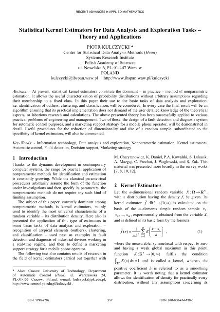
RECENT ADVANCES in APPLIED MATHEMATICS
Statistical Kernel Estimators for Data Analysis and Exploration Tasks –
Theory and Applications
PIOTR KULCZYCKI *
Center for Statistical Data Analysis Methods (Head)
Systems Research Institute
Polish Academy of Sciences
ul. Newelska 6, PL-01-447 Warsaw
POLAND
kulczycki@ibspan.waw.pl http://www.ibspan.waw.pl/kulczycki
Abstract: - At present, statistical kernel estimators constitute the dominant – in practice – method of nonparametric
estimation. It allows the useful characterization of probability distributions without arbitrary assumptions regarding
their membership to a fixed class. In this paper their use to the basic tasks of data analysis and exploration,
i.e. identification of outliers, clustering, and classification, will be considered. In every case the final result will be an
algorithm ensuring that its practical implementation does not demand of the user detailed knowledge of the theoretical
aspects, or laborious research and calculations. The above presented theory has been successfully applied to various
practical problems of engineering and management. Two of these, the design of a fault detection and diagnosis system
for automatic control purposes, and a marketing support strategy for a mobile phone operator, will be demonstrated in
detail. Useful procedures for the reduction of dimensionality and size of a random sample, subordinated to the
specificity of kernel estimators, will also be commented.
Key-Words: - Information technology, Data analysis and exploration, Nonparametric estimation, Kernel estimators,
Automatic control, Fault detection, Decision support, Marketing strategy
1 Introduction
Thanks to the dynamic development in contemporary
computer systems, the range for practical application of
nonparametric methods for identification and estimation
is constantly growing. While the classical parametrical
procedures arbitrarily assume the form of the function
under investigations and then specify its parameters, the
nonparametric methods do not require any such kind of
limiting assumption.
The subject of this paper, currently dominant among
nonparametric methods, is kernel estimators, mainly
used to identify the most universal characteristic of a
random variable – its distribution density. Here also is
presented the application of this type of estimators in
some basic tasks of data analysis and exploration –
recognition of atypical elements (outliers), clustering,
and classification – used next as examples in fault
detection and diagnosis of industrial devices working in
a real-time regime, and then to define a marketing
support strategy for a mobile phone operator.
The following text also contains results of research in
the field of kernel estimators carried out together with
* Also: Cracow University of Technology, Department
of Automatic Control (Head), ul. Warszawska 24,
PL-31-155 Cracow, Poland, e-mail: kulczycki@pk.edu.pl,
http://www.control.pk.edu.pl/kulczycki .
M. Charytanowicz, K. Daniel, P.A. Kowalski, S. Lukasik,
A. Mazgaj, C. Prochot, J. Waglowski, and S. Zak. This
material was presented more broadly in the survey works
[7, 8, 10, 12].
2 Kernel Estimators
Let the n-dimensional random variable X : Ω → R ,
with a distribution having the density f, be given. Its
kernel estimator ˆ n
f : R → [0, ∞)
is calculated on the
basis of the m-elements simple random sample x 1,
x 2 , ..., x m , experimentally obtained from the variable X,
and is defined in its basic form by the formula
m
⎛ x − xi
⎞
f ˆ 1
( x)
= ∑ K⎜
⎟
n
mh ⎝ h
, (1)
⎠
i=
1
where the measurable, symmetrical with respect to zero
and having a weak global maximum in this point,
n
function K : R → [0, ∞)
fulfils the condition
∫ n
K( x)
dx
= 1 and is called a kernel, whereas the
R
positive coefficient h is referred to as a smoothing
parameter. It is worth noting that a kernel estimator
allows the identification of density for practically every
distribution, without any assumptions concerning its
n
ISSN: 1790-2769 257 ISBN: 978-960-474-138-0

RECENT ADVANCES in APPLIED MATHEMATICS
membership to a fixed class. Atypical, complex
distributions, also multimodal, are regarded here as
textbook unimodal. In the multidimensional case this
enables, among others, the discovery of total
dependences between particular coordinates of the
random variable under investigation.
Setting of the quantities introduced in definition (1),
i.e. choice of the form of the kernel K as well as
calculation of the value for the smoothing parameter h, is
most often carried out according to the criterion of
minimum of an integrated mean-square error. Broader
discussion and practical algorithms are found in the
books [8; 22, 23] 1 . In particular, the choice of the kernel
form has no practical meaning and thanks to this it is
possible to take into account primarily properties of the
estimator obtained (e.g. its class of regularity, boundary
of a support, etc.) or aspects of calculations,
advantageous from the point of view of the applicational
problem under consideration. Practical applications may
also use additional procedures, some generally
improving the quality of the estimator, and others –
optional – possibly fitting the model to an existing
reality. For the first group one should recommend the
modification of the smoothing parameter [8 – Section
3.1.6; 22 – Section 5.3.1] and a linear transformation [8
– Section 3.1.4; 22 – Section 4.2.1], while for the
second, the boundaries of a support [8 – Section 3.1.8;
22 – Section 2.10].
Kernel estimators allow effective modeling of the
distribution density – a basic functional characteristic of
random variables. Consequently this is fundamental in
obtaining other functional characteristics and parameters.
For example, if in a one-dimensional case the kernel K is
such chosen that its primitive I( x)
= ∫ x K(
y)
dy
may be
−∞
analytically obtained, then the estimator of the
distribution function
m
⎛ x − xi
⎞
F ˆ 1
( x)
= ∑ I⎜
⎟
m ⎝ h ⎠
(2)
i=
1
can be easy calculated. Next, if the kernel K has (strictly)
positive values, the solution for the equation
F ˆ ( x)
= r
(3)
constitutes the kernel estimator of quantile of the order
r ∈(0,1) . For details and proofs of strong consistencies
see [18].
1 For calculating a smoothing parameter one can especially
recommend the plug-in method in the one-dimensional case [8
– Section 3.1.5; 22 – Section 3.6.1], as well as the crossvalidation
method [8 – Section 3.1.5; 21 – Section 3.4.3] in the
multidimensional. Comments for the choice of kernel may
best be found in [8 – Section 3.1.3; 22 – Sections 2.7 and 4.5].
It is worth mentioning also the possibility of applying
data compensation and dimensionality reduction
procedures – original and useful algorithms can be found
in the book [21 – Sections 2.5 and 3.4]. A specialized
algorithm, based on simulated annealing, and dedicated
to data analysis and exploration procedures found in the
next chapter, is being researched – preliminary results
are presented in the work [19].
3 Data Analysis and Exploration
The application of kernel estimators for recognition of
atypical elements, clustering, and classification will be
subsequently investigated in further sections of this
chapter. In all three cases the n-dimensional random
n
variable X : Ω → R is considered.
The text below also contains material from research
carried out together with M. Charytanowicz, K. Daniel,
and C. Prochot, published in the common works [14-17,
20].
3.1 Recognition of Atypical Elements
In many problems of data analysis, the task of
recognizing atypical elements (outliers) – those which
differ greatly from the general population – arises. This
enables the elimination of such elements from the
available set of data, which increases its homogeneity
(uniformity), and facilitates analysis, especially in
complex and unusual cases. In practice, the recognition
process for outliers is most often carried out using
procedures of statistical hypothesis testing [2]. The
significance test based on the kernel estimators
methodology will now be described.
Let therefore the random sample x 1,
x 2 , K , xm
treated as representative, therefore including a set of
elements as typical as possible, be given. Furthermore,
let r ∈(0,1)
denote an assumed significance level. The
n
hypothesis that ~ x ∈R
is a typical element will be tested
against the hypothesis that it is not, and therefore should
be treated as an outlier. The statistic S : R → [0, ∞)
,
used here, can be defined by
S ( ~ x ) = fˆ( ~ x ) , (4)
where fˆ denotes a kernel estimator of density, obtained
for the random sample x 1,
x 2 , K , xm
mentioned above,
while the critical set takes the left-sided form ( −∞ , a]
,
when a constitutes the kernel estimator of quantile of the
order r (see the text connected with formula (3)),
calculated for the sample f ˆ( x 1 ) , f ˆ( x 2 ), K , f ˆ( x m ) ,
with the assumption that random variable support is
n
ISSN: 1790-2769 258 ISBN: 978-960-474-138-0

RECENT ADVANCES in APPLIED MATHEMATICS
bounded to nonnegative numbers.
3.2 Clustering
The aim of clustering is the division of a data set –
for example given in the form of the random sample x 1,
x 2 , K , x m – into subgroups (clusters), with every one
including elements “similar” to each other, but with
significant differences between particular subgroups [5].
In practice this often allows the decomposition of a large
data set with differing characteristics of elements into
subsets containing elements of similar properties, which
considerably facilitates further analysis, or even makes it
possible at all. The following clustering procedure based
on kernel estimators, taking advantage of the gradient
methods concept [4] will be presented in this section.
Here the natural assumption is made that clusters are
associated to modes – local maximums of the density
kernel estimator fˆ , calculated for the considered
random sample x 1,
x 2 , K , xm
. Within this procedure,
particular elements are moved in a direction defined by a
gradient, according to the following iterative algorithm:
0
x j = x j
x
k+
1
j
= x
k
j
for
j = 1, 2,..., m
(5)
k
∇fˆ(
x j )
+ b
k
fˆ(
x j )
for
j = 1, 2,..., m and
k = 0,1,... , (6)
where b > 0 and ∇ denotes a gradient. Thanks to the
proper choice of form of the kernel K, a suitable
analytical formula for the gradient ∇ fˆ becomes
possible. As a result of the following iterative steps, the
elements of the random sample move successively,
focusing more and more clearly on a certain number of
*
clusters. They can be defined after completing the k -th
step, where
D
k
∑ m
j = i + 1
D
k
*
k means the smallest number k such that
m
1
− −
( x i , x j ) , − = m m
k
∑i
= ∑ j = i + i
k 1 1
Dk
1 d x , x
1 1
j )
− Dk
− 1 ≤ c D 0 , where c > 0 and D0
= ∑ i =
=
d
∑
∑
m m
i = 1 j = i + 1
k
i
k
j
( ,
d ( x , x ) , i.e. they are the sums of
the distances between particular elements of the random
sample under consideration before the beginning of
algorithm (5)-(6) and having performed the (k–1)-th and
k-th steps, respectively.
*
Thus, after k -th step, one should calculate the
kernel estimator for mutual distances of the elements
*
1 k
k
*
k
*
x , x2
, K , xm
(under the assumption of nonnegative
support of the random variable), and next, the value can
be found where this estimator takes on the local
minimum for the smallest value of its argument, omitting
a possible minimum in zero. Finally, particular clusters
are assigned those elements, whose distance to at least
one of the others, is not greater than the above value.
Thanks to the possibility of change in the smoothing
parameter value, it becomes possible to affect the range
of a number of obtained clusters, albeit without arbitrary
assumptions concerning the strict value of this number,
which allows it to be suited to a true data structure.
Moreover, possible changes in the intensity of the
smoothing parameter modification procedure enable
influence on the proportion of clusters located in dense
areas of random sample elements to the number of
clusters on the “tails” of the distribution.
The detailed description of the above procedure can
be found in the papers [14, 15].
3.3 Classification
The application of kernel estimators in a
classification task will be considered now. Let the
number J ∈N \ {0,1 } be given. Assume also, that the
possessed random sample x 1,
x 2 , K , xm
has been
divided into J ∈N \ {0,1 } nonempty and separate subsets
1
x 1 ,
2
x 1 ,
J
x 1 ,
1 1
, , x 2 m 1
x K (7)
2 2
, , x m
x K (8)
2 2
M
J
J
m
x 2 , K , x , (9)
J
J
while ∑ m m
j j = =1
, representing J classes with
features as mutually different as possible. The
classification task requires deciding into which of them
n
the given element ~ x ∈R
should be reckoned [5].
The kernel estimators methodology provides a natural
mathematical tool for solving the above problem in the
optimal – in the sense of minimum for expectation of
losses – Bayes approach. Let thus ˆf 1 , f
ˆ2 , ... , fˆ
J denote
kernel estimators of density calculated for subsets
(7)-(9), respectively, treated here as samples. If sizes
m 1 , m 2,
K ,mJ
are proportional to the “frequency” of
appearance of elements from particular classes, the
considered element ~ x should be reckoned into the class
for which the value
m ˆ1( ~ 1 f x)
, m
ˆ2 ( ~ ), ..., ˆ ( ~
2 f x mJ f J x)
(10)
is the greatest.
ISSN: 1790-2769 259 ISBN: 978-960-474-138-0

RECENT ADVANCES in APPLIED MATHEMATICS
4 Fault Detection
The fault detection and diagnosis problem has lately
become one of the most important challenges in modern
control engineering. Early discovery of anomalies
appearing in the operation of a controlled system, from
an industrial robot to a nuclear reactor, most often allows
serious incidents and even catastrophes to be avoided,
which could save material damage, or loss of human life.
Secondly, confirmation of kind and location of these
anomalies is of fundamental meaning, especially when
supervising large systems like complex chemical
installations, as well as modern ships and airplanes. The
importance of the above actions is multiplied by a
psychological factor expressed by an increased feeling of
safety, as well as – for the producer – prestige and
commercial reputation. Finally, economic reasons often
translate into a significant decrease in running costs,
above all by ensuring the proper technological
conditions as well as rationalizing overhauls and
reducing repairs. Among the many different procedures
used with this aim, the most universal are statistical
methods. This paper presents the concept of a fault
detection system, based on the kernel estimators
methodology, covering:
. detection, so discovery of the existence of potential
anomalies in the technical state of a device under
supervision;
. diagnosis, that is identification of these anomalies;
. prognosis, i.e. warning of the threat of their
occurrence in the near future, together with
anticipated classification.
The procedures presented in Chapter 3 provide a
complete and methodologically consistent mathematical
tool to design an effective fault detection system for
dynamical systems, covering detection, diagnosis, and
also prognosis associated with them.
Assume that the technical state of a device under
supervision may be characterized by a finite number of
as well as the set
x 1,
x , ..., xM
1
x 1 ,
1 1
, , x 2 m 1
2 2 2
x 1 , 2 , , x m2
M
J J J
x 1 , x , , xmJ
J
while ∑ m
j j = =1
n
x 2 , ..., x m , (11) m f ˆ ˆ2 ,...,
quantities measurable in real-time. These will be denoted
in the form of the vector x∈
R , called a symptom
vector. One can interpret this name noting that
symptoms of any occurring anomalies should find the
appropriate reflection in the features of a such-defined
vector. More strictly, it is required that both correct
functioning conditions and any type of diagnosed fault
are connected with the most different sets of values
and/or dissimilar relations between coordinates of the
above vector as possible.
Assume also the availability of a fixed set of values
of the symptom vector, representative for correct
functioning conditions of a supervised device:
x 1,
0
2 , (12)
characteristic in the case of occurrence of anomalies.
From the point of view of transparency of the designed
fault detection system, in particular its function of
diagnosis, it is worth dividing set (12) into J ∈N \ {0,1 }
the most possibly different – in the sense of the values of
particular coordinates of the symptom vector and/or
relations between them – subsets assigned to the
previously assumed types of diagnosed faults:
x K (13)
x K (14)
2 K , (15)
M . Where there is no such division,
one can automatically divide set (12) into subsets
(13)-(15) using the clustering algorithm presented in
Section 3.2, although this then often requires laborious
interpretation concerning each of them.
Fault detection will first be considered. With this aim
the procedure for the recognition of atypical elements,
described in Section 3.1, can be applied. Assume
therefore that the random sample considered there,
including elements treated as typical, constitutes set (11)
representing the correct functioning conditions for a
supervised device, while x ~ denotes its current state.
Applying the above mentioned procedure for the
recognition of atypical elements, one can confirm if the
present conditions should be regarded as typical or rather
not, thus showing the appearance of anomalies.
For fault diagnosis, if one already is in possession of
samples (13)-(15) characterizing particular types of
faults being diagnosed, then after the above described
detection of anomalies, one can – applying directly the
procedure for Bayes classification presented in Section
3.3 – infer which of them is being dealt with. Note that
the range of faults which can be discovered by detection
may significantly exceed all types of faults assumed to
be diagnosed.
Finally, if subsequent values of the symptom vector,
obtained successively during the supervising process, are
available, then it is possible to realize fault prognosis. It
can be carried out by separate forecasts of values of the
function fˆ given by dependence (4) and m ˆf 1 1,
2 m J f J to be seen in formula (10), and
inferences based on these forecasts for detection and
ISSN: 1790-2769 260 ISBN: 978-960-474-138-0

RECENT ADVANCES in APPLIED MATHEMATICS
diagnosis, according to guidelines presented in the
previous two paragraphs. To calculate the values of
forecasts of the functions fˆ , ˆf 1 , f
ˆ2 , ... , fˆ
J it is
recommended to use the classical linear regression
method separately, though in a version enabling easy
updating of a model during successive collection of
subsequent current values of the symptom vector.
Appropriate formulas are found in the book [1 – Chapter
3 and additionally Chapter 4].
The proper operation of the fault detection system
investigated in this section was verified experimentally
for a robust control applied to the task from a field of
robotics [9]. Thus, in cases where the symptoms
appeared abruptly, the anomalies of the device were
promptly discovered and correctly recognized within the
scope of detection and diagnosis. If, on the other hand,
the fault was accompanied by a slow progression of
symptoms, it was forecast with a correct indication of
the type of fault about to occur (scope of prognosis), and
later it was also discovered and identified in detection
and diagnosis. One should underline that fault prognosis,
still rare in practical applications, proved to be highly
effective in the case of slowly progressing symptoms,
discovering and identifying anomalies before the
object’s characteristics transgressed the range for correct
conditions for a system’s functioning, thanks to the
proper recognition of the change in the trend of values of
the symptom vector, which indicates an unfortunate
direction of its evolution.
More details can be found in the paper [13].
5 Marketing Strategy
The highly dynamic growth prevalent on the mobile
phone network market, naturally necessitates a company
to permanently direct its strategy towards satisfying the
differing needs of its clients, while at the same time
maximizing it income. The uncontrollable nature of this
kind of activity, however, can lead to a loss of coherence
in treating particular clients, and their subsequent
defection to competitors. To avoid this a formal solution
of global nature must be found. Below are presented
results of research obtained using statistical kernel
estimators, carried out in the procedures discussed in
Chapter 3. This procedure, prepared for a Polish mobile
phone network operator, concerns long term business
clients, i.e. those with more than 30 SIM cards and an
account history of at least 2 years.
In practice there is a vast spectrum of quantities
characterizing particular subscribers. Following detailed
analysis of the economic aspects of the task under
investigation here, it was taken that basic traits of clients
would be shown by three quantities : average monthly
income per SIM card, length of subscription and number
of active SIM cards. Thus each of m-elements of a
database x 1 , x 2 ,..., x m is characterized by the
following 3-dimensional vector:
⎡ xi,1
⎤
⎢ ⎥
x i = ⎢xi,2
⎥ for i = 1, 2, ..., m , (16)
⎢ ⎥
⎣xi,3
⎦
where x i, 1 denotes the average monthly income per SIM
card of the i-th client, x i, 2 – its length of subscription,
and x i, 3 – the number of active SIM cards.
In the initial phase, atypical elements of the set x 1 ,
x 2 ,..., x m (outliers) are eliminated, according to the
procedure presented in Section 3.1. The uniformity of
the data structure is so increased, and it is worth
underling, this effect is obtained by canceling only those
elements which would not be of importance further in
the procedure investigated.
Next clustering of the data set is performed, using the
algorithm as shown in Section 3.2. This results in a
division of the data set representing specific clients, into
groups of similar nature. This should be followed by
another, albeit slightly different, elimination of atypical
elements, achieved by removing clusters with small
numbers of elements. As well as omitting information of
little significance, it is also in order to improve
conditions for the classification algorithm applied at a
further stage of the procedure worked out – kernel
estimators calculated on the basis of an insufficient
number of samples (7)-(9) may not be representative.
Next for each of the above defined clusters, an
optimal – from the point of view of expected profit of
the operator – strategy is created for treating subscribers
belonging to it. With regard to the imprecise evaluation
of experts used here, elements of fuzzy logic [6] and
preference theory [3] have been used – details are
however beyond the scope of this paper.
It is worth pointing out that none of the above
calculations must be carried out at the same time as
negotiating with the client, but merely updated (in
practice once every 1-6 months).
The client being negotiated with is described with the
aid of three quantities, in reference to formula (16) given
here as:
⎡
~
x1
⎤
~
x =
⎢~
⎥
⎢
x2
⎥
, (17)
⎢~
⎣x3
⎥⎦
where
~ x 1 denotes its average monthly income per SIM
card,
~ x 2 – length of subscription, and
~ x 3 is the number
ISSN: 1790-2769 261 ISBN: 978-960-474-138-0

RECENT ADVANCES in APPLIED MATHEMATICS
of active SIM cards of that client. This data can relate to
the subscriber history to date in a given network, when
renegotiating contract terms, or in a rival network if
attempting to take them over. Classification to the proper
subscriber group, from those obtained as a result of
clustering, is achieved with the procedure presented in
Section 3.3. To this purpose, first kernel estimators are
calculated separately for each cluster. In classification
element (17) is mapped to the class (cluster), for which
the value m ˆ1( ~
1 f x)
, m
~
),..., ˆ (
~
2 fˆ2 ( x mJ f J x)
to be seen in
formula (10), is greatest. Due to the fact that the
marketing strategies for particular clusters have already
been defined, this finally completes the procedure for the
algorithm to support the marketing strategy for a
business client, investigated here.
The above method was successfully implemented for
the needs of a Polish network operator. In relation to the
comment at the end of Section 3.2, the intensity of the
smoothing parameter modification procedure was
somewhat lessened with respect to the optimal in the
mean-square sense, with the aim of dividing the largest
cluster and decreasing the number of peripheral clusters.
Finally, two large clusters containing 27% and 23% of
elements, two medium of 14% and 7%, and 22 small
each including less than 3% – the most uncommon
firms, were obtained.
More details can be found in the papers [16, 17].
References:
[1] Abraham B., Ledolter J., Statistical Methods for
Forecasting, Wiley, 1983.
[2] Barnett V., Lewis T., Outliers in Statistical Data,
Wiley, 1994.
[3] Fodor J., Roubens M., Fuzzy Preference Modelling
and Multicriteria Decision Support, Kluwer, 1994.
[4] Fukunaga K., Hostetler L.D., The estimation of the
gradient of a density function, with applications
in Pattern Recognition, IEEE Transactions on
Information Theory, Vol. 21, 1975, pp. 32-40.
[5] Hand J.H., Mannila H., Smyth P., Principles of Data
Mining, MIT Press, 2001.
[6] Kacprzyk J., Zbiory rozmyte w analizie systemowej,
PWN, Warszawa, 1986.
[7] Kulczycki P., Applicational Possibilities of
Nonparametric Estimation of Distribution Density
for Control Engineering, Bulletin of the Polish
Academy of Sciences; Technical Sciences, Vol. 56,
2008, pp. 347-359.
[8] Kulczycki P., Estymatory jadrowe w analizie
systemowej, WNT, 2005.
[9] Kulczycki P., Fuzzy Controller for Mechanical
Systems, IEEE Transactions on Fuzzy Systems, Vol.
8, 2000, pp. 645-652.
[10] Kulczycki P., Estymatory jadrowe w badaniach
systemowych, in: Techniki informacyjne w badaniach
systemowych, Kulczycki P., Hryniewicz O.,
Kacprzyk J. (eds.), WNT, 2007, pp. 79-105.
[11] Kulczycki P., Kernel Estimators in Industrial
Applications, in: Soft Computing Applications in
Industry, Prasad B. (ed.), Springer-Verlag, 2008, pp.
69-91.
[12] Kulczycki P., Nonparametric Estimation for Control
Engineering, in: Proc. 4th WSEAS/IASME International
Conference on Dynamical Systems and Control,
Corfu, 26-28 October 2008, pp. 115-121.
[13] Kulczycki P., Statistical Kernel Estimators for
Design of a Fault Detection, Diagnosis and Prognosis
System, The Open Cybernetics and Systemics
Journal, Vol. 2, 2008, pp. 180-184, open access:
http://www.bentham.org/open/tocsj/openaccess2.htm.
[14] Kulczycki P., Charytanowicz M., A Complete
Gradient Clustering Algorithm Formed with Kernel
Estimators, Applied Mathematics and Computer
Science, 2010, in press.
[15] Kulczycki P., Charytanowicz M., Kompletny
algorytm gradientowej klasteryzacji, in: Sterowanie i
automatyzacja: aktualne problemy i ich rozwiazania,
Malinowski K., Rutkowski L. (eds.), EXIT, 2008, pp.
312-321.
[16] Kulczycki P., Daniel K., Algorytm wspomagania
strategii marketingowej operatora telefonii komorkowej,
in: Badania operacyjne i systemowe 2006: metody i
techniki, Kacprzyk J., Budzinski R. (eds.), EXIT,
2006, pp. 245-256.
[17] Kulczycki P., Daniel K., Metoda wspomagania
strategii marketingowej operatora telefonii
komorkowej, Przeglad statystyczny, 2009, in press.
[18] Kulczycki P., Dawidowicz A.L., Kernel estimator
of quantile, Universitatis Iagellonicae Acta
Mathematica, Vol. XXXVII, 1999, pp. 325-336.
[19] Kulczycki P., Lukasik S., Redukcja wymiaru i
licznosci proby dla potrzeb syntezy statystycznego
ukladu wykrywania uszkodzen, in: Systemy
wykrywajace, analizujace i tolerujace usterki,
Kowalczuk Z. (ed.), PWNT, 2009, pp. 139-146.
[20] Kulczycki P., Prochot C., Wykrywanie elementow
odosobnionych za pomoca metod estymacji
nieparametrycznej, in: Badania operacyjne i
systemowe: podejmowanie decyzji – podstawy
teoretyczne i zastosowania, Kulikowski R., Kacprzyk
J., Slowinski R. (eds.), EXIT, 2004, pp. 313-328.
[21] Pal S.K., Mitra P., Pattern Recognition Algorithms
for Data Mining, Chapman and Hall, 2004.
[22] Silverman B.W., Density Estimation for Statistics
and Data Analysis, Chapman and Hall, 1986.
[23] Wand M.P., Jones M.C., Kernel Smoothing.
Chapman and Hall, 1994.
ISSN: 1790-2769 262 ISBN: 978-960-474-138-0