Conveyor Belt System Design

Edition
Conveyor Belt System Design
CONTI Conveyor Belt Service Manual
ContiTech Division of Continental AG

Conveyor Belt Service Manual
ContiTech
Specialist in rubber and
plastic technology
Conveyor Belt
System Design
Edited by:
Dr.-lng. Rainer Alles
Contributors:
Obering. W. Ernst
Prof. Dr.-lng. W.S.W. Lubrich and
the following
ContiTech engineers
Dr.-lng. R. Alles
Dipl.-lng. G. Bottcher
Dipl.-lng. H. Simonsen
Dipl.-lng. H. Zintarra
Published by
ContiTech Transportbandsysteme GmbH
D-30001 Hannover, Germany
Status 1994
a reversed version will be available
at autum 1995
The ContiTech Group
is a development partner and
original equipment manufacturer
for numerous branches
of industry with high grade
functional parts, components
and systems It is part of
the Continental Corporation
with over 26 companies in
Europe specialising in rubber
and plastics technology
and utilising their common
know-how.
That's what the ContiTech
brand is all about.

Table of Contents
Page
1 Basic expressions and definitions ................. 6
2 Stipulation of principal data .......................... 9
2.1 Material handled.......................................... 10
2.2 Flolw of material handled ........................... 12
2.3 Conveying track .......................................... 13
2.4 Type of belt conveyor.................................. 14
2.4.1 Belt width .................................................... 15
2.4.2 Belt speed ................................................... 16
2.4.3 Belt support ................................................. 18
2.5 Conveying capacity ..................................... 20
3 Calculation of belt conveyor ........................ 27
3.1 Masses........................................................ 29
3.1.1 Idlers............................................................ 30
3.1.2 Conveyor belt .............................................. 32
3.1.3 Drive elements ............................................ 33
3.2 Coefficients................................ ................. 34
3.3 Motional resistance of sections ................... 36
3.4 Required power........................................... 41
3.5 Peripheral force........................................... 44
3.5.1 Starting and stopping .................................. 47
3.5.2 Multiple pulley drive..................................... 50
3.6 Calculation example ................................... 53
4 Stipulation of tgension member ...................56
4.1 Belt tensions................................................ 61
4.1.1 Belt tensions in operation............................ 66
4.1.2 Belt tensions on starting and stopping ........ 68
4.1.3 Belt tensions with regard to sections............70
4.2 Additional strains ......................................... 71
4.2.1 Flat-to-trough transition and vice versa....... 73
4.2.2 Transition curves ......................................... 75
4.2.3 Turnover .......................................................77
4.3 Selection criteria.......................................... 78
4.3.1 Pulley diameter.............................................79
4.3.2 Troughing properties ................................... 81
4.3.3 Centre distance and takeups ...................... 82
4.3.4 Effects of material handled.......................... 83
Page
4.3.5 Feeding strain.............................................. 85
4.4 Tension member data ................................ 87
4.4.1 Textile tension members ............................. 90
4.4.2 Steel cable tension members...................... 91
4.4.3 Splice dimensions ....................................... 92
5 Selection of covers ..................................... 96
5.1 Cover material ............................................ 98
5.2 Cover gauge ............................................. 100
5.2.1 Abrasion resistance................................... 101
5.2.2 Impact resistance ...................................... 102
5.3 Special cover structures ........................... 103
6 Steep angle conveyor belts ...................... 105
6.1 Chevron cleated belt ................................ 107
6.2 Box-section belt ........................................ 108
6.2.1 Conveying capacity ................................... 110
6.2.2 Constructional data ................................... 111
6.3 Fin-type belt and belt with
bonded partitions ...................................... 113
7 Elevator-belts ................................ ........... 115
7.1 Conveying capacity .................................. 116
7.2 Power requirement and belt tensions........ 117
7.3 Selection of bucket elevator belts ............ 119
7.3.1 Tension member ....................................... 120
7.3.2 Covers ....................................................... 122
7.3.3 Buckets and bucket attachments .............. 123
8 Piece goods handling
and belts for sliding bed operation ............ 125
8.1 Conveying capacity .................................. 126
8.2 Calculation of required power ................... 127
8.3 Conveyor belt desing................................. 129
9 Appendix ........................................ .......... 130
9.1 Index ......................................................... 131
9.2 Symbols .................................................... 134
9.3 Questionnaires ...........................................
9.4 Printed forms for calculation.......................

An insignificant side-note for all those who are already accustomed to
using Sl units or units derived from them and who take advantage of this
"standard" settlement by the international units system.
For all other readers it is pointed out that an "Act on Units in Measuring
Procedure", regulating the use of technical units in business and official
transactions, was passed on 2nd July 1969 and became mandatory for
us when the transitional period expired on 1st January 1978.
The effects of this Act on materials handling technology are minimal as
most of the units already widely used in this sphere have undergone no
change. One essential point is the uniform stipulation of the
kilogram (kg) as a unit for mass
It was furthermore stipulated that the word "weight" may be used only as
a mass quantity. The weights listed in a large number of tables and
reference books thus retain their numerical value. Other units of weight or
of mass are the gram (g) and the ton (t).
We recall: one kilogram was accelerated by the gravitational attraction of
the earth at approx. 9.81 m/s 2 and thus exercised on the base it is resting
upon a weight of one kilogram-force. In the Space Age we now depart
from this unit of force, that applied solely under the gravitational
conditions of the earth, and use exclusively the
Newton (N) as a unit for force
One kilogram is accelerated by one Newton at 1 m/s 2 or one kilogram
acts under the influence of the acceleration due to gravity on its base
with the force of approx. 9.81 Newton. All forces that were formerly
expressed in kilogram-force attain a numerical value increased approximately
by the factor 10 with Newton as a unit.
The breaking strength of a conveyor belt in kilogram-force related to the
unit of width in cm retains approximately its familiar numerical value if the
breaking strength in N is related, as practised below, to the width in mm.
1 kilogram-force/cm ≈ 1 N/mm
It follows from the introduction of the Newton as a unit for force that the
acceleration due to gravity g occurs in all calculation formulae in which
weights are determined or other forces with their origin in weights are
calculated. For this purpose
Acceleration due to gravity g = 9,81 m/s 2
can be inserted with sufficient accuracy. A simplification results in the
calculation of power in W (Watt) by the multiplication of force in N and
speed in m/s. A conversion factor is then superfluous.
This short introduction is aimed at drawing your attention to the
changeover resulting from these regulations for the following calculation
principles and data.
2

D - Conveyor belt calculation D
This section of the ContiTech Conveyor Belt Service Manual comprises
design fundamentals and data essential for the designing of a conveyor
belt system. The calculation procedures and data stated take the current
level of technology largely into account with regard to the latest research
results and independent tests, provided that these give sufficiently wellfounded
information. Advice is given to enable the appropriate conveyor
belt from the Conti-range to be selected for each individual project and to
help both the designer and the user to attain optimum coordination
between the conveyor belt, the design of the beltsystem and the practical
application.
The calculation of the belt conveyor for bulk material set out at the
beginning of these calculation principles is based on specifications
contained in DIN standard 22101 (February 1982) and is supplemented
by extending design procedures. Essential calculation stages not included
in the DIN 22101 standard specifications have been described for
instance in publications by Vierling *
The designations of formula quantities have been adapted as far as
possible to general guidelines. Designations already well known from
technical literature in this field have also been used, however, where we
felt them to be beneficial.
Only the "statutory units" (Sl units or units derived therefrom) on which
the "International Units System" (Sl) is based are used in the formulae,
tables and diagrams. To facilitate comprehension, the units used in the
further course of the calculation are stated after the respective formulae,
whereby the units listed in the index of symbols are to be used. A brief
dimensional consideration helps in cases of doubt. The units to be used
are stated in the case of formulae with conversion factors or dimensionaffected
constants.
*
Vierling, A Zum Stand der Berechnungsgrundlagen fur Gurtforderer Braunkohle Warme und Energie
19 (1967) No 9,P 309-315
Vierling, A Zur Theorie der Bandförderung Continental-Transportband-Dienst 1972, 3rd edition.
3

D
In general, the following data are known before a belt conveyor is
designed:
Type of material to be conveyed
(e. g. bulk weight, lump size, angle of repose)
Flow of material to be conveyed (e. g. mass flow, volume flow)
Conveying track (e. g. conveying length, conveying height).
These data are a basis for selection of the type of belt conveyor and thus
for the type of conveyor belt. The decision on whether it is a plain
standard conveyor belt, a steep-angle conveyor belt or a special
conveyor with the corresponding special-purpose belt serves as a
reference point for the stipulation of the principal data, in particular of
conveying speed and belt width, but may necessitate for instance in
addition the stipulation of the troughing design, the belt surface profile or
the pitch of elevator buckets.
The next factors to be determined are motional resistances and required
power of the belt conveyor. If the design is already established, it is the
size, position and type of the driving motors that have to be recorded
besides the data stated hitherto, as these may have a decisive influence
on the selection of the conveyor belt. The calculation of the belt
conveyor leads on to the peripheral forces at the driving pulleys. Their
magnitude depends on the extent of the motional resistances but varies
for temporary operating conditions such as starting and stopping.
The design of the tension member in the conveyor belt then follows. Its
tensile strength is determined mainly by the magnitude of the belt
tensions. Further influences result from a variety of criteria relating to
operation and design.
As the strength of the tension member must always have a specific
safety margin over the maximum stress, it is essential to stipulate the
safety coefficient or to check the available safety margin on selection of
the tension member. Special attention must be paid here to the durability
of the conveyor belt at the joints.
The tension member of the conveyor belt is enclosed in the covers, which
thus form an effective protection against external influences. For this
reason the material and construction are selected to counteract the
effects of the material conveyed and of the environment. Conformity to
the tension member must also be observed on selection of the covers.
Conti conveyor belts are supplied to all parts of the world, using those
dispatch facilities best suited to the destination; the packaging
guarantees safe transport even in exceptional cases. The optimum part
lengths can be determined for each particular instance to provide
inexpensive shipment and simple assembly. The thickness, width and
weight of the belt are to be given special consideration.
The conveyor belt calculation process described also conforms with the
arrangement of the following chapters. The chart shows both the normal
sequence of design stages and the feasibility of starting at any section,
provided that specific data or parameters are known. In general the
single chapters go deeper into the respective subject with increasing subdivision,
so that a rough assessment of the belt structure can be made by
consulting the general chapter alone. Special reference is made to those
calculation points at which an assessment is recommended.
4

Basic expressions and definitions D - 1 D
Stipulation of principal data D - 2
Material handled ............. 2.1
Flow of material 2.2 Conveying track............. 2.3
Type of belt conveyor ..... 2.4
Conveying capacity ........ 2.5
Calculation of belt conveyor D - 3
Masses ........................... 3.1
Coefficients 3.2 Motional resistance ....... 3.3
Required power .............. 3.4
Peripheral forces............. 3.5
Calculation example ....... 3.6
Stipulation of tension member D - 4
Tensile forces of belt ...... 4.1
Additional strains 4.2 Selection criteria............ 4.3
Tension member data..... 4.4
Selection of covers D - 5
Cover material 5.1 Cover gauge.................. 5.2
Special cover structures...................... 5.3
Steep-angle conveyor belts D - 6
Elevator belts D - 7
Piece goods handling and belts for sliding bed operation D - 8
Appendix D - 9
The staff of the ContiTech Transportbandsysteme GmbH with its
sophisticated research and development resources is available for direct
consultation and to answer any questions.
Please address enquiries to:
ContiTech Transportbandsysteme GmbH
Postfach 169, D-30001 Hannover
Büttnerstraße 25, D-30165 Hannover
Telefon (0511)938-07
Telefax (0511)938-2580
Telex 92170 con d
The computer programmes filed in the constantly expanding library of the
Department for Application Technique enable enquiries to be dealt with
promptly Apart from specific individual problems, this facility permits
above all extensive calculations and design alternatives to be
investigated without loss of time Reference can be made to the currently
complied programmes at those points of the conveyor belt calculation
marked with the key word 'CONTI-COM'.
5

D - 1 D - 1 Basic expressions and definitions
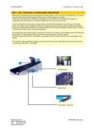
Continuous conveyors: Continuous conveyors are mechanical, pneumatic
and hydraulic conveying devices with which the material to be
handled can be moved continuously on a fixed conveying track of
restricted length from feeding point to discharge point, possibly at
varying speed or in a fixed cycle. These conveyors are available in
stationary or mobile versions and are used for the handling of bulk
materials or piece goods.
Belt conveyors: Continuous conveyors whose belts have a tension
member consisting of synthetic fabrics or steel cables with rubber or
synthetic covers; the belts are supported by straight or trough-shaped
idlers or have sliding support on a smooth base as a tension and support
member. The actual conveying is done on the top run, in special cases
on the top run and the return run. Belts with cleated top covers, specialpurpose
belts or sandwich belts are used for steep-angle conveying.
11 10 1 13 8 6 12 2
17 5 15 7 9 16 4 3 14
1 Feed
2 Discharge
3 Head pulley (drive pulley)
4 Snub or deflecting pulley
5 Tail pulley (takeup pulley)
6 Top run (tight side)
7 Return run (slack side)
8 Rop run idlers
9 Return run idlers
10 Feed rollers
11 Flat-to-trough transition
12 Trough-to-flat transition
13 Feed chute
14 Belt cleaner (transverse scraper)
15 Belt cleaner (plough-type scraper)
16 Drive unit
17 Counterweight
Belt-type elevators: Continuous conveyors with buckets or similar
containers as carriers; these either scoop the material or are filled by
metering hoppers and emptied at specific discharge points. The tension
unit consists of belts to which the containers are attached. Transport is
effected at any angle from vertical to horizontal.
Flow of material: Mass or volume of the conveyed bulk material or piece
goods per unit of time in continuous conveying. In contrast, the capacity
is not time-related.
Conveying capacity: The volume capacity or capacity of material
conveyed that can be attained with the given conveying speed and the
available cross-section area or the container volume and spacing.
6

Conveying speed: Speed of the material conveyed. The conveyor belt
as the support member determines the speed of the material on it.
Centre distance: The distance between head and tail pulley of the
conveyor. The belt length as the inside circumference of the endless,
slack belt results from this distance only when the pulley circumference
and any belt loops (tension loops, discharge loops etc.) present are taken
into account.
Conveying length: The distance between the centre of the material
feeding point and the axle of the discharge pulley. If the material
conveyed is stripped off, the centre of the material discharge is to be
taken instead. In general the conveying length is approximately equal to
the centre distance. The conveying length may, however, besmallerthan
the centre distance or be variable during the conveying process.
D - 1
Conveying height: The difference in height between material feed and
material discharge. Belt conveyors with sections at different gradients
yield the section heights allocated to the section lengths.
Belt support: The belt is generally supported by fixed idlers or by
suspended idlers. The belt can be flat or troughed by multi-roll idlers.
Troughing permits a greaterflow of material and promotes improved belt
training. The idler spacing is normally larger on the return run than on the
top run and can also be graduated within one belt conveyor. Special idler
designs or arrangements are frequently selected at the feeding points
and for belt cleaning.
Flat belt V-trough 3-roll troughing
(with CONTIWELL ® -side wall)
Square-troughing belt
5-part troughing
Conveyor belt: The task of the conveyor belt is to carry the material
handled and simultaneously to transmit the driving forces to overcome
the motional resistances. The conveyor belt consists in general of the
tension member and the top and bottom covers, which form a coreprotecting
covering.
Those conveyor belts used in belt conveyors are to be regarded as
continuous conveying elements composed of one or more belt sections
joined together at their ends. Short conveyor belts can also be
manufactured in endless versions.
7

D - 1
Steep angle conveyor belts: Rollback of the material handled can be
prevented by means of chevron cleats, fins or cross partitions on the
carrier side when the conveying gradient is steep. The design can be
adapted to the material to be conveyed and to the transverse stability
required. Cross partitions and corrugated sidewalls can be combined to
form the corrugated box-section belt.
Steep angle
conveyor belt with HÖCKER ® CONTIWELL ®
chevron cleats Conveyor belt Box-section belt
Elevator belts: These are used in belt-type bucket elevators and are
provided with special brackets for the attachment of containers, buckets
or belt slings.
Tension member: The task of the tension member is to transmit the
forces induced at the drives for overcoming the system resistances to the
point where they are needed. In the fabric ply belt, the tension member
consists of one or more plied fabrics. In the case of a steel cable belt, the
tension member consists of steel cables arranged on a single plane and
running parallel to each other longitudinally; these cables are imbedded
in core rubber.
Core rubber: The core rubber envelops the steel cables of the steel
cable tension member, providing good adhesion to the cover material
with a high dynamic carrying capacity. The physical properties are
maintained even after repeated curing, for instance on splicing.
Belt covers: The covers protect the tension member from damage and
other environmental influences. The top and bottom covers may vary in
thickness. The bottom cover can be omitted from bare-bottom-ply belts
for sliding bed operation. Additional elements designed to increase
impact resistance or for monitoring purposes may be located in the
covers. The cover materials can be selected to suit any application.
Surface patterning: For improved holding of materials on gradients or
for special applications, the top cover can be manufactured in a patterned
or a cleated version.
8

D - 2 Stipulation of principal data D - 2
Material handled 2.1
Flow of material handled 2.2 Conveying track 2.3
Type of belt conveyor 2.4
Belt width 2.4.1
Belt speed 2.4.2 Belt support 2.4.3
Carrying capacity 2.5
The designing of a conveyor belt begins with an investigation into the
service requirements and the stipulation of the principal data characterizing
the specific application. Data already available can be checked
against the guide values stated in this section.
The optimum conveyor belt cannot be selected by means of the principal
data alone, as the operating method and the belt conveyor design also
have a considerable influence. If the stress and strain on the conveyor
belt are not known in detail, a calculation of the belt conveyor must be
executed with reference to the bulk material transport up to approx. 30°
system gradient in section D - 3. Sections D - 6 to D - 8 contain
supplementary data for the calculation of steep-angle conveyors for bulk
materials, of elevators and piece goods conveyors.
9

D – 2.1
D - 2.1 Material handled
The physical and chemical properties of the material to be handled must
be taken into account when selecting the belt conveyor and designing the
conveyor belt.
Properties of material to be handled (guide values)
Material to be handled
Ammonium sulphate
Artificial fertilizers
Ash, dry
Ash, wet
Asphalt, crushed
Bauxit, crushed
Bauxit, fine
Berry und Lorraine iron, fine
Beet
Beet chip, wet
Blast furnace slag
Cement
Cereals (not oats)
Clay, damp
Clinker
Coal, fine
Coal, raw
Coke
Concrete, wet
Copper ore
Crushed rock
Felspar, crushed
Fish meal
Flour
Foundry sand
Foundry waste
Fruit
Glass, crushed
Granite, crushed
Graphite, powder
Gravel and sand, wet
Gravel, graded, washed
Gravel, ungraded
Gypsum, crushed
Gypsum, powdered
Bulk
density
in t/m 3
0.75-0.95
0.9-1.2
0.65-0.75
0.9
0.7
1.2-1.4
1.9-2.0
3.2
0.65-0.75
0.5
1.2-1.4
1.2-1.5
0.7-0.85
1.8
1.2-1.5
0.8-0.9
0.75-0.85
0.45-0.6
1.8-2.4
1.9-2.4
1.5-1.8
1,6
0.55-0.65
0.5-0.6
1.2-1.3
1.2-1.6
0.35
1.3-1.6
1.5-1.6
0.5
2.0-2.4
1.5-2.5
1.8
1.35
0.95-1.0
Angle
of
repose
in °
12
15
15
10
18
0-10
10-12
15-18
10-15
10
18
15
0-5
15
10-15
15
10
15
18
15
Max.
gradient
of fight
δ
22
12-15
16
18
22
18-20
18
18
15-17
15-17
18
15-20
14
18-20
18
18-20
18
17-18
16-22
18
16-20
18
25
15-18
20
16
12-15
12-15
20
20
20
12-15
18-20
18
23
mech.
Possible effect
+ + +
Household refuse 0,6 18-20 + +
Iron ore
Iron ore, pellets
Lignite briquettes oval
Lignite, dry
Lignite, wet
Lime, lumps
Limestone, crushed
Maize
Manganese
Matchwood
Oil cake
Oil sand
Overburden
Peat
Phosphate, crushed
Phosphate, fine
Potash
1.7-2.5
2.5-3.0
0.7-0.85
0.5-0.9
0.9
1.0-1.4
1.3-1.6
0.7-0.75
2.0-2.2
0.2-0.35
0.7-0.8
1.6-1.8
1.6-1.7
0.4-0.6
1.2-1.4
2.0
1.1-1.6
15
12
15
15
15-20
15
15
12
15
10
15
15
15
12-15
15
18
15
+ +
+
+ +
+ +
+
++
++
++
++
+ +
+
++
++
++
++
12-13
15-17
18-20
15-20
16-18 +
15
18-22
22-24
++
15
20
17 ++
16
18-20
18
18
chem. temp.
+
+
+
+
++
++
+
++
++
++
+ +
+
+
+
++
+
+ +
10

Material to be handled
Rock salt
Rubber, pellets
Salt, coarse
Salt, fine
Sand, dry
Sand, wet
Sandstone, crushed
Scrap metal
Slag
Slate, crushed
Sludge
Soap flakes
Soil, damp
Sugar cane
Sugar, raw
Sugar, refined
Bulk
density
in t/m 3
1.2
0.8-0.9
1.2
1.2-1.3
1.3-1.4
1.4-1.9
1.3-1.5
1.2-2.0
1.3
1.4-1.6
1.0
0.15-0.35
1.5-1.9
0.2-0.3
0.9-1.1
0.8-0.9
Angle
of
repose
in °
Max.
gradient
of fight
δ
15 18
12
15
15
15
15
0
15-20
18-20
15-18
16-20
20-25
18
15
18-20
15
20
Timber, pieces 0.25-0.5 20-25
mech.
+
++
+
++
++
++
+
+
Possible effect
chem. temp.
+
+
+
+
D – 2.1
Key:
+ medium wear + + heavy wear
chemically aggressive
chemically highly aggressive
temperatures above 70° temperatures above 120°C
The dynamic angle of repose is in general lower than the natural angle of
incline of the material handled and depends on
the type of material handled,
the conveying speed,
the design of the feeding point and
the gradient of the system.
It permits an assessment of the cross-sectional form of the bulk material
on the belt. The maximum gradient stated for the flight applies to a
standard, uncleated belt surface.
11

D – 2.2
D - 2.2 Flow of material handled
If a specific quantity of material is to be handled in a prescribed time, the
Mass flow Q m
results with the mass of the material handled, and the
Volume flow Q V =Q m /
for bulk materials with bulk density .
in t/h
in m³/h.
The necessary conveying capacity of the conveyor belt or belt conveyor
to be selected is determined by these two values. To what extent
downtime may occur through maintenance, breakdown and repairs and
to operation-related interruptions in conveying must be taken into account
when making the selection.
Operating hours per year
Working days per year 1 shift* 2 shifts 3 shifts
365
250
200
2920
2000
1600
5840
4000
3200
8760
6000
4800
* 1 shift = 8 hours
Guide values for maximum material flows
Belt conveyors
Steep angle conveyor belts
Elevators
QV in m³/h
approx. 25.000
approx. 1.400
approx. 1.500
Qm in t/h
approx. 40.000
approx. 3.000
approx. 2.500
12

D - 2.3 Conveying track D – 2.3
Owing to its continuous conveying process, the belt conveyor has
relatively low flight loads and can consequently be adapted to any
routing. The belt gradient can be changed at random, which may provide
the most economic solution for longhaul conveying systems in particular.
Certain minimum radii of the concave or convex curves must be adhered
to. Laying in horizontal curves is also feasible with belt conveyors. The
use of a high-strength tension member permits considerable conveying
lengths and conveying heights to be attained. Centre distances in the
magnitude of 5 to 10 kilometers and conveying heights of up to several
hundred meters are no longer a rarity.
Belt conveyors with steep angle belts are normally designed for shorter
flights at a very steep gradient. The belt guidance can be adapted largely
to the specific application in this case too with the use of appropriate
supporting elements.
Belt elevators are used almost exclusively for vertical transport with
conveying heights of up to almost 100 meters. The operating principle
permits no curves or significant gradients in the flight. The use of steep
angle conveyor belts and elevator belts overlaps in the range of very
steep to vertical transport. Individual adaptation of the conveyor element
is frequently essential in this instance.
13

D – 2.4
D - 2.4 Type of belt conveyor
The transport of bulk material and piece goods on conveyor belts with no
surface partitioning or on hugger belts is restricted by the gradient at
which the material being handled begins to slip or to roll. Nor is faultless
transport guaranteed if starting or stopping induces this process. The
critical conveying gradient angle for a smooth belt is between 15° and 20°
for the majority of different types of material handled. Furthermore,
special belts permitting steeper gradients have to be used. The stated
guide values apply to ascending transport.
1 Conveyor belts with no surface partitioning
(Conveyor belts with cover patterning for bulk materials)
2 Piece goods conveyor belts with cover patterning , Rollgurt *
3 Belts with chevron cleats
4 Fin belts, box-section belts with corrugated sidewalls
5 Conveyor belts in sandwich design
6 Elevator belts
The maximum gradients are to be selected on the small side, if easily
flowing bulk material is to be conveyed at an angle on conveyor belts of
groups 1,2 or 3. With increasing surface pattern depth and with transport
in buckets etc., the type of material handled is of essential significance
only with regard to granularity or piece size.
The velocity data, too, represent guide values that are intended to help in
selecting the appropriate type of belt but have to be determined more
precisely in the subsequent design. If a steep angle conveyor belt or an
elevator belt is found to be suitable for the application or if belts for piece
goods or for sliding bed operation are to be designed, special attention
should be paid to the information in the relevant chapters.
For bulk material transport on conveyor belts with cover patterning
(group 1) the maximum conveying gradients can be set approx. 5° higher
than corresponding to the respective angle of the material concerned.
If a control of all requirements has led to the selection of a conveyor with
a belt from groups 2 to 6, the layout information given for these special
conveyor belts in Sections D - 6, D - 7 und D - 8 is to be observed.
*
Tubular belt, developed by Continental and PWH AS (please ask for special literature).
14

Standard belt widths * 300 400 500 600 650 800
D - 2.4.1 Belt width D – 2.4.1
The belt width should be selected as far as possible from standardized or
customary widths as the dimensions of the idlers and other constructional
elements of the belt conveyor are coordinated with these widths.
Belt width B
1000 1200 1400 1600 1800
in mm 2000 2200 2400 2600 2800
3000 3200
In the case of troughed belts, the belt width must not fall short of certain
dimensions, depending on the lump size (edge length) of the material to
be handled, as the material can otherwise not be transported safely. With
strongly eccentric pieces there is furthermore the risk of the belt
mistracking and of idlers being damaged by material projecting beyond
the belt.
Minimum belt widths
Size k of lumps
in mm
Mind. belt width B
in mm
100 400
150 500
200 650
300 800
400 1000
500 1200
550 1400
650 1600
700 1800
800 2000
This data applies to approximately cubic lumps. Narrower widths are also
admissible for oblong lumps (so-called "slabbies") or when single pieces
are imbedded in mainly fine material.
It is to be observed that the troughability too is influenced by the belt
width. The troughability decreases with diminishing belt width. On final
determination of the belt structure, the troughability (D - 4.3.2) is to be
checked.
*
CONTINENTAL conveyor belts are currently available in widths of up to 6400 mm. Textile carcass
belts are available from stock in widths of 400 to 1000 mm.
15

D – 2.4.2
D - 2.4.2 Belt speed
The selection of the belt speed is of decisive significance for the further
designing of the belt conveyor and of the belt.
Application features
Special cases, process-related
(e. g. cooling conveyors)
Small flows of material, protective transport
(e. g. coke bench conveyors)
Standard application conditions and material
handled
(e. g. gravel conveyance)
Large flows of material, long conveying lengths
(e. g. overburden conveyance)
Special cases
(e. g. jet conveyors)
Conveying speed
v in m/s
0.5
0.5-1.5
1.5-3.5
3.5-6.5
6.5 and more
In general a more economic design can be achieved with higher
conveying speeds. The greater the conveying lengths and thus the belt
lengths, the more significant this is, so that maximum conveying speeds
will be selected especially in such cases. The limits imposed first and
foremost by the type and nature of the material to be handled can be
exceeded in many instances if, for example, additional measures are
taken at the feeding points to eliminate or diminish the drawbacks of high
conveying speeds.
Bulk material features
strongly abrasive
fine and light
fragile
coarse grained (sized) and heavy
slightly abrasive
medium bulk weight
medium granularity (unsized)
low conveying
speeds
higher conveying
speeds
Increased conveying speed results in an increased conveying capacity
with a constant belt width. It may thus be possible to select a narrower
belt width or a simpler troughing design for a given flow of material. In
addition, reduced drive tractions and consequently reduced dimensioning
of all elements constituting the belt conveyor may result. Drawbacks are
increased belt wear, to which special attention should be paid in short
belt conveyors, an increased risk of damage to the material handled and
increasing power requirements for large capacities.
Reduced conveying speed correspondingly results in a larger belt width
or a higher-capacity troughing design with the given flow of material. The
increased drive tractions are offset by reduced belt wear and a reduced
risk of damage to the material handled.
16

Belt speeds
guide values from systems in operation
Bulk materials
Coal (fine, dusty)
Filter ash
Household refuse
Cement clinker
Coke
Raw salt (fine)
Residual salt (damp)
Gravel, sand
Cement, chalk
Limesetone (crushed)
Cereals
Pit coal (crushed)
Marl
Application
Power stations
Refuse dressing
Cement plants
Steel works
Coking plants
Potash industry
Pit and quarry
industry
Dressing plants
Grain silos
Underground plants
Power stations
Cement industry
D – 2.4.2
Ore
Coal
Loading plants
Stockyards
Raw salt (crushed)
Bauxite
Rock phosphate
Crude lignite (damp)
Overburden
Concentrated phosphate
Belt speed
Long-distance
conveying systems
Raw material
extraction
Open cast mines
in m/s
17

D – 2.4.3
D - 2.4.3 Belt support
The cross section of the conveyor belt is formed by the arrangement of
its supporting elements - idlers or slip planes - and thus adapted to the
application conditions and the necessary conveying capacity.
The supporting system is generally effected by idlers with largely
standardized lengths and diameters. The lengths are prescribed so as to
ensure reliable belt support even with the mistracking that is permitted
within certain limits. The selection of the idler diameter is influenced by
the conveying speed. Further data to help determine idler weights and
spacings are given in the relevant chapters.
Belts for bulk material transport are supported almost exclusively by
rigidly mounted idlers or suspended (garland) idlers.
Application features for belt support systems
Bulk materials
Piece goods
Support Rollers Plane-borne
or rollers
Flat belt
troughed
belt
as hopper
drawing device
and conveyor
type scales
as belt
with corrugated
sidewalls
as partitioned
belt with
corrugated
sidewalls for
steep angle
transport
for all bulk
materials
various trough
designs
laterally chuted
or with corrugated
sidewalls as
skirting
with corrugated
sidewalls to increase
conveying capacity
with transverse
partitions or with
corrugated sidewalls
with fins or partitions or
with patterned cover
for steep angle
transport
belt width dependent
on piece goods
dimensions
single piece should
not project beyond
sidewall
transport of billets
or tree trunks, reels
and barrels to prevent
lateral rolling
Trough belt with turned-up sides construction as for
bulk materials
The design of multiple troughs is determined essentially by the troughing
angle.
Troughing angle of multiple belt supports
Troughing Top run Return run
V-trough
3-part
5-part
for belt widths up to 800 mm.
Troughing angle up to 30° depending
on belt construction. Belt
widths up to 1200 mm and troughing
angle up to 45° in special cases.
With stepped fabric plies at belt
centre where appropriate
Classical version for all belt
widths; standard troughing angle:
20° - 30° - 35° - 40° - 45°
"Deep trough" with shortened
centre idler
In top run, preferred as close-set
garland idler assembly in the material
feeding area. Troughing angle
dependent on load distribution,
belt rigidity and belt tension:
25°/55° or 30°/60°
in any width required for better
tracking; standard troughing
angle 10°-15°
with double strand, material and
passenger transport with the conventional
top run troughings
18

Troughing designs D – 2.4.3
(The clearance d must not exceed 10 mm; from 2000 mm belt width ist must not exceed 15 mm.)
Standard idler tube lengths in mm
Troughing
design
Belt width B in mm
300 400 500 600 650 800 1000 1200 1400 1600 1800 2000 2200 2400 2600 2800 3000 3200
flat I 380 500 600 700 750 950 1150 1400 1600 1800 2000 2200 2500 2800
V-trough I 200 250 315 340 380 465 600 700 800 900 1000 1100 1250 1400 1500 1600 1700 1800
3-part I 160 200 250 250 315 380 465 530 600 670 750 800 900 950 1050 1120 1150
3-part
l 1 200 250 315 380 465 530 600 640 670 700 800 900 900
(deep trough) l 2 380 465 550 600 670 700 800 900 1000 1100 1150 1150 1250
3-part I 165 205 250 290 340 380 420 460 500 540 580 640 670
When selecting the idler diameter, care should be taken that no excessively high numbers of revolutions result from
the belt speed. 600-700 r. p. m. should not be exceeded.
Standard idler diameter in mm
Carrier idlers 88,9 108 133 159 193.7
Impact idlers 156 180 215 250 290
Return run support discs 120 133 150 180 215 250 290
Idler speed
v . 60
n R =
π . D R
in min -1
D R in mm
The economic efficiency of a belt conveyor can be considerably
influenced by the selection of an optimum idler spacing in the top and the
return run. The capital expenses and the maintenance expenditure are
also reduced by a smaller number of idlers. Approximate standard values
of the idler spacing lo in the top run can be calculated from the empirical
relationship *
I O ≤ 5 . (k . ) –0,2 in m
max. grain size k in mm
bulk density in t/m ³
The idler spacing in the return run should be about 2 bis 3 x I O .
A detailed investigation, e. g. towards graduating the idler spacings when
centre distances are greater, may be advisable and can be undertaken at
any time by the staff of the Continental Application Technique
Department.
*
The following effects should be observed in particular:
Loading capacity of the idlers
(Service life of the idler depending on bearing
load and axial deflection)
Troughing properties of the belt
(Safe material intake and adequate belt support)
Drive traction and belt sag (cf. D - 4.1)
(Prevention of shear vibrations of the belt and excessive motional resistances due to higher flexing stress)
19

D – 2.5
CONTI-COM
D - 2.5 Conveying capacity
The conveying capacity of the belt conveyor is determined by the filling
cross-section area A and the conveying speed v. The theoretical volume
capacity thus amounts to
Q V th = A . v . 3600
in m³/h
an the theoretical capacity to
Q m th = A . v . 3600 .
in t/h
A = A 1 + A 2 in m²
The filling cross-section area A is based on the effective belt widt
b = 0,9 • B - 50 mm for B ≤ 2000 mm
b = B - 250 mm for B > 2000 mm
For belts with corrugates sidewalls the maximum effective belt width
amounts to
b n = B - 100 mm for a corrugated sidewall height h K ≤ 80 mm
b n = B - 120 mm for a corrugated sidewall height h K > 80 mm
which is reduced by the corresponding amount for a plain skirting zone.
The effective filling height h eff is approx. 0,9 . h K .
With feeding rate φ 1 the effective conveying capacity amounts to
Q V eff = A . v . 3600 . φ 1
or
in m³/h
Q m eff = A . v . 3600 . . φ 1 in t/h
The deviation of the filling cross-section form from the straight-side fill
assumed with angle β, which occurs above all in non-horizontal transport,
can be taken into account with feeding rate φ 1 .
Guide values for φ 1 in non-horizontal transport
Gradient in °
2 4 6 8 10 12 14 16 18 20
H/L 0.035 0.070 0.105 0.140 0.174 0.208 0.242 0.276 0.310 0.342
Feeding rate φ 1 1.0 0.99 0.98 0.97 0.95 0.93 0.91 0.89 0.85 0.81
The values stated apply only to strongly troughed conveyor belts and
bulk material with high internal friction. For untroughed belts and
V-troughs in particular, non-horizontal transport results in considerably
reduced feeding rates φ 1 that have to be calculated by the approximation
method * or determined empirically.
* ' A mathematical formulation is given for instance in DIN 22 101
20

Gradients exceeding 20° can generally be attained only with conveyor
belts with a partitioned or patterned cover. The stated values of φ 1 apply
with the same restrictions as above.
D – 2.5
Guide values for φ 1 with gradients exceeding 20°
Gradient in ° 21 22 23 24 25 26 27 28 29 30
H/L 0.358 0.375 0.391 0.407 0.423 0.438 0.454 0.469 0.485 0.500
Feeding rate φ 1 0.78 0.76 0.73 0.71 0.68 0.66 0.64 0.61 0.59 0.56
Short flights deviating in their gradient from the overall conveying angle of
the belt conveyor need not be taken into account with reduction factor φ 1
unless the filling cross-section changes on a brief run-through.
The necessary filling cross-section results from the above equations with
a given flow of material Q m (mass flow in t/h) and taking into account
where relevant a uniformity coefficient φ 2 ≥ 1 in feeding, in
in m²
and thus enables the trough design to be selected from the tables
showing the values for A with the corresponding parameters
Flat Square trough (λ = 80°)
Belt
Belt
h k* = 100 mm
Belt
h k* = 150 mm
width
width
width
B
Angle of repose β B
Angle of repose β B
Angle of repose β
in mm 5° 10° 15° 20° in mm 5° 10° 15° 20° in mm 5° 10° 15° 20°
300
400
500
650
800
1000
1200
1400
1600
1800
2000
2200
2400
0.0010
0.0021
0.0034
0.0062
0.0098
0.0158
0.0232
0.0320
0.0422
0.0539
0.0669
0.0831
0.1011
* h k = h n + 25 mm
0.0021
0.0042
0.0070
0.0126
0.0197
0.0318
0.0467
0.0645
0.0851
0.1086
0.1350
0.1676
0.2037
0.0032
0.0064
0.0107
0.0191
0.0300
0.0483
0.0710
0.0980
0.1294
0.1651
0.2051
0.2547
0.3096
0.0044
0.0087
0.0145
0.0260
0.0408
0.0657
0.0965
0.1332
0.1758
0.2242
0.2786
0.3459
0.4206
400
500
650
800
1000
1200
1400
1600
0.0171
0.0258
0.0397
0.0546
0.0759
0.0990
0.1239
0.1505
0.0183
0.0282
0.0447
0.0633
0.0911
0.1224
0.1573
0.1957
0.0194
0.0306
0.0499
0.0723
0.1067
0.1466
0.1918
0.2423
0.0207
0.0332
0.0554
0.0817
0.1231
0.1719
0.2279
0.2911
650
800
1000
1200
1400
1600
0.0499
0.0717
0.1024
0.1347
0.1689
0.2048
0.0534 0.0569
0.0783 0.0851
0.1147 0.1273
0.1545 0.1750
0.1980 0.2279
0.2449 0.2863
0.0606
0.0922
0.1406
0.1964
0.2594
0.3296
21

D – 2.5
in m²
Corrugated sidewall
Belt
width
B
in mm
Angle of repose β = 0° Angle of repose β = 10°
Height of corrugated
Heigth of corrugated
sidewalls h k in mm
sidewalls h k in mm
60 80 125 160 60 80 125 160
300
400
500
650
800
1000
1200
1400
1600
1800
2000
2200
2400
0.0097
0.0151
0.0205
0.0286
0.0367
0.0475
0.0583
0.0691
0.0799
0.0907
0.1015
0.1123
0.1231
0.0129
0.0201
0.0273
0.0381
0.0489
0.0633
0.0777
0.0921
0.1065
0.1209
0.1353
0.1497
0.1641
0.0180
0.0292
0.0405
0.0573
0.0742
0.0967
0.1192
0.1417
0.1642
0.1867
0.2092
0.2317
0.2542
0.0230
0.0374
0.0518
0.0734
0.0950
0.1238
0.1526
0.1814
0.2102
0.2390
0.2678
0.2966
0.3254
0.0111
0.0185
0.0268
0.0410
0.0571
0.0816
0.1097
0.1413
0.1764
0.2151
0.2573
0.3030
0.3522
0.0143
0.0236
0.0337
0.0505
0.0693
0.0974
0.1291
0.1643
0.2031
0.2453
0.291
0.3404
0.3933
0.0191
0.0322
0.0462
0.0688
0.0934
0.1293
0.1687
0.2117
0.2582
0.3082
0.3617
0.4188
0.4794
0.0241
0.0404
0.0575
0.0849
0.1142
0.1564
0.2021
0.2514
0.3042
0.3605
0.4203
0.4837
0.5505
Belt
width
B
in mm
Angle of repose β = 15° Angle of repose β = 20°
Height of corrugated
Height of corrugated
sidewalls h k in mm
sidewalls h k in mm
60 80 125 160 60 80 125 160
300
400
500
650
800
1000
1200
1400
1600
1800
2000
2200
2400
0.0118
0.0203
0.0301
0.0474
0.0676
0.0993
0.1364
0.1788
0.2266
0.2797
0.3382
0.4021
0.4713
0.0151
0.0254
0.0370
0.0569
0.0799
0.1152
0.1558
0.2019
0.2532
0.3100
0.3721
0.4395
0.5123
0.0197
0.0337
0.0491
0.0747
0.1034
0.1462
0.1945
0.2480
0.3070
0.3713
04409
0.5160
0.5963
0.0247
0.0419
0.0605
0.0908
0.1242
0.1733
0.2279
0.2877
0.3530
0.4236
0.4995
0.5809
0.6675
0.0126
0.0222
0.0336
0.0541
0.0787
0.1179
0.1644
0.2182
0.2792
0.3475
0.4231
0.5059
0.5961
0.0159
0.0272
0.0404
0.0637
0.0910
0.1338
0.1838
0.2412
0.3058
0.3777
0.4569
0.5434
0.6371
0.0203
0.0354
0.0522
0.0810
0.1138
0.1640
0.2214
0.2862
0.3582
0.4374
0.5240
0.6178
0.7190
0.0253
0.0435
0.0636
0.0971
0.1346
0.1911
0.2548
0.3258
0.4041
0.4897
0.5826
0.6827
0.7901
22

D – 2.5
in m²
V-trough
Belt Angle of repose β = 0° Angle of repose β = 10°
width
B
Troughing angle λ
Troughing angle λ
in mm 20° 30° 35° 40° 45° 20° 30° 35° 40° 45°
300
400
500
650
800
1000
1200
1400
1600
1800
2000
2200
2400
0.0038
0.0077
0.0128
0.0229
0.0360
0.0580
0.0852
0.1176
0.1552
0.1980
0.2460
0.3055
0.3714
0.0052
0.0104
0.0173
0.0309
0.0485
0.0782
0.1148
0.1584
0.2091
0.2668
0.3315
0.4116
0.5004
0.0056
0.0112
0.0187
0.0336
0.0527
0.0848
0.1246
0.1719
0.2269
0.2895
0.3597
0.4466
0.5429
0.0059
0.0118
0.0196
0.0352
0.0552
0.0889
0.1305
0.1802
0.2378
0.3034
0.3769
0.4680
0.5690
0.0060
0.0120
0.0199
0.0357
0.0561
0.0903
0.1326
0.1830
0.2415
0.3081
0.3828
0.4753
0.5778
0.0057
0.0114
0.0190
0.0341
0.0535
0.0861
0.1265
0.1746
0.2304
0.2939
0.3652
0.4535
0.5513
0.0068
0.0135
0.0226
0.0404
0.0634
0.1020
0.1499
0.2068
0.2730
0.3483
0.4327
0.5373
0.6532
0.0071
0.0141
0.0235
0.0420
0.0660
0.1062
0.1559
0.2152
0.2840
0.3624
0.4503
0.5591
0.6796
0.0072
0.0143
0.0238
0.0426
0.0668
0.1076
0.1580
0.2181
0.2878
0.3671
0.4562
0.5664
0.6886
0.0071
0.0141
0.0235
0.0420
0.0660
0.1062
0.1559
0.2152
0.2840
0.3624
0.4503
0.5591
0.6796
Belt Angle of repose β = 15° Angle of repose β = 20°
width
B
Troughing angle λ
Troughing angle λ
in mm 20° 30° 35° 40° 45° 20° 30° 35° 40° 45°
300
400
500
650
800
1000
1200
1400
1600
1800
2000
2200
2400
0.0067
0.0134
0.0223
0.0399
0.0626
0.1007
0.1479
0.2042
0.2695
0.3438
0.4272
0.5304
0.6448
0.0076
0.0152
0.0253
0.0453
0.0711
0.1145
0.1681
0.2320
0.3062
0.3906
0.4853
0.6026
0.7326
0.0078
0.0156
0.0259
0.0464
0.0729
0.1173
0.1723
0.2377
0.3137
0.4003
0.4973
0.6175
0.7507
0.0078
0.0156
0.0259
0.0464
0.0729
0.1173
0.1723
0.2377
0.3137
0.4003
0.4973
0.6175
0.7507
0.0076
0.0152
0.0253
0.0453
0.0711
0.1145
0.1681
0.2320
0.3062
0.3906
0.4853
0.6026
0.7326
0.0077
0.0154
0.0257
0.0459
0.0721
0.1161
0.1704
0.2352
0.3104
0.3961
0.4921
0.6110
0.7428
0.0085
0.0169
0.0282
0.0505
0.0792
0.1275
0.1872
0.2584
0.3410
0.4350
0.5405
0.6711
0.8156
0.0086
0.0171
0.0285
0.0510
0.0801
0.1289
0.1893
0.2613
0.3449
0.4400
0.5467
0.6788
0.8252
0.0085
0.0169
0.0282
0.0505
0.0792
0.1275
0.1872
0.2584
0.3410
0.4350
0.5405
0.6711
0.8158
0.0082
0.0163
0.0272
0.0488
0.0765
0.1231
0.1808
0.2496
0.3294
0.4202
0.5221
0.6483
0.7881
23

D – 2.5
3-part
Belt Angle of repose β = 0° Angle of repose β = 10°
width
B
Troughing angle λ
Troughing angle λ
in mm 20° 30° 35° 40° 45° 20° 30° 35° 40° 45°
400
500
650
800
1000
1200
1400
1600
1800
2000
2200
2400
2600
2800
3000
3200
0.0059
0.0100
0.0187
0.0292
0.0482
0.0705
0.0987
0.1312
0.1682
0.2086
0.2635
0.3179
0.3849
0.4501
0.5256
0.6143
0.0084
0.0143
0.0266
0.0415
0.0685
0.1002
0.1401
0.1860
0.2384
0.2957
0.3731
0.4503
0.5446
0.6373
0.7440
0.8682
0.0095
0.0161
0.0299
0.0468
0.0771
0.1128
0.1576
0.2092
0.2680
0.3325
0.4191
0.5061
0.6116
0.7159
0.8356
0.9742
0.0104
0.0177
0.0328
0.0514
0.0845
0.1237
0.1727
0.2291
0.2935
0.3641
0.4584
0.5539
0.6687
0.7831
0.9138
1.0641
0.0112
0.0191
0.0353
0.0552
0.0907
0.1327
0.1852
0.2455
0.3144
0.3901
0.4905
0.5930
0.7152
0.8380
0.9775
1.1368
0.0099
0.0166
0.0305
0.0477
0.0780
0.1143
0.1590
0.2106
0.2694
0.3344
0.4194
0.5076
0.6111
0.7167
0.8356
0.9702
0.0121
0.0204
0.0374
0.0586
0.0958
0.1403
0.1953
0.2587
0.3310
0.4108
0.5153
0.6236
0.7508
0.8805
1.0265
1.1917
0.0130
0.0220
0.0402
0.0630
0.1029
0.1507
0.2097
0.2778
0.3553
0.4410
0.5529
0.6693
0.8054
0.9448
1.1013
1.2778
0.0138
0.0232
0.0425
0.0666
0.1087
0.1592
0.2214
0.2931
0.3749
0.4654
0.5830
0.7060
0.8490
0.9963
1.1611
1.3460
0.0144
0.0242
0.0443
0.0694
0.1131
0.1657
0.2302
0.3047
0.3896
0.4837
0.6052
0.7333
0.8811
1.0344
1.2052
1.3956
Belt Angle of repose β = 15° Angle of repose β = 20°
width
B
Troughing angle λ
Troughing angle λ
in mm 20° 30° 35° 40° 45° 20° 30° 35° 40° 45°
400
500
650
800
1000
1200
1400
1600
1800
2000
2200
2400
2600
2800
3000
3200
0.0119
0.0201
0.0366
0.0574
0.0935
0.1370
0.1903
0.2519
0.3220
0.3998
0.5005
0.6062
0.7287
0.8553
0.9966
1.1551
0.0140
0.0236
0.0431
0.0675
0.1100
0.1612
0.2240
0.2965
0.3791
0.4706
0.5892
0.7136
0.8579
1.0069
1.1733
1.3597
0.0148
0.0250
0.0456
0.0714
0.1163
0.1705
0.2368
0.3134
0.4007
0.4974
0.6224
0.7541
0.9061
1.0638
1.2394
1.4356
0.0155
0.0261
0.0475
0.0745
0.1212
0.1777
0.2467
0.3264
0.4173
0.5181
0.6477
0.7850
0.9427
1.1071
1.2896
1.4925
0.0160
0.0269
0.0490
0.0767
0.1247
0.1828
0.2536
0.3355
0.4287
0.5323
0.6649
0.8062
0.9673
1.1365
1.3235
1.5300
0.0141
0.0237
0.0431
0.0675
0.1097
0.1608
0.2231
0.2951
0.3772
0.4683
0.5854
0.7095
0.8519
1.0005
1.1654
1.3489
0.0160
0.0270
0.0490
0.0768
0.1249
0.1831
0.2540
0.3361
0.4295
0.5333
0.6666
0.8080
0.9701
1.1394
1.3271
1.5359
0.0168
0.0282
0.0512
0.0802
0.1304
0.1911
0.2651
0.3507
0.4482
0.5565
0.6953
0.8429
1.0117
1.1884
1.3841
1.6009
0.0173
0.0291
0.0528
0.0828
0.1344
0.1970
0.2732
0.3613
0.4616
0.5732
0.7155
0.8678
1.0409
1.2232
1.4243
1.6460
0.0177
0.0297
0.0538
0.0844
0.1369
0.2007
0.2781
0.3677
0.4697
0.5833
0.7273
0.8826
1.0576
1.2434
1.4475
1.6709
24

D – 2-5
3-part (deep trough)
Belt Angle of repose β = 0° Angle of repose β = 10°
width
B
Troughing angle λ
Troughing angle λ
in mm 20° 30° 35° 40° 45° 20° 30° 35° 40° 45°
1000
1200
1400
1600
1800
2000
2200
2400
2600
2800
3000
3200
0.0545
0.0795
0.1092
0.1423
0.1811
0.2242
0.2812
0.3455
0.4162
0.4854
0.5597
0.6531
0.0764
0.1116
0.1534
0.2001
0.2548
0.3156
0.3953
0.4850
0.5834
0.6815
0.7867
0.9161
0.0853
0.1246
0.1713
0.2238
0.2851
0.3532
0.4420
0.5416
0.6510
0.7612
0.8795
1.0227
0.0925
0.1353
0.1861
0.2435
0.3102
0.3845
0.4807
0.5883
0.7063
0.8269
0.9564
1.1103
0.0980
0.1435
0.1976
0.2590
0.3300
0.4092
0.5109
0.6243
0.7486
0.8777
1.0164
1.1776
0.0837
0.1225
0.1685
0.2207
0.2813
0.3487
0.4355
0.5327
0.6395
0.7488
0.8665
1.0053
0.1025
0.1501
0.2066
0.2708
0.3451
0.4279
0.5341
0.6529
0.7832
0.9178
1.0627
1.2316
0.1095
0.1604
0.2208
0.2897
0.3693
0.4580
0.5713
0.6978
0.8365
0.9811
1.1367
1.3160
0.1147
0.1681
0.2316
0.3042
0.3878
0.4812
0.5997
0.7317
0.8763
1.0289
1.1931
1.3793
0.1180
0.1732
0.2388
0.3142
0.4006
0.4972
0.6190
0.7542
0.9022
1.0607
1.2314
1.4209
Belt Angle of repose β = 15° Angle of repose β = 20°
width
B
Troughing angle λ
Troughing angle λ
in mm 20° 30° 35° 40° 45° 20° 30° 35° 40° 45°
1000
1200
1400
1600
1800
2000
2200
2400
2600
2800
3000
3200
0.0989
0.1448
0.1994
0.2615
0.3333
0.4134
0.5157
0.6300
0.7555
0.8857
1.0260
1.1882
0.1161
0.1701
0.2343
0.3075
0.3919
0.4862
0.6063
0.7401
0.8870
1.0406
1.2061
1.3956
0.1221
0.1789
0.2466
0.3240
0.4130
0.5125
0.6386
0.7790
0.9329
1.0954
1.2703
1.4683
0.1262
0.1851
0.2552
0.3358
0.4282
0.5314
0.6616
0.8062
0.9647
1.1338
1.3161
1.5191
0.1284
0.1886
0.2602
0.3429
0.4373
0.5430
0.6752
0.8217
0.9820
1.1558
1.3431
1.5474
0.1148
0.1682
0.2317
0.3042
0.3878
0.4812
0.5997
0.7319
0.8771
1.0291
1.1931
1.3800
0.1303
0.1910
0.2632
0.3460
0.4411
0.5474
0.6818
0.8316
0.9958
1.1694
1.3564
1.5674
0.1353
0.1984
0.2735
0.3598
0.4588
0.5695
0.7090
0.8640
1.0340
1.2151
1.4103
1.6280
0.1383
0.2030
0.2800
0.3688
0.4704
0.5841
0.7264
0.8843
1.0573
1.2438
1.4450
1.6656
0.1394
0.2048
0.2826
0.3729
0.4757
0.5909
0.7341
0.8924
1.0657
1.2555
1.4601
1.6799
25

D – 2.5
5-part
Belt
width
B
in mm
1000
1200
1400
1600
1800
2000
2200
2400
2600
2800
3000
3200
Troughing angle λ 1 / λ 2
25° / 55°
Angle of repose β
0° 10° 15° 20°
0.0958
0.1402
0.1949
0.2541
0.3262
0.4073
0.5106
0.6254
0.7516
0.8892
1.0228
1.1909
0.1181
0.1730
0.2399
0.3143
0.4025
0.5016
0.6264
0.7649
0.9171
1.0892
1.2512
1.4498
0.1297
0.1901
0.2633
0.3455
0.4421
0.5506
0.6866
0.8374
1.0031
1.1835
1.3698
1.5844
0.1418
0.2080
0.2878
0.3783
0.4837
0.6019
0.7497
0.9134
1.0932
1.2890
1.4942
1.7254
Belt
width
B
in mm
1000
1200
1400
1600
1800
2000
2200
2400
2600
2800
3000
3200
Troughing angle λ 1 / λ 2
30° / 60°
Angle of repose β
0° 10° 15° 20°
0.1021
0.1496
0.2076
0.2714
0.3480
0.4340
0.5427
0.6634
0.7960
0.9406
1.0851
1.2595
0.1224
0.1794
0.2484
0.3261
0.4172
0.5195
0.6475
0.7895
0.9453
1.1151
1.2914
1.4928
0.1329
0.1949
0.2696
0.3546
0.4532
0.5639
0.7020
0.8550
1.0229
1.2058
1.3987
1.6140
0.1439
0.2112
0.2918
0.3843
0.4909
0.6104
0.7590
0.9236
1.1042
1.3008
1.5110
1.7410
26

D - 3 Calculation of belt conveyor D - 3
Masses 3.1
Idlers 3.1.1 Conveyor belt 3.1.2
Drive elements 3.1.3
Coefficients 3.2
Motional resistance 3.3
Resistive force
components 3.3.1
Motional resistances
of sections 3.3.2
Required power 3.4
Peripheral forces 3.5
Starting and stopping 3.5.1 Multi-pulley drive 3.5.2
Example of calculation 3.6
When designing conveyor belts for low-powered conveyor systems, a
rough calculation of the belt conveyor may be adequate in many cases.
For this purpose it is quite sufficient to work with the standard formulae
and guide values given in the main chapters of this section. The guide
values listed there can also be used to achieve an initial rough
assessment of the belt structure, the data of which can then be applied in
the more precise calculation. It is therefore advisable to observe the main
chapters of Sections D - 4 (tension members) and D - 5 (covers) prior to
the more detailed investigations in the subchapters.
The technical staff of the ContiTech GmbH guarantee to undertake a
meticulous investigation of both simple and extremely intricate
applications at any time. The prompt preparation of a quotation can be
facilitated considerably by use of the questionnaire attached in the
appendix (D - 9).
27

D – 3
An essential step in conveyor belt calculation is the determination of the
power requirements from the overall motional resistances, taking into
account where relevant temporary operating conditions such as starting,
stopping or section loading in systems with varying gradients.
Motional resistances of a belt conveyor
1 Rolling resistance of idlers
2 Belt flexing resistance
3 Flexing resistance of material conveyed
4 Feeding resistance
5 Skirting friction resistance
6 Scraper friction resistance
7 Belt deflection resistance at pulleys
8 Gradient resistance
The different components of the motional resistance can in general be
calculated comprehensively by means of empirical coefficients. In special
cases, however, it may be advisable to ascertain the essential
components of the motional resistance individually.
The size of the drives and their quantity, if the power is to be generated
by more than one drive, can be determined from the required power. A
statement on the optimum arrangement too can be made as soon as the
motional resistances have been ascertained. When the number of drives
and their arrangement have been stipulated, the peripheral forces acting
on the drive pulleys and having a decisive effect on the extent of the belt
tensions can be determined.
28

D - 3.1 Masses * D – 3.1
In order to calculate the motional resistance, the sum total of all masses
moved on the flight must be determined. These include not only the load
mass but also the belt mass and the rotating idler parts. A more precise
investigation of the intermittent'operating conditions in starting and
stopping furthermore involves reducing all rotating masses, including the
masses of rotating drive parts, to the pulley circumference.
I
The mass m L of the material handled, burdening one meter of the flight,
amounts from the capacity and the conveying speed to
in kg/m
If transport is effected on the top and return runs simultaneously, the
I
mass m L is to be ascertained from the sum total of the two capacities.
Mass flow Q m in t / h
I
Mass in m L in kg / m
In cases where the belt structure has not yet been assessed or further
data on the intended design of the conveying system are not yet
I
available, guide values for the mass m G of the belt and nip of the rotating
idler parts can be inserted according to the loading of the system.
I
I
Guide values for the mass (2 m G + m R ) of the moving parts of a belt conveyor in kg / m
B in mm 300 400 500 650 800 1000 1200 1400 1600 1800 2000 2200 2400 2600 3000 3200
light systems 8.5 15.0 18.5 22.5 30 37 54 63 81 106 118 128 140 161 180 200
standard system 10 16.5 21 25.5 35 52 77 89 130 154 192 207 242 256 302 345
heavy-duty system 13.0 18 24 28.5 40 67 100 115 179 202 266 287 344 371 425 490
*
In general usage the term "weight" can also be used for "mass". In all instances, however, it Is only the
unit "kilogram" (kg) that is admissible.
29

D – 3.1.1
D - 3.1.1 Idlers
In order to ascertain with precision the mass of all moving idler parts,
related to 1 m of the centre distance, the mass of one idler or idler trough
set is to be taken from the table below and to be divided by the
respective idler spacing l o or l u . If the idler spacings are graduated, the
average idler spacing is to be taken as a basis.
in kg/m
Guide values for masses of rotating parts of idlers (trough assemblies)
Belt width B
in mm
Mass in kg
Idler diameter
in mm 1-part V-trough 3-part 5-part
300 88.9 3.2 4.1
400
88.9
108
133
3.9
5.6
7.6
4.7
6.6
8.7
5.4
7.3
9.6
500
88.9
108
133
4.5
6.6
8.9
5.5
7.8
10.4
6.1
8.4
11.1
650
88.9
108
133
5.5
8.0
10.8
6.3
9.0
12.1
7.0
9.8
13.1
800
88.9
108
133
6.7
9.8
13.3
7.4
10.6
14.2
8.3
11.6
15.6
9.0
12.4
16.3
1000
108
133
159
11.7
15.9
21.9
13.2
17.8
24.7
13.6
18.2
26.3
14.2
18.9
28.0
1200
108
133
159
14.2
19.3
26.1
15.0
20.5
28.0
16.3
22.3
29.8
16.3
21.7
31.9
1400
133
159
21.8
29.3
23.3
31.6
25.0
35.5
24.3
35.0
1600 133
159
25.1
33.4
26.5
35.0
28.0
38.7
28.5
39.3
1800 133
159
27.6
37.8
29.1
39.5
30.7
42.4
31.5
42.5
2000
133
159
193.7
30.2
40.2
69.1
31.8
43.3
76.4
33.3
47.0
80.1
33.5
46.5
89.5
2200 159
193.2
46.5
77.8
49.0
82.6
50.1
93.2
49.5
95.5
2400 159
193.7
50.7
86.6
51.5
91.4
53.5
93.2
53.0
100.5
2600 159
193.7
55.1
97.2
57.5
97.6
56.5
107.0
2800 159
193.7
58.5
103.0
59.1
106.4
60.0
113.0
3000 159
193.7
63.0
109.0
65.5
112.5
65.0
121.5
3200 159
193.7
70.0
120.0
71.5
123.0
68.0
126.5
30

Idlers with supporting discs are frequently used in the return run in order
to keep the system clean.
Masses of rotating parts of return run idlers with supporting discs in kg
D – 3.1.1
Belt width
B
in mm
Tube
diameter
in mm
Disc
diameter
in mm
1-part
2-part
400 51 120 4.0 5.0
500 57 133 5.7 6.8
650 51 133 6.8 8.1
800 63.5 150 11.7 13.2
1000 63.5 150 13.0 14.5
1200 88.9 180 22.2 23.9
1400 88.9 180 24.2 25.9
1600 108 180
215
1800 108 180
215
2000 198 100
215
2200 133 215
250
2400 133 215
250
2600 133 215
250
31.9
42.0
34.3
44.9
31.3
48.8
59.8
73.8
62.4
77.5
68.7
84.9
33.9
44.5
36.3
47.3
39.3
51.8
62.8
76.8
67.2
82.3
71.7
87.9
2800 159 290 130.6 138.2
3000 159 290 138.4 146.3
3200 159 290 146.2 154.4
In the case of heavy-duty systems with centre distances below 80 m, the
masses of the feeding idlers that may be fitted with impact rings are to be
given special consideration where applicable.
Masses of rotating parts of feeding idlers with impact rings
Belt
width B
Tube
diamter
Impact idler
diameter
Mass in kg
in mm in mm in mm 1-part 3-part
1000
1200
1400
1600
1800
2000
2200
2400
2600
2800
3000
3200
88.9
108
108
108
133
133
133
159
159
193.7
193.7
193.7
156
180
180
180
215
215
215
250
250
290
290
290
19.1
30.8
35.7
42.2
67.1
73.6
80.1
117.5
127.3
201.0
214.0
230.0
21.1
32.8
40.5
45.0
71.1
77.6
84.1
127.5
137.5
221.0
234.0
252.0
As the mass of the rotating idler parts is concentrated mainly in the idler
tube, the idler mass reduced to the belt speed amounts approx. to
and
in kg/m
in kg
31

D – 3.1.2
D - 3.1.2 Conveyor belt
I
The mass of the conveyor belt results from the mass m z of the tension
member and the mass mo of the covers. If the type and structure of the
conveyor belt are not stated, the belt construction must first be assessed.
For this purpose an estimated calculation can be executed as described
earlier, using the standard formulae and guide values stated in the main
chapters.
Guide values to determine the tension member mass
II
The mass m D depends on the density of the cover compound and on the
thickness of the top and bottom covers. For standard applications, the
mass with cover thickness s 2 or S 3 in mm amounts approx. to
in kg/m²
A density of D = 1,1 kg/dm 3 can be assumed in cover rubber compounds
for standard application.
20% to 30% higher cover weights have to be taken into account for cover
materials designed for the handling of material containing oil, for hot
materials or for application in underground mining. The precise values
are stated in Section D - 5.1.
I
The belt weight m G with B in m consequently amounts to
in kg/m
For conveyor belts with a special structure and for special applications,
the precise data are to be obtained from the manufacturer. If it becomes
apparent in the course of continued calculation or designing that a
I
deviating belt structure has to be selected, the value of m G is to be
corrected where applicable.
32

D - 3.1.3 Drive elements D – 3.1.3
The masses of the drive elements such as motor armature, clutch,
brakes, gear mechanism and pulleys are not taken into account in the
calculation of the motional resistance of a belt conveyor.
The operating conditions on starting and stopping (D - 3.5.1) may,
however, be considerably influenced by the masses as these also have
to be accelerated or decelerated by the starting or braking torque. The
mass moments of inertia must be reduced to the pulley circumference
and, if they attain a significant quantity in comparison with the other
moving masses, must be taken into account in the calculation of the
peripheral forces.
The mass of a drive element rotating at speed n in min -1 reduced to the
pulley circumference rotating at belt speed v is
in kg
with the mass moment of inertia J = GD²/4g in kgm 2 . In obsolescent
catalogues GD 2 is frequently still stated as a so-called "flywheel effect" in
kpm 2 .
If the masses of the individual drive elements cannot be reduced
separately, the mass me red of a drive pulley with clutches and possibly
with a brake results approximately from the mass moment of inertia of the
motor J M , the motor speed n M and a standard factor K M .
in kg
Rotational inertia coefficient K M
Slipring motor
Squirrel-cage motor
Drive with brake 0.58 1.2
Drive without brake 0.28 0.65
Guide values of mass moments of inertia for electromotors with a rated
speed of 1000 min -1
33

D – 3.2
D - 3.2 Coefficients
The resistance coefficient f, resulting from a correlation between the
weights and the motional resistances, yields the primary resistances F H of
the belt conveyor. The f-values take into account the sum of the motional
resistances in the top run and the return run and are applicable
approximately in the range from 70% to 110% rated load.
Guide values for f +
Conveying systems with
ascending, horizontal or
slightly descending transport
(motor-driven)
Standard version
Handling of material with
average internal friction
Well laid-out and with
smoothly rotating idlers.
Handling of material with
low internal friction
Unfavourable operating
conditions.
Handling of material
with high internal friction
f with v in m/s
1 2 3 4 5 6
0.016 0.165 0.017 0.018 0.02 0.022
0.0135 0.014 0.015 0.016 0.017 0.019
0.023 to 0.027
The guide values of f + include a safety margin for the design as the actual
motional resistances are dependent on numerous factors, some of which
cannot be precisely determined. A safety margin is also to be taken into
account in the designing of braked systems for descending transport. In
this case, however, the resistance coefficient is to be assumed to be not
larger but correspondingly smaller.
Guide value for f -
Conveyor systems for steeply descending
transport (generator-induced braking)
Well laid-out conveying systems with normal operating
conditions.
Handling of material with low to medium internal friction
0.012 to 0.016
f
Special account can be taken of certain limiting quantities. The guide
values stated are based on a minimum belt sag of approx. 1 % so that
the f-values can be reduced where applicable when the sag: idler spacing
ratio is low, i. e. when the belt tensions are high. Overdimensioned idler
diameters also lead to lower f-values.
Quantatively the influence of the outdoor temperature can be taken more
exactly into consideration, provided that f-values not deviating considerably
from the guide values result from the multiplication of f by factor
C T .
Influence of outdoor temperature
Temperature in °C 20 +10 +0 -10 -2 -30
Factor C T 1 1.01 1.04 1.10 1.16 1.27
34

The secondary resistances FN are determined by the length coefficient D – 3.2
the accuracy of which, however, is adequate only for conveying systems
with centre distances or conveying lengths exceeding 80 m.
Length coefficient C * depending on conveying length L
L in m C L in m C L in m C L in m C
3
4
6
10
16
20
25
32
40
50
63
9.0
7.6
5.9
4.5
3.6
3.2
2.9
2.6
2.4
2.2
2.0
80
90
100
120
140
160
180
200
1.92
1.86
1.78
1.70
1.63
1.56
1.50
1.45
250
300
350
400
450
500
550
600
1.38
1.31
1.27
1.25
1.22
1.20
1.18
1.17
700
800
900
1000
1500
2000
2500
5000
1.14
1.12
1.10
1.09
1.06
1.05
1.04
1.03
Coefficient C*
2,0
Conveying length L in m
*
For conveying lengths below 80 m and In individual cases for relatively high secondary resistances, it
is advisable to check and, where relevant, to correct coefficient C in the light of the secondary
resistance components.
35

D – 3.3
CONTI-COM
D - 3.3 Motional resistance
The motional resistance F of a belt conveyor is calculated with the
coefficients C and f.
In the case of conveying systems with slighter gradients (δ < 18°) cos δ
can be equated with I as an approximation..
The motional resistance F consists of various components.
Primary resistance F H
The primary resistance is that resistive force component that occurs in
the top run and in the normally unloaded return run, irrespective of
conveying height H. It is equivalent to a frictional force.
Secondary resistance F N
*
The secondary resistance is due mainly to frictional and acceleration
forces in the feeding area and can generally be expressed with sufficient
accuracy by the coefficient C as a fraction of the primary resistance for
belt conveyors with a conveying length in excess of 80 m.
*
When ascertaining the secondary resistances precisely, it is above all the following components that have
to be taken into account:
Acceleration resistance F Na at the feeding point
In this equation V O is the relative speed of the material handled on feeding.
Frictional resistance F Nsch at the feeding chute
In this equation h sch is the height in m of the material filling between the chute sidewalls.
The frictional resistance of belt cleaning equipment can be taken into account by
with belt width B in m. This component, however, does not normally occur in concentrated form at the
feeding point.
The precise determination of F N is thus based on
36

Gradient rfesistance F St D – 3.3
Considering the belt conveyor as a whole, the gradient resistance results
solely from the drop forces of the load masses, as the forces from the
downward pressure of the conveyor belt (top run against return run) are
counterbalanced.
As a further component of motional resistance F, special resistances F S
may occur; these are due, for example, to tilted idlers * skirtboards located
on the flight or to scrapers for discharging the material conveyed. Their
magnitude can be ascertained in individual cases from data in technical
literature.
With the stated components, the overall motional resistance becomes
and must be overcome in operation by a peripheral force F U generated at
one or more than one drive pulley.
The conveying height H is to be inserted with a positive sign for
ascending transport and with a negative sign for descending transport.
When the gradient of the conveying system is slight, a prediction cannot
always be made in the latter case as to whether a positive or a negative
overall motional resistance will result. The calculation must then be
executed with the selected values f (+) and f (-) respectively. The largest
numerical value then states the decisive (positive or negative) motional
resistance for further calculation.
In a borderline case, operation of the belt conveyor with no load may lead
to the maximum motional resistance. A calculation of the motional
resistances in no-load operation too is therefore essential for low-gradient
downhill conveying systems.
The layout of the belt conveyor in accordance with this schedule can be
executed by means of the table used in the calculation example in
Section D - 3.6 (cf. also D - 9.3). If a precise investigation of the belt
tension is to be made in the further course of the calculation, possibly
with starting and stopping taken into account, the motional resistance can
no longer be considered totally but must be allotted to top run and return
run according to its origins.
It is also in the investigation of belt conveyors with an alternating flight
gradient or varying section loads that the motional resistances have to be
determined separately and allocated locally to the individual sections of
the conveying system in order to ascertain the exact belt tensions
(D - 3.3.2).
*
According to Vierling, the tilt resistance for 3-part (roughing sets In the top run and 2-part (roughing
sets in the return run can be determined as follows (with µ = 0 3 to 0.4):
and
In these equations, the trouhing factor is
and ε the angle of tilt.
c = 0,4 for 30°-troughing
c = 0,5 for 45°-troughing
37

D – 3.3.1
D - 3.3.1 Resistive force components
Components of the primary resistance FH occur in the top run and in the
normally unloaded return run of the belt conveyor. The resistance
coefficients f O or f U to be inserted for this purpose can be set at
approximately equal to f.
with
For loading states deviating considerably from the rated load or from noload
operation of the belt, the values of f can be corrected in accordance
with an empirically determined correlation.
Resistance coefficient
Nominal load m Lnom in %
If the return run is also used for transport, the load mass m LU is to be
taken correspondingly into account in component F HU .
The secondary resistance F N is determined separately from the individual
components or calculated with coefficient C from the primary resistance
F H
I
and can be allocated locally to the feeding point with sufficient accuracy.
The gradient resistances are also to be considered separately for top run
and return run, so that
and
I
now results with regard to belt mass m G . In this case too the load mass
I
m LU is to be taken into account where relevant in component F Stu if the
return run is used for transport.
The tabular schedule shown in the calculation example can be used in
allocating the motional resistances. F HO and F Sto1 , or F HU and F Stu are
combined in the schedule.
and
38

D - 3.3.2 Motional resistances of sections D – 3.3.2
If the motional resistances, the required power and the belt tensions of a
belt conveyor with a layout including sections with varying gradients or
loads are to be determined, a division into section lengths L N and
corresponding section heights H N is undertaken in order to obtain more
accurate results. Those sections too that result from variable feeding or
discharge points are also to be distinguished in this process.
In order to facilitate recognition of critical operating conditions, those
section lengths that have an approximately constant gradient or at least
run at a continuous upward or downward inclination are selected. Initial
feeding of the belt conveyor or interruptions in transport may result in
loading states that lead to higher or lower motional resistances in
conveying systems with such layouts than when loading is continuous. In
addition, the motional resistances at vertices or saddle points of the
system layout may lead to critical belt tensions that do not emerge from a
calculation with the overall conveying height H. This calculation, however,
must nevertheless be executed in order to determine whether the
conveying system is to be regarded as braked or motor-driven in normal
operation with continuous loading. In accordance with this, either the
large or the small f-value is to be inserted uniformly in the subsequent
calculation of the motional resistances by sections.
The motional resistance in the top run or return run of a section n results
with primary resistance F HN and gradient resistance F Stn as
*
Any special resistances present must be taken into account additionally.
The same f-value can be assumed here too for the loaded or unloaded
belt if no data of greater accuracy are available.
The secondary resistances F N amounting from the calculation executed
above to
or needing to be determined in special cases from the individual
components, can be added with sufficient accuracy to the section at the
beginning of which the material is loaded onto the belt.
The chart shown in chapter D - 3.6 can be used for the systematic
recording of all calculated values. It is advisable to calculate first the
values of the sections for the normal loading state and for unloaded
operation, beginning with the return run in the belt driving direction, as
the critical operating instance can frequently not be recognized from the
outset. For this reason the moving masses required for calculation of
intermittent operating states are to be determined at this point.
If the reduced masses m Ered of the drive elements or pulleys are not
negligible in relation to the moving masses of the flight, they are to be
recorded at the point at which they are effective.
*
For sections of the return run, H n is to be inserted with an inverse sign (negative for ascending
transport).
39

D – 3.3.2
Apart from the normal case, in which the conveying flights are
continuously loaded, further operating states arise from the section loads
that may be critical for design and that lead to the largest or smallest (i.
e. negative) motional resistances. The respective loading states are
identified as follows.
a continuously loaded
b continuously non-loaded
c transport starting
d transport ending
Whilst these loading states are to be taken into account in all instances,
there is a slight probability of extreme operating conditions occurring
through accidental interruptions in the feeding of the conveyor. Such
cases, that might lead to considerably increased dimensioning, can be
prevented with appropriate control systems.
e loaded on uphill gradient
f
loaded on downhill gradient
Low-gradient sections with a positive motional resistance even when
loaded are to be regarded as loaded in case e and as unloaded in case f.
The maximum motional resistance to be taken into account in the design
results from the sum total of the motional resistances.
F N = 0 is to be set in the consideration of the critical case with the
smallest, i. e. negative motional resistances (mainly loading of downhill
sections).
40

D - 3.4 Required power D – 3.4
CONTI-COM
The power required by a belt conveyor that has to be transmitted to the
conveyor belt by one or simultaneously by more than one drive pulley
amounts from the motional resistance F to
The power capacity P M to be installed for driven conveying systems (with
positive F) results from the power required P Tr with the mechanical
efficiency η
for braked conveying systems (with negative F)
Guide values for mechanical efficiencies
Driven conveying system
η +
η +
Efficiency
Single-pulley Multiple pulley
drive
drive
Drive with pulley motor 0.96
Drive via secondary transmisson 0.94 0.92
via secondary transmission
and fluid cluth
Braked
conveying
system
η -
0.9 0.85 0.95-1.0
with pump / hydraulic motor 0.86 0.80
Whilst the mechanical efficiency leads to the power to be installed P M
having to be greater in the case of a positive power P Tr on the pulley,
braked conveying systems can possibly be provided with a drive whose
output P M is equal to or slightly lower than the required power P Tr on the
drive pulley. For safety reasons a somewhat higher efficiency factor is
assumed on braking.
The power capacity of the motors to be provided for the drive is
furthermore influenced by the ambient temperature (coolant temperature)
and the altitude above mean sea level (coolant density). The instructions
of the specific manufacturer should be observed. For air-cooled motors,
standard conditions imply a coolant temperature of between 30 and 40°C
and installation altitudes of up to 1000 m above mean sea level. Where
relevant, special requirements concerning starting-up of the system or
extreme power peaks due to section loading are to be taken into account
in selection of the motor construction.
41

D – 3.4
Selection from the rated output values (acc. to DIN 42 973 standards)
Output
in kW
1.5
2.2
3
4
5.5
7.5
11
15
18.5
Output
in kW
22
30
37
45
55
75
90
110
132
Output
in kW
160
200
250
315
400
500
630
In order to attain favourable starting and operating properties, the type of
motor (squirrel cage rotor or slipring rotor) and of clutch are to be
adapted to the specific application. The decisive factor here is starting
factor K A , by which the ratio of maximum starting torque to rated torque is
determined, so that the maximum torque on starting amounts to
The magnitude of the rated driving torque is determined by the engine
size selected or - when a fluid clutch is used - by the clutch size selected.
In order not to generate any unnecessarily high belt tensions on starting,
it is advisable to coordinate the motor or clutch size as precisely as
possible with the required power P M .
Guide values for starting factors K A
Drive Applicatin Starting factor
Squirrel cage motor with
special-purpose fluid clutches
Slipring motor or thyristor
controlled start-up
Squirrel cage motor with fluid
clutch
Squirrel cage motor
with Y-delta connection
Squirrel cage motor with
full-voltage starting
Large-scale conveying systems 1.2
Medium to large-scale
conveying systems
Standard conveying
systems (from approx.
30 kW per motor)
1.2 - 1.4
1.5
Only for conveying systems
starting up unloaded 1.6
Small-scale conveying systems
(up to approx. 30 kW)
2.0 - 3.0
The torque required for the breakaway and acceleration of a belt
conveyor on start-up, which must normally be somewhat greater than the
load torque in operation, can be designated by the so-called breakaway
factor.
Guide values for breakaway factor K I
Downhill conveying systems, long-distance systems,
systems starting up unloaded below 1.3
Standard systems 1.3 - 1.5
Heavy-running systems with high friction above 1.5
For conventionally designed conveying systems K A > K I is to be selected.
If, however, a higher power capacity is installed (P Mon > P M ) for reasons of
drive uniformity or owing to only one specific size of drive being available,
the starting factor can be determined with the equation
and can be reduced if necessary by the selection of an appropriate fluid
clutch or starting circuit.
42

In the case of drives with more than one motor, the start-up can be
influenced by switching on the individual motors with time delay The
start-up of conveying systems is dealt with in detail in Chapter D - 3.5.1.
D – 3.4
When considering sections, the rating of the drives to be installed is to be
laid out in the light of the maximum required power, i.e. in accordance
with the criteria set out in Chapter D - 3.3.2.
and when F max is positive
or when F max is negative
In the least favourable case a start-up process may coincide with the
motional resistances F max , resulting in the starting factor
43

D – 3.5
CONTI-COM
D - 3.5 Peripheral force
The peripheral forces occur at the driven or braked drive pulleys and are
transmitted there to the belt to overcome all motional resistances acting
on the conveyor belt.
in N
The peripheral forces can act on the belt at one pulley or distributed over
a number of pulleys.
The belt tensions on the entry side and the leaving side of the drive
pulleys are of decisive significance for further calculation. On the one
hand the greater belt tension, generally T 1 on the entry side, affects the
tensile strength calculation of the conveyor belt; on the other hand the
height of the smaller belt tension, generally T 2 on the leaving side,
determines whether power transmission is feasible at all. The target of
the calculation is thus to determine the necessary magnitude of the belt
tension on the entry side and the leaving side. These belt tensions are
the outcome of this chapter.
Regardless of whether it is a driving or braking drive mechanism that is
being investigated, whether the operating state concerned is starting or
stopping, or whether it is a multiple pulley drive that is under
consideration, the following designation should be retained under all
circumstances.
Belt tension at the leaving side of the belt
from the last pulley at the head
of the conveying system (start of return run)
in operation T 2
On Starting
On braking
T 2A
T 2B
Setting out from this belt tension that is designated with T 2 , T 2A oder T 2B
the level of the further belt tensions is to be determined in the following
section D - 4. A design of the tension member in the conveyor belt based
on belt tension T 1 or T 1A sufficiently accurate only for the standard case of
a horizontal or constant-gradient belt conveyor, ignoring stopping and
any additional strains in the case of exclusive head drive.
In the case of a driven belt, the peripheral force F U is positive; thus T 1 is
greater than T 2 . In the case of negative peripheral forces, i. e. of a braked
belt, T 2 is greater than T 1 .
44

For the case of a driven conveyor belt, the belt tensions required for
friction transmission of peripheral force F U result from marginal condition
D – 3.5
In this formula µ is the friction coefficient between the pulley circumference
and the belt surface and the degree of wrap round the pulley in
radian measure. When the transmission potential is fully exploited, the
necessary belt tension on the leaving side of the belt becomes
The belt tension T 1 at the entry side of the belt becomes
The peripheral force ist accordingly
F U = T 1 – T 2
In the case of a braked conveyor belt, the equation apply according to the
retroacting peripheral force.
Values for C1 *
Angle of wrap
Friction coefficient µ
α in ° 0.1 0.15 0.2 0.25 0.3 0.35 0.4 0.45 0.5
170 3.90 2.78 2.23 1.91 1.69 1.54 1.44 1.35 1.29
175 3.80 2.72 2.19 1.87 1.67 1.52 1.42 1.34 1.28
180 3.70 2.66 2.15 1.83 1.64 1.50 1.40 1.32 1.26
185 3.62 2.60 2.10 1.80 1.61 1.48 1.38 1.30 1.25
190 3.55 2.55 2.06 1.77 1.59 1.46 1.36 1.29 1.23
195 3.47 2.50 2.02 1.74 1.56 1.44 1.34 1.28 1.22
200 3.41 2.45 1.99 1.71 1.54 1.42 1.33 1.26 1.21
205 3.32 2.41 1.96 1.69 1.52 1.40 1.31 1.25 1.20
210 3.28 2.36 1.93 1.67 1.50 1.38 1.30 1.24 1.19
If the belt tensions in the conveying direction are designated continuously
as T n and T (n+ 1) , general equations that are also valid for drives at the
rear end of the conveying system can be drawn up for the case of full
exploitation of the transmission potential.
Belt driven,
positive
peripheral force
Belt braked,
negative
peripheral force
Entry side
belt tension T n
Leaving side
belt tension T (n+ 1)
Peripheral force e µα
*
Values for C 2 result from C 2 = C 1 – 1
** F U is to be inserted as a positive factor
45

D – 3.5
Friction coefficient µ between drive pulley and rubber conveyor belt
(60 to 65 Shore A hardness) with Grimmer
Operating
conditions
Steel pulley
bare
smooth
rust-free
Rubber
wrapped
herringbone
grooves
hardness:
60 Shore A
Lagging
surface:
smooth
Lagging
thickness:
8 mm
Polyurethane
extruded
herringbone
grooves
hardness:
79 Shore A
Lagging
surface:
lightly
corrugated
Lagging
thickness:
11 mm
Ceramic
porous
herringbone
grooves
Lagging
thickness:
11 mm
Dry operation 0.35 - 0.4 0.4-0 - 45 0.35 - 0.4 0.4 - 0.45
Clean, wet
operation (water)
0.1 0.35 0.35 0.35-0.4
Loam- or
clay-soiled
wet operation
0.05 - 0.1 0.25 - 0.3 0.2 0.35
The friction coefficient µ is also influenced by the surface pressure
between the conveyor belt and the pulley. The values stated are valid for
a mean surface pressure of 10 N/cm 2 .
Whilst angles of wrap between 170° and 210° can be realized from
single-pulley drives, larger angles of wrap can be attained only with
multiple-pulley drives (D - 3.5.2).
46

The law of friction transmission represents an extreme condition that is
not precisely fulfilled in every instance. If T 1 /T 2 is less than e µα , the
transmission potential of the drive pulley is not fully exploited. Power is
transmitted only on the service arc of the angle of wrap α, whereas the
non-operation arc represents a'reserve for the transmission of higher
peripheral forces or for a possible drop in the friction coefficient µ. The
ratio T 1 /T 2 produces specific service angles α n with the value of µ
varying.
D – 3.5.1
D - 3.5.1 Starting an stopping
Starting and stopping are temporary operating conditions in which the
belt velocity changes as a result of a supposedly constant acceleration or
deceleration. Apart from the motional resistances of the steady state
condition, the inertia forces of the moving masses are to be supplied by
peripheral forces F UA tor starting or F UB for stopping (braking). The
breakaway resistance component is regarded as negligible in this case.
The peripheral force F UA on starting is stipulated by the size of the motor
or clutch selected when the drive is being designed and by starting factor
k A , provided that the starting process is effected by switching on the
corresponding drives.
This is based on the fact that the drive is restricted by a control
mechanism or slip clutch on acceleration to a torque corresponding to the
multiple rated torque determined by starting factor k A . It is only when the
design corresponds precisely to the required power P M that F UA = F • K.
The expression "sequence starting" can be used when the belt conveyor
is driven by a number of motors that are switched on with a time lag. The
optimum time sequence is generally found by trial and error. A calculation
is possible only when the dynamic processes are taken into account. If
start-up is regarded as a quasi-stationary process, on the other hand, the
peripheral force F UA and the resulting drive tractions are determined from
the capacity of the motors that are switched on on start-up.
The necessary belt tension results from the marginal value for fractional
force transmission with negligible slip
T 2A = F UA • C2 and T 2A = T 2A + F UA
Determination of the friction coefficient µ is generally based on values
that provide for a certain safety margin against belt slip, i. e. incomplete
utilization of the angle of wrap α. In order to calculate T 2A , therefore, a
somewhat greater value of µ may be inserted if an increased utilization of
the angle of wrap or a temporarily increased slip is permitted.
47

D – 3.5.1
The acceleration a A of the belt conveyor amounts from motional
resistance F and the sum of the accelerated masses to
Any relatively large reduced masses of rotating drive elements are to be
taken into account too. The acceleration is approximately
The peripheral force can be corrected to attain greater accuracy,
becoming
Experimental values for acceleration a A in m/s 2
Type of conveyor system No load Full load
Small-scale systems (L < 50 m; B < 800 mm) 0.75 0.5
Medium systems
(50 m < L < 500 m; 1000 mm < B < 1600 mm)
Large-scale systems
(L > 500 m; B > 1800 mm)
0.6 0.1
0.5 0.075
The peripheral force F UB for stopping generally depends on the required
run-down time te of the belt conveyor, which must not exceed a specific
value in emergency cutouts or to prevent overfilling. The necessary
deceleration follows from this with an assumed constant braking torque
as
with the leaving flight
in m
and the possibly resulting overfilling
in m³
*
*
In this equation m red are the reduced masses of non-driven rotating parts of the belt conveyor, such as
deflection rollers or pulleys.
48

The peripheral force occurring on stopping becomes D – 3.5.1
If significant reduced masses are accelerated, these must be taken into
The necessary belt tension for transmission of the negative peripheral
force F UB occurs on the entry side of the belt and is, in the case of a
braked pulley, *
The drive traction (or, where relevant, the tensioning force) on the leaving
side of the braked pulley becomes
For ascertainment of the belt tensions on starting or stopping, the mass
flight L B may result in very high belt tensions that would lead to unjustified
overdimensioning of the belt. In this case the transmittable peripheral
force can be determined with the belt tension T 2B = T admissible given
(possibly for other operating conditions).
This yields the deceleratin
an the run-down time
The non-braked run-down results from F UB = 0.
For ascertainment of the belt tensions on starting or stopping, the mass
forces of inertia resulting from the acceleration a A or the deceleration a B
are to be determined.
Mass forces of inertia in N
Starting
Stopping
Top run F ao = a A (m R red o + m G + m L) F bo = (m R red o + m Go + m L)
Return run F au = a . A (m R red u + m G) F bu = a . B (m R red u + m G)
Peripheral force ** F aU = a A . m red F bU = a B . m red
For the investigation of sections, the mass forces of inertia of a section n
amount to
*
F UB is to be inserted as a positive factor.
** The peripheral forces resulting from the mass forces of inertia occur only at tail pulleys, i. e. on rotating
parts of the belt conveyor that are not directly driven or braked.
49

D – 3.5.2
D - 3.5.2 Multiple pulley drive
The magnitude of the belt tensions is decisive for the conveyor belt
design. In general, very high belt tensions occur on the entry side of the
drive pulley. This belt tension, that is designated T 1 and depends on drive
factor c 1 with a given peripheral force, can be reduced by increasing the
angle of wrap. Values exceeding 230° can be attained by using multiple
pulley drives.
Drives that are arranged separately as a head and a tail drive and have
only one drive pulley each are not to be regarded as multiple pulley
drives, although in this case too the peripheral force is transmitted by an
enlarged angle of wrap and the belt tensions can consequently be
reduced.
The total transmitted peripheral force is
for a two-pulley drive.
Belt tension T 2 is necessary for the transmission of peripheral force F U2 .
For the transmission of peripheral force F U1 , the belt tension on the
leaving side of pulley 1 results from this as
T 1/2 = T 2 + F U2
50

The smallest belt tensions are attained with a given peripheral force F U
when the transmission potential of the drive pulleys is fully exploited and
the peripheral forces of series mounted drive pulleys are in a specific
ratio to one another.
D – 3.5.2
T 1 = F U . c 1 and T 2 = F U . c 1 with α = α 1 + α 2
The distribution of the peripheral forces, at which the lowest belt tensions
are yielded, follows from the equation
This optimum ratio c F can be approximated by the provision of differing
power outputs at pulleys 1 and 2 in the ratio of
For a friction coefficient µ = 0.25 and the angle of wrap α 1 = 180° or α 2 =
210°, the frequently executed drive arrangement, for instance, results in
the ratio 2/1.
Ratio c F
α 2
µ = 0.25
Angle of wrap α 1
160° 170° 180° 190° 200° 210°
160° 2.0 2.2 2.4 2.6 2.8 3.0
170° 1.9 2.1 2.3 2.48 2.67 2.86
180° 1.83 2.02 2.2 2.38 2.57 2.75
190° 1.77 1.95 2.12 2.3 2.48 2.65
200° 1.71 1.89 2.06 2.23 2.4 2.57
210° 1.67 1.83 2.0 2.17 2.33 2.5
µ = 0.3 160° 170° 180° 190° 200° 210°
160° 2.31 2.53 2.76 3.0 3.26 3.53
170° 2.22 2.43 2.66 2.89 3.14 3.4
α 2
180° 2.15 2.35 2.57 2.79 3.03 3.28
190° 2.08 2.28 2.48 2.7 2.93 3.18
200° 2.02 2.21 2.41 2.62 2.85 3.08
210° 1.97 2.15 2.35 2.55 2.77 3.0
µ = 0.35 160° 170° 180° 190° 200° 210°
160° 2.66 2.92 3.2 3.51 3.84 4.18
170° 2.56 2.82 3.1 3.39 3.70 4.03
α 2
180° 2.48 2.74 3.0 3.29 3.59 3.91
190° 2.41 2.66 2.92 3.19 3.48 3.8
200° 2.35 2.58 2.84 3.11 3.39 3.7
210° 2.29 2.52 2.77 3.03 3.31 3.61
51

D – 3.5.1
When the conveyor belt revolves round pulley 1, the belttension and
thus the service elongation of the belt declines in part. With equal pulley
diameters, this results in a slightly lower speed at pulley 2 than at pulley
1, that may lead to a relatively high strain on this drive. Unless this is
compensated by special measures, optimum power distribution
P M nom1 /p M nom2 is always slightly above the value c F .
Necessary belt tension on the leaving side of the belt (on transmission of
positive peripheral forces)
Power distrubution
P M nom1 / P M nom2
> c F
≤ c F
Belt tension T 2
Remarks
Full exploitation of
transmitting potential
at pulley 1
Full exploitation of
transmitting potential
at pulley 2
T 1 = T 2 + F U
Erforderliche Gurtzugkraft an der Auflaufseite des Gurtes (bei Übertragung
negativer Umfangskräfte)
Power distrubution
P M nom1 / P M nom2
≥ c F
< c F
Belt tension T 1
Remarks
Full exploitation of
transmitting potential
at pulley 1
or at both pulleys
Full exploitation of
transmitting potential
at pulley 2
T 2 = T 1 - F U
In the case of belt conveyors with separately located drive pulleys (head
and tail drive) the peripheral forces are distributed in approximately the
ratio of the drive powers. The optimum distribution in these cases is
yielded by a comparison of the motional resistances in the top run and
the return run. A distribution in which the specific component is taken
over by the head or the tail drive is of advantage.
* und **
*
corresponding to drive factor c 2 of the respective pulley
** The peripheral forces are to be inserted as a positive factor
52

D - 3.6 Calculation example D – 3.6
An example is given below to elucidate the procedure on calculation of a
belt conveyor. For this purpose a schedule is used which permits basic
quantities and calculation results to be entered. The most important
calculation formulae are also listed once again.
The calculation of the belt conveyor extends to determination of the
peripheral forces. The adjacent calculation sheet accordingly contains all
steps required to reach this point. A calculation taking sections into
account can be undertaken by means of the expanded schedule attached
in the appendix.
The determination of the belt tensions is continued for the selected
example in the corresponding sections. For this purpose too a tabular
schedule can be used; in its expanded form attached in the appendix it
can also serve for calculations taking sections into account.
All tabular schedules can be obtained as printed forms from Continental's
Application Technique Advisory Service.
Calculation of belt conveyor Form 1
Sketch of conveying system:
Principal data Material handled Raw salt
D – 2.1 Bulk density 1.2 t/m 3
D – 2.1 Angel of repose β 15 °
D – 2.2
Flow of material Q m 225 t/h
Q v 188 m³/h
D – 2.4.1 Max. lump size k 200 mm
Sections cf. Form 3 Conveying length L 439 m
D – 3.3.2 Conveying height H 138 m
Gradient δ +18 °
D – 2.4.1 Belt width B 800 mm
D – 2.4.2 Belt speed v 2.09 m/s
D – 2.4.3 Troughing angle λ 20 °
Idler spacing I O 1.25 m
I U 2.5 m
Calculation data Degree of fill ϕ 1 0.85 -
D – 2.5 Degree of uniformity ϕ 2 1 -
Filling cross section A 0.03 m²
D – 3.1 Load mass m L 30 kg/m
D – 3.1.1 Idler weight m R 13.5 kg/m
Belt weight m G 8 kg/m
I
I
I
D – 3.2 Resistance coefficient f 0.0165 -
Length coefficient C 1.23 -
53

D – 3.6 Motional resistance Form 2
D – 3.3 Motional resistance F 45617 N
Primary resistance F H 4068 N
Secondary resistance F N 936 N
Distribution cf. Form 3 Gradient resistance F St 40613 N
D – 3.3.1 Special resistance F S - N
Power Efficiency η 0.85 -
D – 3.4 Required power P Tr 95 kW
P M 112 kW
Installed power P Mnom kW
Start-up factor K A 1.5 -
Peripheral force Friction coefficient µ -
D – 3.5 Angle of wrap α °
Drive factor c 1 -
c 2 -
Peripheral force F U N
Belt tension
T 1
T 2
N
N
Starting and stopping Peripheral force F UA N
D – 3.5.1 Belt tension
T 1A N
N
T 2A
Peripheral force F UB N
Multiple-pulley drive cf. Form 4 Belt tension
T 1B N
D – 3.5.2
N
T 2B
Acceleration
a A 1.798 m/s²
a B - m/s²
Calculation of belt conveyor (sections) Form 3
Section L H δ
Top run Return run
Top Return
I I I
I O m L m Ro l U m Ru m G
run run in m in m in ° in m in kg/m in kg/m in m in kg/m in kg/m
1 2 439 138 +18 1.25 30 9.3 2.5 4.2 8
54

Motional resistances
D-3.3.1
D – 3.6
Section Top run Return run
Top Top F O m R red o m G m L F ao F bo F u m R red u F au F bu
run run in N in kg in kg in kg in N in N in N in kg in N in N
1 2 54 673 3 674 3 512 13 170 36 592 - -9 991 1 659 9 295 -
Mass inertia forces
D – 3.5.1
Calculation of belt conveyor (multiple-pulley drive) Form 4
Power distribution
c Fhead 1 : 1 -
cF tail - -
Drive pulley 1. 2. 3. 4.
Operation P M nom 75 75 kW
F U 22808 22808 N
µ 0,3 0,3 -
α 180 210 °
c 1 1.64 1.5 -
c 2 0.64 0.5 -
Belt tensions
(leaving side)
1. 14 597 N
2. 11 404 N
3. N
4. N
Drive pulley 1. 2. 3. 4.
Starting F UA 45 753 45 753 N
D – 4.1.2 F aU - - N
Belt tension
(leaving side)
1. 29 282 N
2. 22 877 N
3. N
4. N
Drive pulley 1. 2. 3. 4.
Stopping F UB - - N
D – 4.1.2 F bU - - N
Belt tensions
(leaving side)
1. - N
2. - N
3. N
4. N
55

D – 4 D - 4 Stipulation of tension member
Belt tensions 4.1
Belt tensions in operation 4.1.1
Belt tensions on starting
and stopping 4.1.2
Calculation with sections 4.1.3
Additional strains 4.2
Flat-or trough and
trough-to-flat transition 4.2.1
Transition curves 4.2.2
Turnover 4.2.3
Selection criteria 4.3
Pulley diamter 4.3.1 Troughing properties 4.3.2
Centre distance and takeups 4.3.3
Effects of material handeld 4.3.4 Feeding strain 4.3.5
Tension member data 4.4
Textile tension members 4.4.1 Steel cable tension members 4.4.2
Splice dimensions 4.4.3
The tension member of a conveyor belt is designed in general so as to
withstand with adequate certainty the maximum tensile strains that may
occur on operation of the belt conveyor. The operational and
construction-related effects must, however, also be taken into account on
selection, as these may lead to a different dimensioning of the tension
member or to an adaptation to operating conditions.
56

Properties and possible applications of textiles and steel cables as load
carrying elements in conveyor belts
D - 4
Material
constituting
load carrying
element
Symbol
Properties and possible
applications
Cotton B Natural fibre, thus susceptible
to moisture and less suitable for
wet operation; relatively low
strength and elongation, not
suitable for heavy loads, and now
rarely used (only in certain cases
such as for bare-bottom-ply
belts)
Aramide
(Kevlar)
Polyester
(Diolen,
Trevira)
Polyamide
(Nylon,
Perlon)
Reyon
(artificial
silk)
D
E
Fully synthetic, highly aroma tic
polyamide fibre with extra high
strength and low elongation
(similar to steel) and tested so far
in special cases of application;
shares most of the advantages of
fully synthetic fibres, is noninflammable
without special
treatment and gains significance
in high-strength textile belts* *
Fully synthetic, high strength
with good elongation properties,
large working capacity, largely
acid and alkali resistant,
unaffected by moisture; processed
with polyamide, an ideal
fabric for conveyor belts and
suitable for handling hot materials
P Fully synthetic, resistant to
moisture and chemicals, processed
primarily as union thread
or in the weft; less suitable as
sole tension member material for
fully loaded belts and large
centre distances owing to
excessive takeups
R
Semi-synthetic, high strength,
but now rarely used owing to
detrimental properties - loss of
strength and shrinkage through
moisture
Steel cables St Anticorrosive-treated, in various
types ideal for belt conveyor
systems of all kinds; high
strength and low elongation, of
advantage with large centre
distances in particular, good
troughing properties and high
load capacity
Types most
widely used
(B 18)
B 60
EP 63
EP 100
EP 125
EP 160
EP 200
EP 250
EP 315
EP 400
EP 500
EP 630
(E 100)
Pb 315
Pb 400
Pb 500
Pb 630
Special
conveyor
belt steel
cables for
St 630
St 800
St 1600
St 2500
St 3150
St 4000
and above
*
Available on request
57

D – 4
Conveyor belts with textile plies and steel cable conveyor belts conform
in certain versions to standard specifications and are marked correspondingly.
In the case of textile belts, the
Nominal belt strength k nom
in N/mm
is marked after the symbol representing the ply material or, in specialpurpose
versions, after the type designation.
Example EP 500 / 4
Polyester in warp
Polyamide in weft
Nominal belt strength in N/mm
Number of plies
For steel cable conveyor belts the nominal belt strength is also stated
after the symbol representing the ply material.
Example St 3150
Steel cables in longitudinal direction
Nomianl belt strength in N/mm
STAHLCORD ® - Special versions not conforming to standard specifications
are marked with a letter/number combination separated by a dash.
The different tension members have preferential applications depending
on the strength grading and belt width.
CON-MONTEX ®
CON-BITEX ®
Multi-ply belt
(EP)
STAHLCORD ®
Belt type
58

The preselection of a tension member material currently in standard use
can be made by means of a rough assessment of the properties in
application.
D - 4
Tension member B EP P St
Specific strength 4 2 3 1
Additional strains 4 2 1 3
Pulley diamter 4 3 2 1
Troughing properties 3 2 2 1
Elongation 4 2 4 1
Chemical resistance 4 2 3 3
Properties under load 4 2 2 2
1 – very good, 2 - good, 3 - adequate, 4 – poor
The
nominal strength of the splice k nom V
in N/mm
must be taken into account in the design of a conveyor belt. The splice * ,
with which the ends of the initially open-ended belt are joined, may show
a loss of strength as compared with nominal belt strength k nom ; this loss is
yielded purely theoretically by the splice construction (cf. D - 4.4.3).
Even if no drop in strength in the splice is yielded theoretically, a
conveyor belt must not be strained to the nominal strength limit. Factors
arising from splicing, time-dependent fatigue symptoms and defective
friction transmission lead to further losses in strength that also depend in
the case of steel cable belts, for instance, on the number of laps in the
splice and cannot yet be determined mathematically.
The design of the conveyor belt tension member, with regard to the
nominal strength of the splice, is therefore based on a safety factor S
which takes into account these influences among other things.
A rough determination of the tension member needed can be made if the
required or actually available power PrrOn the drive pulley is known (cf.
D - 3.4).
The global determination of the conveyor belt type is based on
Safety factor S = 8
which is intended to cover not only the unprecisely determinable losses
of strength in the splice but also the increased belt tensions that may
occur on starting and stopping, together with all additional strains. This
calculation is therefore reasonably reliable only for conventional belt
conveyors with standard start-up and braking properties.
*
Conveyor belt splices and splicing processes are described in detail in Section E of the Continental
Conveyor Belt Service Manual.
59

D – 4
The assumption is made that the greatest strain on the belt occurs at the
entry side of the belt on the drive pulley located at the head of the
system. As mentioned in Section D - 3.5, however, T 1 can be assumed
to be the maximum belt tension only when the conveyor systems in
question have a constant uphill gradient with a low conveying height.
The graph applies to multiple-pulley drives too, when they are located at
the head and the transmission potential is fully exploited.
60

D - 4.1 Belt tensions D – 4.1
CONTI-COM
If the tension member design is based on the width-related belt tension
(unit belt tension) amounting from the maximum belt tension T max
constantly prevalent in operation to
the safety factor S is to be taken into account; this covers the temporarily
increased drive traction T max t , that may occur in special operating states,
together with additional strains that may occur at the flat-to-trough or
trough-to-flat transition flights, at transition curves or at turnovers.
In general, however, the starting-up process of a belt conveyor at least
will have to be investigated besides the state of steady operation. If the
unit belt tension from the temporarily occuring maximum drive traction
T max t is ascertained as
whereby stopping or critical section loads may need to be taken into
account, a reduced safety factor Si can be applied for layout.
Safety factors *
Operating conditions S S t
Favourable (minimum load dycle
strain and bending strain(
6.7 4.5
Normal 8.0 5.4
Unfavourable (high load cycle
strains and bending strains)
9.6 6.4
Low numbers of load cycles can be assumed if the conveyor belt is being
designed for a relatively short operating period. A low bending strain
results, for instance, from overdimensioning of the drive and tail pulleys.
The conveyor system is normally constructed in such a way as to prevent
extreme additional strains. In special cases, however, a limit design may
be necessary in which the additional strains attain extremely high values
or other strains of disadvantage for the conveyor belt arise. In these
cases, both the maximum belt tension and the additional strains are to be
taken into account (D - 4.2).
Diverging from the global considerations described in Section D - 4, the
maximum belt tension may occur at another point, for example in braked
belt conveyors or with different drive layouts. The magnitude of the belt
tensions is also determined to a considerable extent by the point and
method of the belt tensioning generation required for transmission of the
peripheral forces in the permanent and in the temporary operating state.
In these cases the belt tensions occurring at the individual points of the
belt conveyor must be determined. It is advisable to designate the points
at which the constant course of the belt tension changes with T 1 , T 2 , T 3 ,
T 4 etc. consecutively and to retain this designation regardless of the drive
layout and the operating method.
*
These safety factors comply with the state of the art as described for example In DIN 22 101. Undercertain
circumstances however, lower values can be used but prior consultation with the belt manufacturer
is advisable.
61

D – 4.1
T 4 T 5 T 1
T 3 T 2
Although the temporary operating states are decisive in certain cases for
the permanent belt tensions too, it is the belt tension curve for operation
that is first determined, since the data required for this purpose are
known in any case.
The belt tension curve is determined by a sequential calculation in
which the belt tensions are calculated in succession, starting at one point
of the belt conveyor. In this process it is always advisable to proceed in
accordance with firm rules:
1. Starting the sequential calculation with T 2 . The minimum belt
tension T min or - if a head drive is present - the belt tension on the
leaving side is used as the initial value of T 2 . The sequential
calculation may, however, also be started as a general rule with
the assumption T 2 = 0, the final values being yielded by
subsequent adjustments.
2. Addition of the motional resistances and subtraction of the
peripheral forces, continuously in belt movement direction. All
variations in belt tension are taken into account with the
corresponding signs.
The belt tensions resulting from the motional resistances and peripheral
forces at the individual points of the top run and the return run must be
adjusted if, for instance, a certain minimum belt tension is not attained to
restrict the sag.
The sag should not exceed the admissible value of h rei = 0,01 at any point
of the loaded top run, as an increased motional resistance must
otherwise be anticipated. T min can be selected as a smaller value by
reduction of the idler spacing l o , possibly at the critical point only.
The belt tensions may also require adjustment if the belt tension
necessary for power transmission is not present at one drive pulley. All
belt tensions must be increased by the same quantity until all demands
have been fulfilled.
62

The type of belt tensioning must be known for further calculation of the
temporary belt tensions. Three systems are to be distinguished in
principle:
D – 4.1
1. Rigid tensioning (with fixed takeup pulley) by takeups, straining
pulleys
2. Movable tensioning (with constant tension force) by counterweights
3 Adapted tensioning (with adjustable tension force) by controllable
straining pulleys etc.
In the case of rigid tensioning, the belt elongations are constant * in their
sum total for all operating conditions. The consequence is belt tensioning
forces that have to comply with the extreme operating states on starting
(or stopping) and lead in operation to the highest belt tensions in
comparison with other types of tensioning.
*
For a conveyor belt the absolute elongation, approx.
and
It follows, with rigid tensioning and a constant takeup, that
and
or in simple terms
This condition ist fulfilled by all belt tensions in operating being increased by the difference
when four span end tensions are present. When calculating sections (with more than four span end
tensions) the section lengths are to be taken into account. "Span end" belt tension refers to forces
acting on the belt which occur at the beginning of a belt section of length L or of part lengths
measuring L n.
63

D – 4.1
A constant tensioning force through movable counterweight gear
causes belt tensions that are constant at the takeup point in any
operating state and must therefore comply with the most extreme
operating conditions. The consequence of this in operation is higher belt
tensions than would be required for the transmission of the peripheral
forces.
The adapted belt tensioning leads to belt tensions complying with the
specific operating instance, as they are adjusted by regulating devices to
the value required for transmission of the peripheral forces. In operation,
this more intricate type of belt tensioning yields the lowest belt tensions
as compared with other systems.
The operating instances of starting and stopping are distinguished from
permanent operation by the additional mass inertia forces and the
changed peripheral forces. The belt tension curve therefore deviates from
that ascertained for operation and is to be determined by a new
sequential calculation. The belt tensions in operation are then to be
checked and adjusted where
Adjustment of drive tractions in operation
Type and location of tensioning Condition Adjustment
rigid, tensioning location
has no effect on the
calculation
movable, belt tension T v
at takeup point is
constant
adapted, tensioning
location has no effect
on the calculation
- -
The decisive factor for the adjustment is always the largest sum of the
belt tensions ΣT max or the maximum belt tension T V max at the takeup
point. The operating-state belt tensions deviating from this, that have to
be adjusted, are designated as T bzw. T V , i.e. when ΣT max or T V max
occurs on stopping, both the belt tensions in operation and those on
starting are to be adjusted. Apart from starting and stopping, it is also
critical section loads that may lead to an adjustment of the belt tensions.
Das Verfahren der Rundrechnung ermöglicht die Ermittlung der
Gurtzugkräfte eines Gurtförderers nach dem stets gleichbleibenden
Schema. Abschluß jeder Rundrechnung ist die Korrektur der Gurtzugkräfte
entsprechend der Forderungen hinsichtlich Vorspannung zur
Übertragung der Umfangskräfte und Durchhangbegrenzung.
The sequential calculation process permits the belt tensions of a belt
conveyor to be determined in accordance with the ever-constant
schedule. The conclusion of each sequential calculation is the adjustment
of the belt tensions according to demands relating to tension for
transmission of peripheral forces and sag restriction.
A distinction is made between three stages of the sequential calculation
which provide greater precision of the results, depending on execution:
Stage 1 After conclusion of the adjustments, the belt tensions in
operation (permanent state of operation at normal rating) are at hand
without starting or stopping being taken into account. This procedure is
sufficiently accurate only for horizontal or uphill belt conveyors with head
drive, standard starting and braking properties being a prerequisite.
64

Stage 2 After conclusion of the sequential calculation for operation and
adjustment, a second sequential calculation is executed based on the
peripheral forces and motional resistances including the mass inertia
forces on starting. After determination of the type and location of the
takeup, the two sequential calculations are concluded by a further
adjustment, i. e. the belt tensions in both operating states subsequently
fulfil the demands relating to tension, sag and the condition set by the
takeup gear (e. g. a constant sum of the span end tensions for rigid
takeup). This procedure is sufficiently accurate for all belt conveyors if
the stopping can be effected in such a way that no critical operating
states occur.
D – 4.1
Stage 3 A third sequential calculation with the stopping conditions is
executed and adjusted. The question of which belt tensions must be
adjusted in order to fulfil the resultant condition, again taking the takeup
gear into account, is then investigated. In general the result is sufficiently
accurate for any application.
Course of belt tension determination by sequential calculation
Sequential calculation Operation
Adjustment Tensioning
Adjustment Sag
Stage 2 Stage 1
Belt tensions Operation
Sequential calculation Starting
Adjustment Tensioning
Adjustment Sag
Type and location of tensioning
Adjustment of belt tensions Operation
Stage 3
Sequential calculation Stopping
Adjustment Tensioning
Adjustment Sag
or
Adjustment of belt tensions Starting
Type and location of tensioning
Belt tension in
operation and on
t ti
Adjustment of belt tension Operation
and / or
Adjustment of belt tensions Starting
and / or
Adjustment of belt tensions Stopping
Belt tensions in
operation, on starting
and on stopping
In the case of belt conveyors with varying system gradients or with critical
load states, all three stages of the sequential calculation may be
executed accordingly.
65

D – 4.1.1 D - 4.1.1 Belt tensions in operation *
As the belt tensions in operation are initially determinded by a sequential
calculation, starting with Ta, a uniform schedule can be used which is
equally suitable both for random drive layouts and belt tensioning
systems and for driven or braked conveying systems. The belt tensions
on starting and stopping and on section loading can also be calculated
according to the same schedule and be entered in the adjacent table.
The varying factors are the respective peripheral forces to be entered at
the head of the table and the resulting belt tensions at the drive pulleys.
In the case of multiple pulley drives it should be noted that peripheral
forces are transmitted at each drive pulley. In this instance the belt
tension T 1/2 (or T 3/4 ) can be entered additionally between T 1 and T 2 (or T 3
und T 4 ).
The belt tension T min required for restriction of the sag can also be
determined in advance. The peripheral forces and motional resistances
are now listed with their correct signs in Column 1 in the sequence
determined by the moving direction of the belt (cf. table D - 3.6).
The belt tension resulting after each section can be designated and
entered in Column 2. The values of the belt tensions are determined in
the sequential calculation.
Sequential calculation of drive tractions in operation
Tensioning force
T 2 = T min
+ motional resistance (return run) T 3 = T 2+ F U
- peripheral force (if drive exists) T 4 = T 3 – F U2
+ motional resistance (feeding point) T 5 = T 4+– F N
+ motional resistance (top run) T 1 = T 5 + F O
- peripheral force (control) T 2 = T 1 – F U1
It must then be checked whether the belt tension required for restriction
of the sag or for transmission of the peripheral forces is being maintained
at the corresponding points.
Adjustment (operation) Condition Adjustment T C
Tensioning force, drive 1
Tensioning force, drive 2
Sag, feeding point
Sag, discharge point
T 2 ≥ F U1 . c 2
T 4 ≥ F U2 . c 2
T 5 ≥ T min
T 1 ≥ T min
F U1 . c 2 – T 2
F U2 . c 2 – T 4
T min – T 5
T min – T 1
The maximum value of T C (sequential calculation) is decisive for the
adjustment. When each belt tension from Column 2 has been increased
by the value of T C , the belt tensions for operation are yielded in Column
3, though regardless of starting and stopping. Any adjustments that may
arise from this can be entered in the next columns after investigation of
these cases.
* Operating states in which no significant changes in belt speed occur (permanent state) are given the
abbreviated designation „Operation". This term also covers part-load and no-load operation.
66

Calculation of drive tractions Form 6 D – 4.1.1
(example) Operating state operation
D – 4.1 Stage 2
Tesioning
manual
Belt tension T 2A 11 404 N
T min 5 824 N
Sequential calculation Adjustment T C 9 055 N
Section
1
Motional
resistances /
peripheral
forces / mass
inertia forces
2 -9991
_ -
F N 936
1 54673
F U1 22808
F U2 22808
2
Sequential
calculation
3
after
adjustment
T C in N
afer
adjustment *
with T C in N
T 2* 5824 14879 38996
T 3* -4167 4888 29005
T 4 -4167 4888 29005
T 5* -3231 5824 29941
T 1* 51442 60497 84614
T 1/2 28634 37689 61806
T 2 5826 14881 38998
after
adjustment
with T C in N
Sum total of span end
tensions
86088 182557
* Span end tension
*
This correction is possible only after calculation of the belt tension on starting, and subsequent
determination of the value T.
67

D – 4.1.2
D - 4.1.2 Belt tensions on starting and stopping
The belt tensions on starting and stopping are also yielded by a
sequential calculation, taking into account, however, the changed
peripheral forces that must be subtracted again and the additional mass
inertia forces (D - 3.5.1) that are added.
Sequential calculation of belt tensions on starting
Tensioning force
+ motional resistance (return run)
+ mass inerta forces (return run)
T 2A = T min
T 3A = T 2A+ F U
+ F au
- peripheral force * T 4A = T 3A – F UA2
+ motional resistance (feeding point) T 5A = T 4A+– F N
+ motional resistance (top run)
+ mass inertia forces (top run)
T 1A
= T 5A + F O
+ F ao
- peripheral force (control) T 2A = T 1A – F UA1
On stopping, the drive traction required for peripheral force transmission
is yielded at the entry side of the braking pulley.
The sequential calculation may, however, be started at the leaving side of
pulley 1 in this case too. It is then executed in accordance with the same
schedule, all peripheral forces, motional resistances and mass inertia
forces being inserted with the corresponding signs.
Sequential calculation of belt tensions on stopping
Tensioning force
+ motional resistance (return run)
+ mass inerta forces (return run)
T 2B = T min
T 3B = T 2B+ F U
+ F bu
- peripheral force ** T 4B = T 3B – F UB2
+ motional resistance (feeding point) T 5B = T 4B+– F N
+ motional resistance (top run)
+ mass inertia forces (top run)
T 1B
= T 5B + F O
+ F bo
- peripheral force (control) T 2B = T 1B – F UB1
The minimum belt tensions are to be checked and adjusted if necessary
by raising all belt tensions. The sag may be ignored on starting and
stopping, provided attention is paid that no negative belt tension values
occur.
Adjustment (starting) Condition Adjustment
Tensioning force, drive 1
Tensioning force, drive 2
SEag
T 2A ≥ F UA1 . c 2
T 4A ≥ F UA2 . c 2
T > O
T C = F UA1 . c 2 – T 2A
T C = F UA2 . c 2 – T 4A
T C = - T
The minimum belt tensions are to be checked for stopping too and
adjusted where necessary by raising the belt tension.
Adjustment (stopping) Condition Adjustment
Tensioning force, drive 1
(braked)
Tensioning force, drive 2
(braked)
Sag
T 2B ≥ F UB1 . c 2
T 4B ≥ F UB2 . c 2
T > O
T C F UB1 . c 2 – T 2B
T C F UB2 . c 2 – T 4B
T C = - T
*
If a drive is not switched on on start-up, the inertia forces F aU of the reduced masses of the rotating
drive components are to be added at this point where applicable.
** If a drive is not combined with a brake, the inertia forces F bU of the reduced masses of the rotating
drive components are to be added at this point where applicable.
68

Calculation of belt tensions Form 5 D – 4.1.2
Operating state
Starting
D – 4.1 Stage 2
Tensioning
manual
Belt tension T 2A 22 877 N
T min - N
Sequential calculation Adjustment T C - N
1
Section Motional
resistance /
peripheral
forces / mass
inertia forces
2 -696
_ -
F N 936
1 91265
F UA 45753
F UA 45753
2
Sequential
calculation
T 2A* 22877
T 3A* 22181
T 4A 22181
T 5A* 23117
T 1A* 114382
T 1/2A 68629
T 2A 22876
3
after
adjustment
with T C in N
Sum total of span end
tensions
182557
Adjustment T 24117 N
* Span end tensions
69

D – 4.1.3
D - 4.1.3 Belt tensions with regard to sections
Conveying systems with sections at different gradients due to topographical
factors or other constructional conditions may have increased
motional resistances and thus greater belt tensions in special loading
states. Even, however, if these critical operating instances are prevented
by an appropriate control system, belt tensions may be present at certain
points of the conveying system with continuous loading, and these must
be taken into account in the design. Whereas increased belt tensions
may occur at vertices of the system layout due to the weight of belt and
load, the minimum belt tension may not be attained at saddle points.
The belt tension curve in operation, on starting, stopping and also with
differently loaded sections can be executed in accordance with the
sequential calculation schedule too, the belt tensions at the individual
points of the system resulting from addition of the motional resistances or
mass inertia forces of the sections and subtraction of the peripheral
forces. Following the sequential calculation, the minimum belt tensions
are checked and increased where necessary. The expanded tabular
schedule attached in the appendix can be used for this purpose.
Starting and stopping, too, are to be checked as before by a sequential
calculation. It should be observed, however, that the adjustment T of
the traction forces in operation results from the equation (for starting)
when tensioning is rigid, T n and T n+1 representing the span end tensions
of the sections with the length L n . The adjustment is then
70

D - 4.2 Additional strains D – 4.2
CONTI-COM
Determination of the belt strength is generally founded on the calculated
belt tensions, taking as a basis'the corresponding safety factors, the
assumption being made that the belt tension is distributed uniformly
across the belt cross-section.
These optimum conditions, however, apply to untroughed conveyor belts
only. If the belt is led through horizontal or vertical curves, undergoes
transitions from flat to trough or vice versa or, for instance, is turned, the
uniform tension distribution is disturbed at these points and also at a
greater distance from them. Local additional strains overlap.
If the belt undergoes gradual transitions from flat to trough or vice versa,
i. e. in the course of a longer flight, or is led through gradual curves, i. e.
those with a negligible bend, the additional strains occurring are covered
globally by standard safety factors.
Taking certain marginal conditions into account, conveying systems
featuring extremely short troughing transitions, relatively small transition
radii or curves can also be equipped with Conti conveyor belts. The belt
strength is exploited to such an extent that values remain below the
global safety factors.
Minimum safety factors for additional strains (guide values)
Belt type S min
S min t
(short-termin)
STAHLCORD ® belts with 1- or 2-lap splice 3.0 2.5
STAHLCORD ® belts with 3- an more lap splice 3.3 2.8
Fabric carcass belts 3.6 3.0
The given safety factors are to be regarded as limit values. The
constructional design must ensure that these values are always attained
and that the stated minimum safety factors are maintained even in the
extremely unfavourable operating state.
The additional strains are determined essentially by the elongation
properties of the tension member. This is identified by the belt parameter
K G which can be read off from the chart below for Conti conveyor belts.
71

D – 4.2
Excessive traction reliefs of specific belt zones may also occur in
individual cases.
Under certain conditions the additional strains are reduced by an
elongation compensation outside the conveyor belt section under
consideration. This can be taken into account approximately by a
compensation factor C ε .
Compensatoin factor C ε
STAHLCORD ® belts
Fabric belts
Standard conditions 150 60
Adjacent transition arcs *
or troughing transitions
Turnover or inverted
trough roll in return run
0-100 0-15
100-150 15-60
High friction on tail pulley 120-150 30-60
Extreme additional strains are to be avoided in cases of unfavourable
operating conditions. Such a high degree of exploitation of the belt
strength may reduce the service life of a belt, so that a check must be
made in the individual case, taking all affecting factors into account, as to
whether the selected belt is still suitable for the specific application. The
staff of ContiTech are available for detailed consultation on these
questions.
*
Adjacent, opposing transition curves can lead to more favourable relationsships.
72

D - 4.2.1 Flat-to-trough and trough-to-flat transition D – 4.2.1
In order to prevent extensive additional strains in the flat-to-trough or
trough-to-flat transition area, the transition lengths L Y must have
adequate dimensions.
Transition with increased
pulley height hTr
The belt edges are stretched by converting the belt from the troughed
form to the flat form on the tail pulley or vice versa. This yields an uneven
tension distribution that may lead to excessive strain on the belt edges.
When the belt tensions are relatively low, certain areas of the belt may
also be buckled. This form of strain should also be avoided, or a certain
degree at least not exceeded.
In the rough calculation of the transition lengths Ly, it is correspondingly
essential to distinguish whether the decisive criterion is the edge
elongation or the buckling of the belt centre.
In general, excessive edge elongation can occur if the mean belt tension
of the conveyor is relatively large as a result of the belt tension Tx at the
place concerned being high.
Minimum transition lengths for flat-to-trough or trough-to-flat transitions
(guide values)
for Transition length in m Criterium
Edge
elongation
The troughing anlge λ is to be inserted here in radian measure and is to
be estimated for 5-part idler assemblies, possibly by means of the
connecting line from the ends of the centre idler to the belt edge. The
troughing parameter K f1 can be determined from the ratio b f /B.
Buckling may occur when the drive traction T X at the belt conveyor point
under consideration is relatively small.
Minimum transition lengths for flat-to-trough or trough-to-flat transition
for Transition length Criterion
Buckling
The troughing parameter here ist
Troughing angle λ and paramter K G are to be inserted as above.
73

D – 4.2.1
In some cases the calculation procedure described here will lead to
transition lengths that cannot be realized straight away in the case of
conveyors, for example, because of the overall construction. An
improvement in the tension distribution can be attained by raising the top
edge of the tail pulley by the amount h Tr above the lowest point of the
troughing. The increased height of the pulley should not exceed
It should be noted that a so-called ,,springboard effect" may occur at the
discharge pulley. Increased pulley heights in which the loaded belt rises
from the centre idlers should also be avoided.
The reduced transition length results approximately with
in rad
Investigations have shown that a compensation of the elongations
caused by the troughing transition occurs outside the actual transition
length too. If this is taken into account with compensation factor c ε , the
necessary transition length can possibly be reduced somewhat more.
In those cases where an extreme dimensioning of the transition lengths is
of special importance, a verification of the effective tension distribution
can be undertaken by our Application Technique Advisory Service.
74

D - 4.2.2 Transition curves D – 4.2.2
In general the belt conveyor will connect the feeding point with the
discharge point of the material handled in the straightest possible line.
The course can also, however, be adapted within certain limits to the
given situation of ah optimum flight routing or the system construction by
horizontal and vertical curves.
The minimum radius of horizontal curves is normally not given by the
admissible belt strain but by the demand that the belt should maintain a
steady position in the top run and in the return run even in the least
favourable operating state. This occurs when a relatively high drive
traction T x is active in the curve with an unloaded belt or with low belt and
material weight. The following formula can serve as a statement for
estimating the minimum radius R h ; this formula takes into account that
the idler trough or idler is raised by the angle λ R on the inside of the curve
as compared with the horizontal.
in m
Additional measures such as tilting single idlers may enable horizontal
curves to be executed more narrowly too. A precise investigation is
indispensible in this case.
In all instances the execution of the transition curves must ensure that
there is no falling short of the minimum safety factors through the
additional strains.
Minimum radii for horizontal curves (guide values)
for Minimum radius in m Criterion
S X ≥ 2 S min R h ≥ B . S X . K G Buckling
S X . S min
S X < 2 S min R h ≥ B . S X - S min
KG Edge elongation
Vertical transition curves are frequently provided to attain an increased
discharge for transfer to an adjoining belt conveyor. Both concave and
convex curves may arise in this process; these have to be calculated in
different ways. Transition curves are also necessary with underpasses
and overpasses, and occur in an extreme form on conveying equipment
with a articulated boom.
75

D – 4.2.2
The radius R k of concave conveyor belt curves must be sufficiently large
to guarantee that the belt fits into the troughing assemblies in any
operating state. When the takeup is rigid, the lifting of the belt may lead
to an excessive drop in the necessary belt tension, especially on starting
in the unloaded state. In the case of tensioning with controllable straining
pulleys, too, however, the belt lengths being released may possibly not
be taken up quickly enough by the takeup loop. Any lifting of the belt
should be avoided, primarily in order to prevent discharge or scraping of
material from the belt.
in m
Smaller radii are permissible if lifting in unloaded state is accepted. In this
case, however, checking brackets or idlers must be provided.
The selected radius should also be checked under all circumstances
when very low belt tensions are present or the belt in its troughed form is
forced through concave curves.
Minimum radii for concave curves (guide values)
for Radius in m Criterion
Buckling
Elongation
The radius R V of convex conveyor belt curves is determined exclusively
by the admissible additional strains or excessive tension reliefs.
Minimum radii for convex curves (guide values)
for Radius in m Criterion
Bucling
Edge elongation
Taking the elongation compensation into account, the radii of convex
curves can be reduced.
If extreme radii, e. g. on bends, are to be realized and if buckling of the
belt is possibly to be permitted, the Continental Application Technique
Advisory Service should be consulted.
76

D - 4.2.3 Turnover D – 4.2.3
Turnovers are provided to prevent the material still adhering on the belt
surface after discharge from being abraded by the idlers and leading to
the conveying system being soiled. Wear on the idlers is furthermore
reduced. Turnover as a measure is of interest primarily in the transport of
bulk material where conventional belt cleaning fails to produce the
required success.
There are three types of turnover to be distinguished; these are selected
in accordance with the conveying system data. The turnover length L W is
to be dimensioned in such a way that no excessive additional strains
occur.
Guide values for planning turnover lengths
Typ of
turnover
Belt width
B in mm
Belt
speed
in m/s
cotton
belts
Min. turnover L W for
EP
belts
STAHL-
CORD ®
belts
Unguided ≤ 1200 1,6 8 x B 10 x B -
Guided ≤ 1600 3,4 10 x B 12,5 x B 22 x B
Supported ≤ 2400 6,0 - 10 x B 15 x B
In order to prevent excessive strains on the belt, care should be taken
that the belt wrap round any pulley does not exceed 15° on a length
corresponding to approx. half the turnover in each instance before entry
into the turnover and after leaving the turnover.
With the safety factor Sx in the turnover area, the required turnover
length, in which neither buckling nor excessive edge elongation is to be
expected, can be determined.
Minimum turnover lengths (guide values)
for Turnover length in m Criterion
S X ≥ 3 S min L W ≥ π . Buckling
S X < 3 S min L W ≥ π . Edge elongation
A check should be made as to whether the marginal condition below is
adhered to with the selected turnover length L W and the belt tension T X .
77

D – 4.3
D - 4.3 Selection criteria
When selecting the conveyor belt for a specific conveyor system, a
number of other aspects are to be observed that can still be taken into
account by the designer or that may lead to a reconsideration of the
design already prepared. As is the case with most technical problems,
there are frequently a number of solutions in belt conveyor designing.
Operational reliability, expected service life and thus long-term economy
can be improved by investing more in the designing or drafting of the
system. The engineers of Conti's Application Technique Department will
be pleased to give advice on individual questions.
78

D - 4.3.1 Pulley diamter D - 1
The minimum admissible pulley diameter is linked with the demand for an
adequate service life of the belt and in particular of its splice, the basic
consideration being that the service life of the splice equals that of the
belt. In the case of belts subject to wear and of belts with mechanical
fasteners, there is therefore the possibility of using pulleys with smaller
diameters.
Type of pulley
Type of pulley
Type of pulley
A distinction is made between the following types of pulley:
A - pulleys in the region of high drive tractions with angles of wrap
> 30° (drive pulleys)
B - pulleys in the region of low drive tractions with angles of wrap > 30°
(tail pulleys)
C - pulleys with angles of wrap ≤ 30° (snub or deflection pulleys)
Stipulation of the pulley diameter depends essentially on the thickness of
the tension member in the conveyor belt selected.
The diameter of the pulley at which the highest drive traction T X = T max is
present (pulley type A) is determined first.
in mm
The thickness s Z of the tension member can be drawn from the tension
member data (D - 4.4) and factor c 1 is shown in the table below.
c 1
Tension member material in warp (longitudinal)
60 Cotton (B)
90 Polyamide (P)
105 Polyester (E)
100 CON-MONTEX ®
80 CON-BITEX ®
145 STAHLCORD ® (St)
79

D – 4.3.1
The ascertained pulley diameter is to be rounded off upwards to the next
standardized size if necessary. For pulleys of types B and C, the
diameters are stated in the same stage respectively.
Standardized pulley diameters in mm
Type of pulley
Stage A B C
1
2
3
4
5
6
7
8
9
10
11
12
13
14
15
16
100
125
160
200
250
315
400
500
630
800
1000
1250
1400
1600
1800
2000
-
100
125
160
200
250
315
400
500
630
800
1000
1250
1250
1400
1600
-
-
100
125
160
200
250
315
400
500
630
800
1000
1000
1250
1250
Practical experience permits the pulley diameters calculated in accordance
with the global formula to be reduced slightly.
When the belt strength is utilized to a lesser degree, pulley diameters of
lower stages can be selected.
Utilization
Diameter stages
Type of pulley
A B C
S
S X
< 0,6 1 stage lower
S
S X
< 0,3 2 stages lower 1 stage lower
In the case of conveying systems subject to extreme loads or high
additional strains, it is advisable to check the surface pressure between
the conveyor belt and the pulley circumference too (cf. paragraph
D - 3.5).
80

D - 4.3.2 Troughing properties D – 4.3.2
Impeccable belt guidance in the idler trough demands good tracking
properties and adequate troughability of the conveyor belt. ISO
recommendation R 703 states that the conveyor belt is troughable when
the D/B parameter determined in a stipulated test procedure attains a
certain minimum value.
Troughability in accordance with ISO R 703
Troughing anlge λ 20° 25° 30° 35° 40° 45°
Min. value D/B 0.05 0.06 0.07 0.09 0.12 0.17
Practice-orientated tests by ContiTech have shown that a conveyor belt
can be regarded as troughable when more than 35 % of its width rests on
the idlers in unloaded state, the centre idler being contacted too.
The troughability is determined essentially by the transverse rigidity of the
plies and the dead weight of the belt. Troughability improves with
increasing belt width. The troughability can be estimated by means of an
approximation formula in the range of standard belt widths, troughing
angles and cover gauges.
II
m G - conveyor belt mass in kg/m 2 (siehe D - 3.1.2)
B - belt width in m
S Z - tension member thickness in mm
c q - transverse rigidity factor
c q
Tension member material in weft (transverse)
12 Cotton (B)
16 Viscose (Z)
18 Polyamide (P)
42 Steel cable belts (St)
Apart from the generally good troughability of Conti conveyor belts, it is
primarily their outstanding tracking properties that ensure reliable belt
guidance even when operating conditions are unfavourable.
STAHLCORD ® conveyor belts with textile transverse reinforcements
differ only insignificantly from standard steel cable belts in their
troughability. In special cases the troughability can be determined in our
laboratory by means of a rigidity test.
A minimum transverse rigidity is desirable in wider conveyor belts to
enable the belt to form a stable troughing form and to withstand lateral
compression stresses, too. The rigidity of fabric carcass belts is normally
adequate provided that the belt is of a certain minimum thickness.
S 1 ≥ 8 . B
Belt width B in m
Belt thickness s 1 in mm
in mm
An increase in cover gauges contributes to an adequate ratio between
belt rigidity and belt width, particularly in the case of STAHLCORD ®
conveyor belts.
81

D – 4.3.3
D - 4.3.3 Centre distance and takeups
It is the elongation properties of the conveyor belt that determine the size
of the takeup that has to be taken into account when designing the
takeup gear. If the conveyor belt was tensioned on assembly to such an
extent that the sag was largely eliminated, it is only the further takeup for
absorption of the elastic strain and permanent elongation that is
necessary for those belt tensions required for operation.
The elastic strain and those permanent elongations that may occur in the
course of operation can be applied as guide values for the minimum
takeup with a mean safety factor of S = 10.
Average elongations with 10% belt strength utilization
Belt type
reference
elongation
growth
tota reference
elongation ε
Fabric carcass belts (B) 1.5-2 % 0.2-0.4 % 1.7-2.4 %
Fabric carcass belts
(up to EP 200)
(from EP 250)
0.6-0.9 %
0.9-1.2 %
0.5-0.8 %
0.8-1.6 %
1.1-1.6 %
1.6-2.8 %
Steel cable belts (St) 0.1-0.3 % - 0.1-0.3 %
This produces an ever-adequate takeup guide value for tensioning at the
takeup pulley.
As the belt is generally strained with 10% of its strength on only a small
part of its length, precise values of L can be determined by means of the
average belt tension. In this instance a procedure is adopted similar to
the one outlined in footnote D - 4.1. On request our department which
advises on technical applications can carry out a calculation using the
relevant characteristic values of the materials concerned.
When centre distances L are great, the use of fabric carcass belts may
lead to considerable takeups. If the belt can be subsequently shortened,
the permanent elongation component can be ignored. It is nevertheless
usually advisable to use STAHLCORD ® conveyor belts when centre
distances exceed 500 m, unless other aspects are against this. Even
when centre distances are below 500 m, the designer should consider
whether a more favourable layout of the takeup gear can be achieved
with STAHLCORD ® conveyor belts.
82

D - 4.3.4 Effects of material handled D – 4.3.4
The tension member is protected from direct effects of the material
handled by covers of corresponding quality and gauge and possibly by
solid rubber edges. It is important, however, to use if possible a tension
member material that offers sufficient resistance even when the cover is
accidentally damaged.
Significant factors include:
Moisture
Temperature
Chemical properties
The basic properties of various tension member materials towards these
influences can be seen in the tables below.
Effect of moisture
Tension
member
Shrinkage
%
Absorption
of moisture
%
Cotton (B) 2-3 7,5-8
Polyester
(E)
Polyamide
(P)
Steel
(St)
Viscose
(Z)
0 0
0 4
0 0
approx. 4 13
Strength Elongation
against
normal state
10-15%
higher
No
change *
approx.
10%
lower
No
change
approx.
30-35%
lower
approx.
10% higher
No
change
approx.
10%
higher
No
change
approx.
10% higher
Sustained
contact with
water
Possible rotting
No rotting
No rotting
Extensive corrosion
prevention with galvanized
cables (formation
of rust and
risk of deterioration
when water is in
direct contact with
wires)
Possible rotting
Chemical effects
Tension
member
Reaction
to acid
Reaction
to alkali
Reaction to
organic solutions
Cotton (B)
Destroyed by
concentrated
and hot diluted
acids
Swelling
but no destruction
Resistant
Polyester (E)
Highly resistant to
most mineral acids
Polyamide (P) Destruction by
hydrochloric
acid, formic acid
and acetic acid
Dissolution
in strong,
hot alkalis
Good
resistance
Generally resistant;
soluble in
certain phenolic
compounds
Steel (St)
Destruction
by acids
Resistant
* See also footnote on page 84.
83

D – 4.3.4
Effect of temperature
Tension member
Elongation and strength tendency
on sustained subjection to high temperatures
Cotton (B) Degradation from 120°C
Polyester (E)
Polyamide (P)
Steel cable (St)
Only slight degradation * up to
120°C; strong degradation from 180°C
No degradation from 80-170°C;
marked drop in strength from 170°C
No effect on steel itself but drop in pull-out
resistance of steel cable from core rubber
* If the tension member is simultaneously subjected to the effect of moisture, strong degradation can
already occur at lower temperatures - from approx. 90°C.
84

D - 4.3.5 Feeding strain D – 4.3.5
CONTI-COM
The conveyor belt is subjected to considerable strain by the impact of
the material handled at the feeding point. The frequency with which this
strain occurs is particularly great in systems with a short centre distance.
The covers normally provide adequate protection against damage to the
tension member. In cases of extra coarse lumps and long falls, however,
it may be necessary to select the load carrying elements not only in
accordance with the drive tractions but also to take into account the
impact strain due to the material handled. A measure of this is the drop
energy that has to be absorbed by the conveyor belt.
in Nm
with m k - mass of an approximately cubic lump with edge length k
K f - shape factor for lumps of different shapes
h F - height of free fall
Guide values for mass m k of cubic lumps in kg
Material handled
Max. lump size k in mm
100 200 300 400 500 600 700 800
Lignite,
Coke, coal
Salt, slag
Limestone, gravel
Overburden, refuse
Ore
0.15
0.25
0.3
0.4
0.55
1.5
2.0
2.5
3.0
4.5
4.5
6.5
8.5
10.5
14.5
10
15
20
25
35
20
30
40
50
70
35
50
70
85
120
55
80
105
135
185
80
120
160
200
280
With a specific edge length k * , lumps of different shapes also have
different volumes. To determine the mass approximately, the shape
factor K f can be applied.
Shape factor K f for different lump shapes
oblong cubic round
0.5 1 2.5
Apart from the drop energy, it is the surface texture of the lumps that is of
decisive significance.
*
Contrary to geometric bodies, the edge length k is used here to denote the greatest body diagonal of a
lump.
85

D – 4.3.5
Guide values for selection of the tension member according to height of
feed strain
Surface texture
Drop energy Rounded, soft Irregular, angular Sharp-edged, hard
E F (e. g. lignite) (e. g. limestone) (e. g. granite)
in Nm (EP) (St) (EP) (St) (EP) (St)
< 10 < 315 < 400 < 630 < 630 < 1000
10 - 100
315
bis
400
400
bis
630
630
bis
800
630
bis
800
1000
bis
3150
100 - 500
400
bis
630 < 630
630
bis
1000
800
bis
1250
800
bis
2000
3150
bis
4000
500 - 1000
630
bis
800
630
bis
800
1000
bis
1600
1250
bis
2000
2000
bis
2500 > 4000
1000 - 2000
800
bis
1250
800
bis
1250
1600
bis
2500
2000
bis
3150
2000 - 4000
1250
bis
2000
1250
bis
2000
3150
bis
4000
4000 - 6000
6000 -10000
2000
bis
2500
2000
bis
2500 > 4000
2500
bis
3150
> 10000 > 3150
Additional measures at the feeding point, such as yielding idlers * or a
bedding layer of material help to reduce feeding strain. In all instances,
covers of adequate thickness are to be provided on the top.
STAHLCORD ® conveyor belts give a better performance than fabric
carcass belts, particularly when the cable diameter and pitch are selected
correctly in relation to the nature of the material to be handled too. In
cases of extreme strain, transverse reinforcements may offer extra
protection (cf. Section D - 5.3).
*
Impact idlers (cf. D - 3.1) are included in Continental's production range.
86

D - 4.4 Tension member data D – 4.4
The text below presents the essential features of the respective tension
members in a selection from the Conti range of conveyor belts.
Fabric carcass belts, where standardized, comply with DIN standard 22
102 (draft April 1989) and equivalent standards. The tension members
stated are primarily suitable for surface application.
Special-purpose versions of Conti's conveyor belts with textile plies,
designed mainly for surface application, are marked with the registered
trade marks.
CON-MONTEX ® Single-ply conveyor belts with polyester/polyamide
tension members
e. g. CON-MONTEX 200/1
or
CON-BITEX ®
Two-ply conveyor belts with polyester/polyamide
tension members
e. g. CON-BITEX 315/2
ContiTech supplies special-purpose conveyor belts with textile plies for
underground mining application, which have been approved by the
regional mines inspectorate. These belts meet the special demands of
coal mining and are marked as special versions with the registered trade
mark
CON-MONTEX ®
Single-ply conveyor belts for underground mining
application with polyester / polyamide tension
members
e. g. CON-MONTEX EbPb 1250/1
or
CON-BITEX ®
Two-ply conveyor belts for underground mining
application with polyamide / cotton tension members
(union thread) e. g. CON-BITEX Pb 800/2
DIN standard 22 109 (February 1988) has been edited as a standard
specification for textile-ply conveyor belts used in underground coal
mining. The belts are approved in self-extinguishing type “V”only and
have rubber or PVC covers. Approval has been granted for all strengths
between 500 and 1250 N/mm and belt widths up to 1200 mm. CON-
MONTEX conveyor belts have the LOBA approval for strengths between
630 and 1250 N/mm.
87

D – 4.4
All Conti steel cable conveyor belts are marked with the registered
trade mark
STAHLCORD ®
Steel cable conveyor belts in series R 10 strength
grades (according to standard DIN 22 131)
e. g. St 2000
and have a structure and properties complying with standard DIN 22 131
(November 1988).
The strength grades prescribed in standard DIN 22 131 by standard
series R 10 are supplemented by
STAHLCORD ® -special versions
Steel cable conveyor belts in
series R 20 strength grades
e.g.St 2800.
The tension members comply with the DIN 22 131 standard specifications
in their properties and in their structure.
By using more sophisticated calculation methods and layout methods of
conveyor belts, a type can be selected from this Conti conveyor belt
range for optimum fulfilment of the demands. The breaking strength of
the cables in these Series R 20 belts likewise takes into account a tensile
strength allowance, so that equal safety factors are guaranteed in the
application of these belts.
Constructional features of STAHLCORD ® conveyor belts in accordance
with DIN standard 22 129 (February 1988), 22 131 and in special versions
Type
Minimum
breaking
strength
in N/mm
Cable
diameter
in mm (max.)
Cable pitch
in mm
(approx.)
Remarks
St 500 500 3.0 12.5 Special version
St 630 630 3.0 10 Special version
St 800 800 3.8 12 Special version
St 1000 1000 4.1 12 DIN 22129, 22131
St 1120 1120 4.1 11 Special version
St 1250 1250 4.9 14 DIN 22129, 22131
St 1400 1400 4.1 9 Special version
St 1600 1600 5.6 15 DIN 22129, 22131
St 1800 1800 5.6 13.5 Special version
St 2000 2000 5.6 12 DIN 22129, 22131
St 2250 2250 5.6 11 Special version
St 2500 2500 7.2 15 DIN 22129, 22131
St 2800 2800 7.2 13.5 Special version
St 3150 3150 8.1 15 DIN 22129, 22131
St 3500 3500 8.6 15 DIN 22129, 22131
St 4000 4000 8.9 15 DIN 22129, 22131
St 4500 4500 9.7 16 DIN 22129, 22131
St 5000 5000 10.9 17 DIN 22129, 22131
St 5400 5400 11.3 18 DIN 22129, 22131
St 6300 6300 12.6 18 Special version
St 7100 7100 13.5 19 Special version
88

ContiTech supplies steel cable belts in another series as D – 4.4
STAHLCORD ® special versions
Steel cord conveyor belts
e. g. St 3150 X-A
with mainly narrower cable pitches or in strengths deviating from DIN
standard 22 131. The code letters X-A refer to the structure and the
splicing system, to which special attention must be paid.
The code letters signify:
A - interlaced splice (as DIN standard 22 131)
B - interlaced splice with deflection of cables
C - graduated splice (e. g. the so-called “organ pipe” splice)
D - other systems
These belts are made to specification and may offer additional
advantages.
Conti steel cable belts equipped with transverse reinforcements in the
covers (cf. D - 5.3) are marked
CONTI-CROSS ®
Steel cable conveyor belts with textile transverse
reinforcement on both sides
e. g. St 2000 T/T
Any STAHLCORD ® tension member can be used for steel cable
conveyor belts with textile transverse reinforcements (STAHLCORD
tension members for steel cable transverse reinforcements available on
request).
For underground coal mining in the Federal Republic of Germany,
approval must be obtained from the regional mines inspectorate for steel
cable belts too. The core of these belts complies with the structure
stipulated in DIN standard 22 129, deviating versions, however, being
permitted. All types of belt must be self-extinguishing (V). Conti has
obtained the relevant approval for STAHLCORD ® conveyor belts for
strengths of 1000 to 5400 N/mm and for belt widths of up to 1600 mm
with and without textile transverse reinforcements.
89

D – 4.4.1
D - 4.4.1 Textile tension members
Technical data (guide values)
Type
Nominal
strength in
splice
k nomV
in N/mm
Breaking
elongation
(longitudinal)
in %
Thickness
of tension
member
(belt core)
in s Z in mm
Tension
member
mass
(without
cover
I
M or N)
m Z in kg/m²
Standard
elongation
at 10% of
min.
breaking
strength
(longitudinal)
in %
Min. pulley
diamter
(drive
pulley)
D Tr(A)
in mm
Min. belt
width
at 30°
troughing
B in mm
1-ply belts
CON-
MONTEX
160/1
200/1
250/1
315/1
400/1
500/1
160
200
250
315
400
500
12 - 16
2.0
2.0
2.5
2.6
2.8
3.0
2.2
2.4
2.5
3.1
3.3
3.7
0.6 - 1.2
200
200
250
315
315
315
400
400
400
400
400
400
2-ply belts (with thick intermediate rubber layer)
CON-
BITEX
200/2
250/2
315/2
400/2
500/2
630/2
800/2
200
250
315
400
500
630
800
12 - 16
3.5
3.7
3.9
4.1
4.7
5.2
6.3
3.9
4.1
4.3
4.6
4.8
6.1
6.4
0.6 - 1.2
250
250
250
315
400
500
630
400
400
400
400
500
500
650
3-ply belts
B 200/3 125 10 5.1 5.5 1.5 - 2 315 1000
EP 200/3
315/3
400/3
500/3
630/3
800/3
1000/3
1250/3
125
200
250
315
400
500
630
800
12 - 16
3.1
3.0
3.2
3.5
3.8
4.7
5.1
6.9
3.6
3.2
3.6
3.8
4.3
4.6
6.3
7.0
0.6 - 1.2
250
315
400
400
500
500
630
800
400
400
400
500
500
650
800
800
4-ply belts
B 1250/4 200 10 6.8 7.3 1.5 - 2 400 1200
EP 400/4
500/4
630/4
800/4
1000/4
1250/4
1600/4
315
400
500
630
800
1000
1250
12 - 16
3.8
4.2
4.6
5.0
6.2
6.8
9.1
4.2
4.7
5.0
5.7
6.1
8.4
9.3
0.6 - 1.2
400
500
500
630
800
800
1000
400
500
500
650
800
1000
1000
5-ply belts
B 315/5 250 10 8.5 9.2 1.5 - 2 500 1400
EP 500/5
630/5
800/5
1000/5
1250/5
1600/5
2000/5
400
500
630
800
1000
1250
1600
12 - 16
4.7
5.2
5.7
6.2
7.7
8.5
11.4
5.3
5.9
6.2
7.1
7.6
10.5
11.6
0.6 - 1.2
500
630
630
800
1000
1000
1250
500
500
650
800
1000
1200
1200
Further belt constructions available on request
90

D - 4.4.2 Steel cable tension members D – 4.4.2
Technical data (guide values)
Typ
Nominal
strength in
splice
k nomV
in N/mm
Breaking
elongation
(longitudinal)
in %
Thickness of Tension
tension member mass
member (without cover
(belt core) in M or N)
I
s Z in mm m Z in kg/m²
Standard
elongation at
10% of min.
breaking
strength
(longi-tudinal)
in %
Min. pulley
diamter
(drive pulley)
D Tr(A) in mm
Min.
cover
gauge
in mm
STAHLCORD ® to DIN 22 131 specifications and in special versions (Series R 20)
St 500
St 630
500
630
2-3
2.9
2.9
6.3
6.7
0.1-0.3
500
500
3
3
St 800
St 1000
St 1120
St 1250
St 1400
800
1000
1120
1250
1400
2-3
3.6
4.0
4.3
4.8
4.0
8.2
9.6
10.1
10.6
11.2
0.1-0.3
630
630
630
630
630
3
3
3
3
3
St 1600
St 1800
St 2000
St 2250
1600
1800
2000
2250
2-3
5.5
5.5
5.5
5.5
13.0
15.2
15.8
16.5
0.1-0.3
800
800
800
800
4
4
4
4
St 2500
St 2800
2500
2800
2-3
7.1
7.1
18.6
19.9
0.1-0.3
1000
1000
5
5
St 3150
St 3500
3150
3500
2-3
7.9
8.4
22.5
24.0
0.1-0.3
1250
1250
5,5
5,5
St 4000 4000 2-3 8.9 27.0 0.1-0.3 1250 6,5
St 4500
St 5000
St 5600
St 6300
St 7100
4500
5000
5600
6300
7100
2-3
9.6
10.7
11.2
12.3
13.1
30.9
33.6
38.4
40.9
47.6
0.1-0.3
1400
1600
1600
1600
1800
7
7,5
8
8,5
9
STAHLCORD ® special versions (Series X)
St 1000 X
St 1250 X
1000
1250
2-3
3.6
4.0
8.7
10.6
0.1-0.3
500
630
3
3
St 1800 X 1800 2-3 4.8 13.2 0.1-0.3 800 3,5
St 2500 X
St 2800 X
St 3150 X
2500
2800
3150
2-3
5.5
6.1
6.1
16.9
18.4
20.2
0.1-0.3
800
1000
1000
4
4,5
4,5
St 3500 X
St 4000 X
St 4500 X
St 5000 X
3500
4000
4500
5000
2-3
7.9
8.4
8.9
9.6
22.7
25.7
27.9
31.1
0.1-0.3
1250
1250
1400
1400
5
6
6,5
7
St 5400 X 5400 2-3 10.7 33.7 0.1-0.3 1600 7,5
Further belt constructions available on request
91

D – 4.4.3
D - 4.4.3 Splice dimensions
An open-ended belt is generally spliced and part lengths joined together
by means of vulcanization; the belt tensions are then transmitted from
one load carrying element to the other by shearing stresses in the rubber.
The tension member is determined with regard to the durability of the
splice (cf. D - 4). The nominal strength in the splice k nomV , assumed in the
designing process, results from the splicing system, since single plies or
cables of the tension member may be butt-jointed. The theoretical
strength of any splice construction (nominal strength k nomV in the splice)
can be determined by this means.
Losses in strength, that may arise in the splice and cannot be precisely
calculated, are taken into account in the safety factors applied in the
design. These include, for instance, thermal effects dependent on
operating time or fatigue of the rubber between the load carrying
elements. Special core rubber compounds have therefore been
developed by Continental for increased safety.
In the case of fabric carcass belts (standard version multiple ply belts)
the following correlation is yielded between the minimum breaking
strength of the belt k nom and the nominal strength k nom bof the splice, k nom
being rounded off to the next standardized strength grade upwards.
z - Number of splice laps
For CON-MONTEX ® and CON-BITEX ®
K nomV = k N
can be set in the case of overlapping or of an additional ply being
inserted in the splice area.
92

D – 4.4.3
The strain on the splice is reduced on flexing across idlers and pulleys by
means of a bias with a length of
L A = 0, 3 . B
The additional belt length for the splice overlap is thus
L Vz = z . L S + L A
for fabric carcass belts with number of laps z.
The lap length L S depends on the strength of the individual fabric plies.
Splice dimensions in fabric carcass belts
Type
Lap length
L S
Number of
laps z
Additional belt
length for overlap
L Vz in mm
CON-
MONTEX
160/1
200/1
250/1
315/1
400/1
500/1
200
250
250
300
300
350
1 200
250
250
300
300
350
+ 0.3 . B
CON-
BITEX
Single-lap or
with fabric ply
Two-lap or
interlaced
200/2
250/2
315/2
400/2
500/2
630/2
800/2
180
180
180
200
200
250
250
180
180
180
200
200
250
250
+ 0.3 . B
360
360
360
400
400
500
500
+ 0.3 . B
B
EP
200/3
200/3
250/3
315/3
400/3
500/3
630/3
800/3
1000/3
1250/3
100
100
150
150
200
200
250
250
300
300
2
200
200
300
300
400
400
500
500
600
600
+ 0.3 . B
B
EP
250/4
400/4
500/4
630/4
800/4
1000/4
1250/4
1600/4
100
150
200
200
250
250
300
300
3
300
450
600
600
750
750
900
900
+ 0.3 . B
B
EP
315/5
500/5
630/5
800/5
1000/5
1250/5
1600/5
100
150
200
200
250
250
300
4
400
600
800
800
800
1000
1000
+ 0.3 . B
93

D – 4.4.3
Nominal strengths for mechanical fasteners, as used mainly in
underground mining, are specified for example in DIN standard 22 109
(draft).
Steel cable conveyor belts are spliced by placing the steel cables side
by side alternately. There is theoretically no loss of strength in standard
versions of these splices as all cables of one side are joined with cables
of the other side by vulcanization of the core rubber.
k nomV ≈ k nom
Splices according to DIN 22 131
Splice with deflection of cables
The thickness of the residual core rubber between the cables is of
decisive significance for the fatigue strength of the splice. The essential
minimum thicknesses of the intermediate rubber are guaranteed in all
events with Conti STAHLCORD ® conveyor belts manufactured to
DIN 22 131 standard specifications and in special versions.
94

STAHLCORD conveyor belts too are normally spliced at a bias of D – 4.4.3
L A = 0.3 . B
Butt joints are permissible too, however, provided that appropriate
equipment is available. DIN standard 22 131 (Sheet 4) furthermore
provides for short splicing.
Recommended splice dimensions for steel cable conveyor belts manufactured
to DIN 22 131 specifications and in special version (guide
values)
Type
Lap length
L Sin mm
Number of
laps
z
Additional belt
length for overlap
L Vz in mm
Min. thickness of
intermediate rubber
in mm
St 500
St 630
550
550
1
1
550
550
+ 0,3 . B 3,2
2,0
St 800
St 1000
St 1120
St 1250
St 1400
300
300
350
350
350
1
1
1
1
2
600
600
650
650
1000
+ 0,3 . B 2,3
1,9
1,7
2,1
1,9
St 1600
St 1800
St 2000
St 2250
450
400
400
400
1
2
2
2
750
1150
1150
1150
+ 0,3 . B 1,9
3,5
2,4
1, 8
St 2500
St 2800
500
550
2
2
1350
1450
+ 0,3 . B 2,5
2,0
St 3150
St 3500
650
650
2
3
1650
2350
+ 0,3 . B 1,9
2,6
St 4000 750 3 2650 + 0,3 . B 2,3
St 4500
St 5000
St 5400
St 6300
St 7100
800
900
1000
3
4
4
2800
4050
4450
+ 0,3 . B 2,3
2,7
2,3
Splice constructions are designed
to meet the specific circumstances
Other splicing systems are possible
Tests resulting in improved splices have been conducted by Conti in
order to attain optimum durability of the splice while at the same time
minimizing both belt length required as well as expenditure on operation
and equipment. The craftsmanship of the execution is moreover of
decisive importance. Detailed information is given in Section E of the
conveyor belt service manual.
95

D – 5 D - 5 Selection of covers
Cover material 5.1
Cover gauge 5.2
Abrasion resistance 5.2.1 Impact resistance 5.2.2
Special cover structures 5.3
The main function of covers is to protect the imbedded tension member.
To fulfil this requirement the cover material must offer adequate
resistance to any chemical and physical corrosive action. Rubber
compounds and possibly synthetics can be adapted within broad limits to
the specific demand by an appropriate composition or recipe. Cover
materials accordingly have varying principal components.
Principal components of rubber materials
Standard
international
symbol
NR
SBR
CR
NBR
IIP
BR
SIR
EPM
Type of rubber
Natural rubber
Styrene butadiene rubber
Polychloroprene rubber
Nitrile rubber
Butyl rubber
Cis-Polybutadiene rubber
Silicone rubber
Ethylene propylene terpolymer rubber
The covers of a conveyor belt must be sufficiently thick to withstand
gradual wear even for long periods and to protect the tension member
from mechanical injury. Moreover, the steel cable tension member in
particular requires certain minimum cover thicknesses in order to ensure
secure imbedding of the cable ends in the splice area. The covers can
also be specially dimensioned to attain a certain transverse rigidity.
96

The conveyor belt can be adapted to special tasks, e. g. on uphill
transport, by means of patterned or cleated cover surfaces. In cases of
extreme strain, transverse fabric or steel cable reinforcements can be
incorporated into the covers to increase impact resistance to a certain
extent. Conti also supplies steel cable conveyor belts permitting an
electronic slit monitoring system to be used by means of conductor loops
imbedded in the covers.
D - 5
Basic properties of elastomers
Property
Tensile strength (N/mm2)
Hardness (Shore A)
Tear resistance
Abrasion resistance
Resilience
Resistance to
diluted acids
concentrated acids
aliphatic hydrocarbons
aromatic hydrocarbons
ketones
lacquer solvents
lubricating oils
oil and petrol
animal and veg. oils
Resistance to
water absorption
oxidation
ozone
sunlight
combustion
high temperatures
low temperatures
Symbol
NR SBR CR NBR IIR BR
> 21
40-90
good
good
very high
good
mod. to good
poor
poor
good
poor
poor
poor
poor
good
moderate
moderate
poor
poor
moderate
excellent
>15
40-90
moderate
very good
medium
good
mod. to good
poor
poor
good
poor
poor
poor
poor
good to
very good
good
moderate
poor
poor
good
good
> 21
40-95
good
good
medium
good
good
moderate
poor
poor
poor
moderate
moderate
good
good
excellent
excellent
good
good
very good
moderate
> 14
40-95
moderate
good
medium
mod. to good
moderate
excellent
good
poor
moderate
very good
excellent
excellent
mod. to good
good
moderate
poor
poor
very good
good
> 14
40-95
moderate
moderate
moderate
excellent
excellent
poor
poor
good
poor
poor
poor
poor
very good
excellent
excellent
very good
poor
excellent
good
>5
45-80
good
excellent
very good
good
moderate
very poor
very poor
good
poor
poor
poor
poor
good
moderate
moderate
moderate
poor
good
excellent
The chemical and physical properties cannot usually be affected
independently of each other, so that any rubber material has certain
features due to the components used.
97

D – 5.2
D - 5.1 Cover material
The basic qualities or essential properties are stipulated in corresponding
standard specifications (DIN) and are accordingly identified by letters.
Code letters
Property
Steel cable
belts
(DIN 22 131)
Fabric carcass
belts
(DIN 22 102)
non-inflammable
antistatic
F
E
non-inflammable an antistatic K S
self-extinguishing and antistatic
resistant to high temperatures
resistant to low temperatures
resistant to oil and grease
V
T
R
G
belts for foodstuff
belts for chemical products
belts with fixed
mechanical parameters
special qualities
A
C
W, X, Y W, X, Y, Z
X
The mechanical parameters stated in the standard specifications are far
exceeded in part by corresponding Conti cover materials.
Cover material K W X Y Z
Tensite strength,
longitudinal in N/mm 2 ≥ 20 ≥ 18 ≥ 25 ≥ 20 ≥ 15
Breaking elongation
longitudinal in%
≥ 400 ≥ 400 ≥ 450 ≥ 400 ≥ 350
Abrasion in mm 3 ≤ 200 ≤ 90 ≤ 120 ≤ 150 ≤ 250
98

Properties of Continental cover materials most widely used (guide values) D – 5.1
Code
letter
to DIN
standard
Contiquality
designation
Density
in
kg/dm 3
X ATRB 1.09
Suitability
general conveying
(peak requirements)
Admissible temperature in °C **
Sustained Peak
load load Resistance
to oil and
min. max. min. max. grease
Tension
member
Colour Polymer
-50 + 60 -55 + 70 no any type black NR
Y Conti extra 1.13 general conveying -30 + 60 -35 + 70 no any type black NR/SBR
*** Conti-clean
(dirt repellent)
Y, K
FH
(flame resistance)
S, K FW
(non-inflammable)
V
V
(self-extinguishing)
S, T VULKAN ® spezial
(non-inflammable)
1.12
1.24
cases of heavy soiling
(with high
moisture content)
lignite excavating
equipment, open cast
1.38 underground and
surface
1.42
1.60
1.39
underground mining
(most stringent
safety regulations)
hot materials
with glowing embers
-50 + 60 -55 + 70 no any type black BR/NR
-30 + 60 -35 + 70 no any type black NR/BR
- + 60 - + 70 no any type black SBR
- + 100 - 110
-30 + 110 -30 130
to some
degree
to some
degree
any type black
any type black
T VULKAN ® -T 130 1.13 hot materials -30 + 110 -40 130 no any type black SBR
T
VULKAN®
extra-T150
T, C * VULKAN ®
super – T 180
1.13 hot materials -30 + 130 -40 150 no any type black SBR
1.05
hot materials,
also resistant
to acid and alkali
-30 180 -40 200 no
G TDAX 1.17 oily or greasy materials -10 + 70 -20 + 90 yes
G TBBX 1.13 oil sand handling -50 + 60 -50 + 70 yes any type black NBR
A TDLX 1.21
C* TOWN 1.0
E
V
TBBN
(conductive)
PVC
(self-exrtinguishing)
1.25
foodstuffs
(in oily, greasy or extreme
temperature conditions)
materials with
acid content
Further cover material and data on request.
materials with
explosion hazard
-10 + 120 -15 140 yes
-40 + 60 -45 + 70 no
1.35 underground mining - 5 + 50 - 5 + 60 yes
fabric
only
fabric
only
fabric
only
fabric
only
black
black
white
grey
CR
CR
EPM
NBR
NBR
NR
-30 + 60 -35 + 70 no any type black NR
fabric
only
brown
PVC
*
For application under chemical reactions we recommend detailed consulation with our Application
Technique Department.
** The temperature specifications refer to the conveyor belt. The carrying capacity also depens on the
nature of the temperature effect (see WdK guidelines, No. 339).
*** Conti-clean is a special quality with good operative properties.
99

D – 5.2
D - 5.2 Cover gauge
The factor to be ascertained when determining the cover gauge is the
minimum thickness of the cover layers on the top and bottom of the
belt. This can be taken for STAHLCORD ® conveyor belts from the
relevant tables (cf. D - 4.4.2). In the case of fabric carcass belts the
minimum thickness depends on the structure of the fabric and is between
1 and 2 mm. A rubber cover may be dispensed with completely in special
applications, e. g. in belts for sliding bed operation.
An additional amount beyond the minimum thickness is to be provided as
a wearing cover, depending on the operating conditions and the
abrasive properties of the material conveyed.
Additional (wearing) cover thicknesses on the top of conveyor belts
Loading conditions Loading frequency Properties of bulk
material conveyed
unfavourable with
high relative
speeds, undamped
drops and extreme
capacities
frequent on short
systems with low
belt circulation
time and primarily
continuous operation
or high estimated belt
service life
GRANULAR SIZE
fine medium coarse
DENSITY
light medium heavy
AGGRESSIVITY
low moderate high
unfavourable frequent 3 - 6 6 - 10 > 10
moderate moderate 1 - 3 3 - 6 6 - 10
favourable infrequent 0 - 1 1 - 2 3 - 6
The cover gauges of STAHLCORD ® conveyor belts can be selected
asymmetrically. An asymmetric version results when a greater cover
thickness has to be provided on the top to counteract the wear to be
expected. If fabric carcass belts are to have asymmetrical cover gauges,
the top: bottom ratio s 2 /s 3 should not exceed 3/1. If the differences in the
thicknesses of the covers are too great, then the natural shrinkage of the
rubber after being vulcanized can lead to harmful tensions in the belt.
100

D - 5.2.1 Abrasion resistance D – 5.2.1
The cover abrasion caused by the material handled at the feeding point
can be allowed for approximately if data on the abrasion occurring are
available from first-hand knowledge or if values can be assessed with
adequate accuracy.
Extensive investigations, in which numerous thickness gaugings were
made on Conti conveyor belts with highly abrasion-resistant covers,
yielded empirical abrasion values related to 100 000 revolutions of the
conveyor belt and based on the following classification of the material
conveyed and the feeding conditons:
Material conveyed
Grade 1:
Grade 2:
Grade 3:
grain size 0-50 mm; high
proportion of fine material;
low unit weight; minimum
abrasion
grain size 50-150 mm;
standard grain size distribution;
medium unit
weight
grain size 150-400 mm;
sized material; high unit
weight; sharp corners;
aggressive
Feeding conditions
Favourable:
Standard:
Unfavourable:
up to 50 cm fall; low relative
speed; cushioned
bulk material feed; additional
abrasion-reducing
measures
50 to 250 cm drop; medium
relative speed; optimum
bulk material control
over 250 cm fall; high
relative speed; no cushioning
and steering measures
Applications are naturally conceivable in which single criteria from
different groups or grades are applicable. In such cases the influences
are to be weighed up.
Guide values s w in mm abrasion, related to 100 000 belt revolutions
Material conveyed
Feeding conditions
Grade 1 Grade 2 Grade 3
favourable 0.4 0.6 1.4
standard 0.8 1.4 2.4
unfavourable 1.6 2.6 4.0
The necessary cover gauge s z on the top results with s w from an
approximation formula
s2 ≥ min. cover gauge
in mm
whereby
v - conveying speed in m/s
s W - abrasion in mm (related to 100 000 revolutions)
t - planned operating period in hours
L - centre distance in m
The belts of conveying systems with very short centre distances and high
conveying speeds (e. g. belts for heavy mining equipment) are subject to
extra heavy wear and therefore attain in general a relatively short
operating period, resulting from the cover gauge that is technically still
feasible. Conti's application engineers will be pleased to give advice on
such matters.
101

D – 2.5
D - 5.2.2 Impact resistance
A thicker cover makes an essential contribution to increased impact
resistance in the range of minor drop energies and shorter edge lengths
up to 400 mm. This can be confirmed by laboratory tests.
Greater cover gauges are recommended particularly for steel cable belts
handling coarse-grained or sharp-edged material of dimensions approaching
that of the cable pitch. Recommendations for cover gauge
selection can be provided by test results and by practical experience.
102

D - 5.3 Special cover structures D – 5.3
Besides conveyor belts with smooth covers, Conti offers special-purpose
versions for specific applications. These include conveyor belts with
patterned or cleated surfaces.
Patterned or cleated covers
Type
Available
belt width
B in mm
Tension
member
Suitability
Covers
Conveyor belt with
herringbone
pattern
100 to
1200
Fabric,
at least
2 plies
Bulk material and piece
goods; improvement in
max. conveying angle by
approx. 5
All qualities
apart from PVC
top at least 2
mm
Belt with
chevron cleats
Conveyor belt
with 1 wedge
guide on
top cover
Conveyor belt
with 1 wedge
guide on
top cover
400 to
1200
up to 1400
1400 to
2800
Fabric,
at least
3-roll troughing for
steep angle transport
of bulk materials and
piece goods (up to
approx. 30°) and grain
sizes up to 50 mm
2 plies 2-roll troughing for
steep angle transport
of bulk materials
(up to approx. 30°)
and grain sizes
up to 150 mm
Fabric,
at least
2 plies
Fabric,
at least
2 plies
Short, wide belts on
conveying systems
with problematic
tracking properties
ATRB,
Continental
extra,
Conti-clean,
TDAX,
FW,
Vulkan extra;
top at least 2
mm;
bottom at
least 1 mm
All
qualities apart
from PVC
For further data and other types for steep angle conveying, elevators and
piece goods conveyors, cf. D - 6, D - 7 and D - 8.
103

D – 5.3
The covers can be provided with special plies to improve loading
properties. Transverse reinforcements primarily increase impact resistance
but also contribute to increased longitudinal slit resistance.
Transverse reinforcements of covers
Type
Transverse
reinforcement
Arrangement
Tension
member
CONTI-CROSS T
Textil cord
(Polyamide)
on one side
(top or bottom)
STAHLCORD
(all types)
CONTI-CROSS T/T
Textil cord
(Polyamide)
on both sides
STAHLCORD
(all types)
CONTI-CROSS S/S Steel strands on both sides STAHLCORDspecial
purpose
types
Panzerlage
Fabric
(Polyamide)
on one side
(top) or
on both
Fabric carcass
As an alternative Conti supplies STAHLCORD conveyor belts with
conductor loops vulcanized into the bottom cover and forming an
electronic slit warning system in conjunction with a transmitter and a
receiver. If a conductor loop is broken by any slitting, the conveying
system is stopped due to the modified signal picked up by the receiver,
so that the extent of the slit damage is restricted. Detailed information on
the arrangement, function and maintenance of the conductor loops is
obtainable from Continental's Application Technique Advisory Service.
104

D - 6 Steep angle conveyor belts D - 6
Chevron cleated belt 6.1
Box section belt 6.2
Conveying capacity 6.2.1 Constructions data 6.2.2
Fin-type belt and belt with bonded paritions 6.3
Conveying systems with steep angle belts are calculated and designed
in principle in the same way as belt conveyors equipped with
conventional belts and thus suitable for maximum gradients of approx.
20°.
Variations arise, however, in the determination of the conveying capacity
of belts fitted with high cleats and consequently suitable for gradients of
up to 70°.
The theoretical volume capacity Q Vth is influenced by the section spacing
t Q and the height h Q of the cleats. With the basic spacing
in mm
the volume capacity results from the basic filling and the overfilling (cf.
D - 6.2.1). The conveying capacity is increased for t Q < t g .
Conveying capacity increase in %
t Q/tg 0.5 0.75
increase by approx. 50 % approx. 25 %
For fine grained materials the section spacing t Q should be selected
between 200 and 500 mm. For coarse bulk materials a section spacing t Q
of at least 1.5 to 2 x the maximum edge length is recommended.
105

D – 6
The belt velocities are to be stipulated with regard to feeding conditions,
to the graining of the material conveyed and to the conveying angle. The
feed should be effected centrically in the conveying direction and the
material fall kept as low as possible.
Velocities for steep angle conveyor belts in m/s (guide values)
Grain size (edge length)
Gradient 0-50 mm 50-150 mm 150-300 mm
up to 35° up to 2.0 up to 1.6 up to 1.3
35°-50° up to 1.6 up to 1.3 up to 1.0
50°-70° up to 1.0 up to 0.8 up to 0.6
Power requirements and drive tractions can be calculated with sufficient
accuracy as for ascending conveyor systems. As the gradient is generally
steeper, however, the primary resistance is reduced in contrast to a
horizontal system. The majority of the motional resistances are usually
formed by the gradient resistance F St .
One common feature of all steep angle conveyor belts is that their
partitioning prevents them from being cleaned by scrapers. When viscous
or heavily caking material is being handled, soiling of the system by the
returning side has to be expected.
106

D - 6.1 Chevron cleated belt D – 6.1
The Conti chevron cleated belt is a steep angle belt with 15 mm high
chevron cleats pressed out of the cover material, sidewalls and 55 mm
wide, plain borders permitting chuting at the feeding point.
The theoretical volume capacity can be determined from the table for
conventional belt troughings or read off from the diagram below.
Technical data for chevron cleated belts
Tension member
Cover material
(cleats are of the same material)
Minimum cover gauge
Cleat spacing
Cleat length
Cleat width
Belt mass allowance
for cleats
Widths available
Minimum pulley diamter
Fabric, at least 2 plies
(STAHLCORD tension members
on application)
ATRB
Continental extra
Conti-clean
TDAX
FW
VULKAN extra - T 150
Top cover 2.0 mm
Bottom cover 1.0 mm
192 mm
80 mm
8 mm
Corresponding to 1 mm
additional cover thickness
400 mm
500 mm
650 mm
800 mm
1000 mm
1200 mm
up to 2400 mm on request
250 mm (minimum pulley of selected
tension member to be observed)
107

D – 6.2
D - 6.2 Box-section belt
This Continental steep angle conveyor belt is available under the
designation
CONTIWELL ® box-section belt
in various dimensions and designs, thus offering optimum adaptation to
any application.
The CONTIWELL ® box-section belt consists of an untroughed conveyor
belt fitted with CONTIWELL ® corrugated sidewalls with transverse
partitions between them at certain intervals.
The CONTIWELL ® sidewall is distinguished by high ductility, permitting
relatively small pulley diameters and deflection radii. The high lateral
stability of the corrugated sidewall permits the return run to be supported
on straight idlers.
108

D – 6.2
Dimensions of the CONTIWELL ® sidewall and technical data
Dimensions in mm
Corrugated sidewall height h K
*
Type
W 63 W 80 W 125 W 160
60 80 125 160
Base width b F 60 80
Corrugation depth b W 37 46 52 62
Corrugation pitch t W 60 70
Minimum pulley diameter
(to suit tension member)
200 315
Sidewall mass in kg/m (approx.) 1.25 1.5 2.5 3.2
For gradients of up to approx. 20°, CONTIWELL ® sidewalls can be used
in conjunction with an untroughed belt, even without transverse partitions.
This provides a considerable increase in conveying capacity as
compared with a flat belt (cf. D - 2.5). The effective belt width beif results
in the same way as for a CONTIWELL ® box-section belt.
The CONTIWELL ® sidewall can be supplied in various rubber qualities
adapted to the special cover compounds and offering simultaneously
optimum flexibility.
CONTIWELL ® sidewall types
Application
Maximum
temperature
Conti
cover
Tension member
(with transverse
rigidity)
general conveying
(antistatic < 3 . 10 8 Ω )
60 °C Conti
extra
any type
handling of hot materials 90°C VULKAN
extra-T150
any type
handling of hot materials
(oil-resistant)
90°C VULKAN spezial any type
handling of foodstuffs 60°C TDLX fabric
Belts with fabric plies (at least 3 plies) or STAHLCORD ® tension
members can be used, depending on the required tensile strength.
B - cotton
EP - polyester/polyamide
St - STAHLCORD
If the system is designed with bends in the flight routing (cf. D - 6.2.2), it
should be borne in mind that the deflection and transmission of the belt
tensions are effected first and foremost in the idler-supported or pulleysupported
plain edge zones, as the belt can be supported only partially
by the corrugated sidewalls.
*
Greater sidewall heights on request.
109

D – 6.2.1
D - 6.2.1 Conveying capacity
The belt gradient and the coarsest grain size of the material conveyed
are to be taken into accountwhen selecting a CONTIWELL ® box-section
belt from the types available.
Guide values for the admissible grain size (max. edge length) in mm
Gradient
Type
up to 35° 35°-50° 50°-70°
WK 63 120 90 60
WK 80 150 120 80
WK 125 200 150 100
WK 160 300 220 120
The theoretical volume capacity Q vth can be calculated with transverse
partition interval t Q and basic spacing t g (cf. D - 6). For t Q ≥ t g is
in m³/h
The conveying capacity can be estimated by reading off the volume
capacity from the diagrams below.
Theoretical volume flow for v = 1 m/s
and 100 mm effective belt width
110

D - 6.2.2 Constructional data D – 6.2.2
CONTIWELL ® box-section belts can be guided through extremely narrow
transition curves and thus adapted to almust any routing.
Approximate values for construction data
Sidewall
height
Idler
diameter
D 1 in mm
Idler
diameter
D 2 in mm
Idler
width
B 1
Idler
width
B 2 in mm
non-profiled
border zone
b 1 in mm
border
zone
b 2
distance
b 3
h k [mm] B650 B650 in mm B650 B650 in mm in mm
60
80
125
160
140
140
140
140
240
240
240
240
270
310
410
480
370
410
510
580
In this case 2 x (b 1 - 10) mm is to be deducted from the service width b eff .
The minimum admissible pulley diameters or deflection radii are normally
determined by the tension member. For belt guidance through concave
curves, CONTIWELL ® box-section belts are available in special versions
with plain borders.
55
55
70
70
50
50
60
60
70
70
80
80
65
65
75
75
85
85
95
95
7.5
7.5
7.5
7.5
30
30
30
30
111

D – 6.2.2
Belt widths and partition layouts (without plain borders)
Belt width *
B in mm
Effective belt
Length and mass of transverse partitions (standard quality)
width b eff in mm Type
WK 63 WK 80 WK 125 WK 160
WK 63/80 WK 125/160
(h Q = 50 mm) (h Q = 70 mm) (h Q = 110 mm) (h Q = 145 mm)
400 300 280 260 mm
0.25 kg
500 400 380 360 mm
0.3 kg
650 550 530
Single compartment
510 mm
0.45 kg
250 mm
0.35 kg
360 mm
0.5 kg
510 mm
0.7 kg
220 mm
0.7 kg
320 mm
1.0 kg
470 mm
1.45 kg
220 mm
0.8 kg
320 mm
1.2 kg
470 mm
1.75 kg
The top run and return run of CONTIWELL ® box-section belts can
normally be supported on straight idlers. The idler diameter and spacing
can be selected for the top run as for conventional systems.
Guide values for idler selection
Top run
Idler spacing in m
Idler diameter
in mm
0.8 bis 1.25 89 bis 159
Return run ***
Gradient
20°-35° 35°-50° 50°-70°
1-part ≤ 1.0 ≤ 1.2 ≤ 1.5
≥ 89
In the case of special types, it may be necessary to provide smaller idler
intervals or to take special steps to support the belt, depending on the
gradient of the system, the weight of the belt and the type of corrugated
sidewalls used. Our department responsible for conveyor belt application
will be pleased to advise you in this matter.
*
Greater widths available on request
*** In the case of types combining a greater belt width the given sectioning (single compartment) or having
an extremely heavy tension member, the idler spacings are to be checked.
112

D - 6.3 Fin-type belt and belt with bonded partitions D – 6.3
As an alternative to the Contiwell ® box-section belt, conveying systems
operating at steep angles can also be equipped with fin-type or partitioned
belts. On the one hand theirflexible dimensioning allows them to
be used for wide range of applications in general, whereas the hardwearing
transverse cleats fitted to these types of belt also make them
highly suited to heavy-duty operating conditions in particular.
Fin-type belts are suitable for handling medium to coarse sized bulk
materials at steep angles. The top run can similarly be troughed using
dual fins. The return run of the belt is supported on disc idlers.
Theoretical volume flow at 1 m/s
Q Vth in m³/h
Q Vth in m³/h
Design data (guide values) in mm
Belt width mm A B c d H
1000 330 225 50 60 133
1200 415 280 50 62,5 133
1400 480 350 50 60 133
1000 320 200 60 80 200
1200 405 255 60 82,5 200
1400 470 325 60 80 200
The width of the plain zones c and d can be enlarged if necessary.
Minimum pulley diameter
400 mm
630 mm
for a fin height of 133 mm
for a fin height of 200 mm
113

D – 6.3
Partitioned belts operate in a non-troughed (flat) state and are guided on
the top run between fixed skirtings provided with sealing strips of rubber.
Theoretical volume flow at 1 m/s
and 100 mm effective belt width
Q Vth in m³/h
Q Vth in m³/h
Gradient of flight δ
Gradient of flight δ
Design data (guide values)
in mm
Partition height 133 mm
B a b c d useful
belt width
Partition height 200 mm
B a b c d useful
belt width
1-part 400
500
280
380
60
60
-
-
-
-
280
380
400
500
240
340
80
80
-
-
-
-
240
340
2-part 650
800
240
315
60
60
50
50
-
-
530
680
650
800
215
290
80
80
60
60
-
-
490
640
3-part 1000
1200
1400
330
415
480
60
62.5
60
50
50
50
225
280
350
880
1080
1280
1000
1200
1400
320
405
470
80
82.5
80
60
60
60
200
255
325
840
1035
1240
The width of the plain zones b and c can be enlarged if necessary.
Technical data
Height of partitions
Spacing of partitions
Minimum pulley diameter
Maximum gradient of flight
Suitable for bulk materials of
mixed lump sizes with a
diameter of up to
mm 133
mm 330
mm 400
60
mm 250
Height of partitions
Spacing of partitions
Minimum pulley diameter
Maximum gradient of flight
Suitable for bulk materials of
mixed lump sizes with a
diameter of up to
mm 200
mm 330
mm 630
60
mm 350
Further details on belt applications and system design can be taken from
a special publication.
114

D - 7 Elevator-belts D - 7
Conveying capacity 7.1
Power requirement and drive tractions 7.2
Selection of bucket elevator belt 7.3
Tension member 7.3.1 Covers 7.3.2
Buckets and attachments 7.3.3
Belts are finding extensive application as traction elements for bucket
elevators, and here to an increasing extent elevator belts with
STAHLCORD ® tension members. Belt-type bucket elevators have many
advantages over chain bucket elevators, whose significance is diminishing.
One essential factor is the quiet, low-vibration operation that permits
higher conveying speeds and thus a considerably improved performance.
The development of high-strength belts with fabric or cable cord tension
members means that conveying heights of 150 m and more now present
no insuperable problems. Decisive advantages are reduced power
requirements and a considerable reduction in maintenance expenditure.
The following section is intended to help the designer and the user to
ascertain the range of applications offered by Conti elevator belts for
bucket elevators by means of a rough layout. As most instances are
single conveying systems with special features, we recommend detailed
consultation with Conti's Conveyor Belt Application Department.
115

D – 7.1
CONTI-COM
D - 7.1 Conveying capacity
The theoretical capacity Q mth results from
V Be - bucket volume in liters
- bulk density of material conveyed in in t/m 3
v - belt velocity in m/s
t Be - bucket spacing on belt in m
and ϕ - average degree of fill
Greater conveying capacity can also be achieved by using a multiple-row
arrangement for the buckets. In this case, the theoretical capacity is
taken from the sum of bucket volumes.
Guide values
Type and
properties
material
conveyed
Example of
material
conveyed
Shape and
volume of
buckets
V Be to DIN
specifications
Average
degree of
fill
Belt
velocity v
in m/s
Bucket
spacing t Be
(h 1 = rear
height of
bucket) in m
fine,
light
material
flour,
semolina,
coarse meal
DIN 15 231
DIN 15 241
„flat"
0.75-0.9 0.7-1.3 (1.5-2.0) x h 1
light
granule
material
viscous
material
cereals,
oil seeds,
pulses
cane sugar,
wet fine coal,
damp soil
DIN 15 232
DIN15 242
„with flat bottom"
DIN 15 233
DIN 15 243
„medium deep"
0.75-0.9 1.2-2.5(3.0) (1.3-1.5) x h 1
1.0-1.2 1.0-1.5 2.0 x h 1
heavy
pulverized
to coarse
lumps
sand,
cement,
raw meal
coal
DIN 15 234
DIN 15 244
„deep"
0.6-1.0 1.0-1.6 (1.4-2.0) x h 1
easyflowing
or rolling
material
light
ashes,
potatoes
DIN 15 235
DIN 15 245
„deep, back
wall curved"
0.7-0.8 1.2-1.6 (1.3-1.8) x h 1
The essential data are reproduced in Section D - 7.3.4 as an example of
deep buckets complying with DIN standard 15 234 or of corresponding
Conti rubber buckets. The data for other bucket designs can be inspected
in the relevant standard specifications or obtained from the manufacturer.
116

D - 7.2 Power requirement and belt tensions D – 7.2
The power requirement P Tr of a bucket elevator at the drive pulley results
CONTI-COM
approximately from the lifting capacity with the capacity Q m
and the ratings
P s for scooping
P leer for resistances in no-load operatoin
and P z for unusual influences such as batched feeding
Apart from the primary component of the lifting capacity, it is the scooping
capacity, particularly with lumpy material, that represents a significant
component. An empiric formula can be applied to determine this.
Q m in t/h
Guide values for K s and E s are to be taken from the diagramm below.
1 to 5 kW are to be set for no-load rating P leer , depending on bucket
width, whereas up to 7 kW must be allowed for additional rating P z in
unfavourable cases.
The calculation of the maximum drive traction must initially be based on
I
an estimated mass m G , of the elevator belt; this may need to be adjusted
later. The diagram in Section D - 3.1.2 can serve as a basis for the
estimate. The belt width can be presupposed as approx. 1.1 x bucket
width.
117

D – 7.2
Guide values for bucket masses rnaeare stated in Section 7.3.4 or can
be taken from the relevant standard specifications, resulting in
In order to transmit the peripheral force to the drive pulley, which is
generally located at the top in the case of a bucket elevator, a belt
tension T 2 is required; this is generated by the dead weight of the leaving
side, the weight of the tail pulley and any additional tensioning force F v to
be applied.
If
with the mass m Tr of the tail pulley, a dead load or take up screw tension
must be applied in addition.
In this case the belt tension ist
Guide values for the mass m Tr of tail pulley in kg
Pulley diamter in mm
Pulley width in mm
120 250 350 450 550 650 750 850
315 16 25 38 42 48 54 60 66
400 21 33 45 61 69 77 85 93
500 29 47 69 75 83 93 103 113
630 35 57 90 115 132 148 164 180
800 46 79 124 160 190 210 230 250
Power transmission at the drive pulley of bucket elevators is effected in
accordance with the same laws as with belt conveyors. Further details
are therefore omitted at this point.
118

D - 7.3 Selection of bucket elevator belt D – 7.3
Apart from the maximum belt tension, there are numerous other factors
determining the selection of the belt. The belt must permit the buckets to
be fastened completely satisfactorily, so that a minimum of 4 plies is
recommended in fabric carcass belts. The belt must furthermore permit
durable splicing, a factor of special significance in bucket elevators for
safety reasons. Apart from the vulcanized splice, there are reliable
mechanical fasteners.
Application features for elevator belts
Belt Type of splice Operating conditions
St 1000
to
St 2000
EP 500/4
to
EP 1600/5
Vulcanized splice for high
to belt tensions and normal
operating temperatures;
otherwise mechanical fastener
Vulcanized splice;
mechanical fastener for very
high operating temperatures
Ideal for all operating conditions
and applications ranging from low
capacities to heavy-duty bucket
elevators
For low to medium capacities:
fine material:
EP 500/4 (drop charging)
EP 630/4 (scooping)
coares material:
EP 630/4 (drop charging)
EP 800/4 (scooping)
119

D – 7.3.1
D - 7.3.1 Tension member
The tension member of elevator belts is constructed in the same way as
that of belts for conveying systems. The essential properties and main
features are thus comparable and can be taken from the corresponding
sections (D - 4.4).
The necessary nominal strength knomv of the tension member can be
ascertained with reference to a standard safety factor S for bucket
elevators.
The safety factor S also covers the starting process, the assumption
being made that a hydraulic starting clutch is installed in cases of higher
power requirements. Calculations for versions with bucket-attachment
perforations must be based on a higher safety factor S due to the
reduction in strength.
Safety factor S (guide values)
Tension member
Fabric
(with vulcanized
bucket attachments)
Fabric
(perforated version)
STAHLCORD ®
(with vulcanized
bucket attachments)
STAHLCORD ®
(perforated version)
Operating temperature
≤ 60°C 80°C 100°C 120°C 140°C
8 9.5 - - -
9-10 11.5 12 13.5 14
8 8 - - -
9-10
120

Minimum pulley diameter for customary bucket elevator belts D – 7.3.1
Typ
Drive pulley diameter
in mm with belt strength
utilization of
60-100% < 60%
Tail pulley
diameter in mm
EP
EP
EP
EP
EP
500/4
630/4
800/4
1000/4
1250/4
500
630
630
800
800
400
500
500
630
630
400
500
500
630
630
EP
EP
EP
EP
800/5
1000/5
1250/5
1600/5
800
800
1000
1000
630
630
800
800
630
630
800
800
St
St
St
St
1000
1250
1600
2000
630
800
1000
1000
500
630
800
800
500
630
800
800
Other types available on application
The pulley diameters for bolted attachment generally correspond to those
for conveyor belts in the respective fabric or STAHLCORD ® construction.
Elevator belt tracking may be improved by cambering the drive pulley.
Cambering * h for fabric carcass belts
Pulley width-
Pulley diameter in mm
in mm < 125 140/160 180/200 225/250 >280
400 1.0 1.2 1.2 1.2 1.2
500 1.0 1.5 1.5 1.5 1.5
630 1.0 1.5 2.0 2.0 2.0
800 1.0 1.5 2.0 2.5 2.5
1000 1.0 1.5 2.0 2.5 3.0
The camber should always be executed as an arc. A maximum camber
of 2 mm is admissible for STAHLCORD ® elevator belts. If screw strips or
flat irons let into the cover are used for bucket attachment, these
elements must be divided, owing to the camber of the pulley.
* According to provisional figures in ISO/DIS 5286, which applies to conveyor belts in general, the
maximal crowning h should be less than h < 0,005 . DTr/2. Also no crowning is permissible for steel
cable conveyor belts.
121

D – 7.3.2
D - 7.3.2 Covers
Elevator belts are not subjected to direct wear by the material handled,
so that fabric carcass belts may be used without covers for subordinate
purposes. In general, adherence to certain minimum cover gauges is to
be recommended, the bottom covers (pulley side) usually being thicker
than those of the top (bucket side).
Cover material selection
Contiquality
designation
Conti extra
Property
Suitable for any standard
requirements, antistatic < 3 . 10 8 Ω,
temperature resistant up to 60°C
Tension
member
any type
VULKAN spezial Temperature resistant up to 110°C
conditionally oil-resistant and noninflammable
any type
VULKAN extra - T 150 Temperature resistant up to 130°C any type
VULKAN super -T 200 Temperature resistant up to 180°C any type
TDLX
White; for handling foodstuffs;
resistant to oil and grease and
to temperatures of up to 120°C
fabric only
FW Non-inflammable and antistatic any type
V Self-extinguishing and antistatic any type
Temperature data refer to the conveyor belt, the decisive factor being the
effective temperature to be withstood by the belt in sustained operation.
Short-term peak temperatures may be even higher. The material being
conveyed in the buckets may possibly have considerably higher
temperatures.
Minimum cover gauges (guide values)
Operating conditons
Top
(bucket
side)
Bottom
(pulley
side)
Fabric Handling of cereals etc. in closed rooms Rubberized surface
(without covers)
Handling of fine-grained and light materials
(cereals, sugar, sand, salt, cement, potatoes,
granulates)
Handling of fine-grained and powdery
materials at higher temperatures (cement, raw
meal) and granuled material (gravel, coal)
Handling of medium to coarse lump material
(gravel, stones, concrete) under damp
conditions
1 mm 1 mm
2 mm 2 mm
2 mm 3-5 mm
STAHLCORD ® For all operating conditons 4-5 mm 5-6 mm
The cover gauges are to be stipulated with regard to the type of bucket
attachment. The top covers can be grooved or have flat irons vulcanized
in on request. Elevator belts needing to be supported on the return side
are available in transversely rigid versions on application. The covers can
also be supplied with vulcanized brackets.
122

D - 7.3.3 Buckets and bucket attachments D – 7.3.3
The main types of buckets and attachments are described in detail in
corresponding standard specifications. Bucket elevators are normally
fitted with sheet metal buckets and - to a lesser extent - with cast iron
buckets that can be attached to the belt with a standardized bolt
attachment (DIN standard 15 236).
In addition, Conti's production range includes rubber elevator buckets
with steel frames; these weigh up to 70 % less, enabling the belt strength
to be exploited more favourably. Rubber elevator buckets display
excellent properties in the handling of highly abrasive material, e. g. coke,
and their natural distortion provides outstanding discharge properties
when strongly adhesive material is being handled.
Steel frame
Bolt attachments with standard plate bolts are adequate for standardized
bucket shapes for light and medium duty. Heavy duty service with
scooping of coarse-grained material and heavy buckets with widths
exceeding 500 mm necessitates additional measures to prevent the belt
from being subjected to excessive strain. In this case it is advisable to
use screw strips or other attachments that can be obtained from
specialized mechanical engineering firms.
One measure contributing to belt protection is the bolt attachment with an
additional strip of soft rubber inserted between the rear wall of the bucket
and the belt, which seals the gap between belt and bucket even on
rotation round the pulley.
This measure prevents the penetration of material and in some instances
of moisture. The soft rubber compound can be adapted to the cover
material.
123

D – 7.3.3
Similar advantages are offered by bucket attachment with bonded rubber
brackets. Furthermore, perforation of the belt and the consequent
reduction in strength are avoided.
Guide values for bucket attachments
Minimum pulley diameter
Type of attachment
SCHWINGMETALL ®
(available from
Beumer machine factory only)
Rubber attachment (flexible)
Rubber attachment (hinged)
Data and dimensions for deep buckets with flat rear wall to DIN 15236 specifications (selection)
Belt width
in mm
Buckets to DIN 15 234 specifications (dimensions in mm)
Width b Prejection a h 1 c d i n r
Number of bolts
Mass per bucket in kg (approx.)
Metal
Rubber
Bucket
capacity
in liters
200 160 140 180 4.0 9.5 67 80 32 2 x M 8 2.1 1.5 1.5
250 200 160 200 5.0 11.5 75 125 40 2 x M 10 3.8 2.1 2.4
300 250 180 224 5.0 11.5 85 80 40 3 x M 10 5.0 2.8 3.75
350 315 200 250 5.0 11.5 95 112 40 3 x M 10 8.6 4.1 6.0
450 400 224 280 5.0 11.5 106 100 40 4 x M 10 11.8 4.9 9.5
550 500 250 315 6.5 14.0 118 100 50 5 x M 12 19.4 5.9 15.0
680 630 280 355 6.5 14.0 132 100 50 6 x M 12 26.6 7.0 23.6
850 800 315 400 6.5 14.0 150 200 50 7 x M 12 36.9 9.4 37.5
1050 1000 355 450 6.5 14.0 170 200 50 9 x M 12 50.3 - 60.0
124

D - 8 Piece goods handling and belts for sliding bed operation D - 8
Conveying capacity 8.1
Calculation of required power 8.2
Conveyor belt design 8.3
Belts for handling piece goods are used essentially in the range of low to
medium capacities. Whereas belt support on conventional idlers is
occasionally provided for long conveying systems with a relatively high
load, bare-bottom-ply belts for sliding bed operation are gaining
economic significance in the range of conveying lengths below 70 m and
light material or single loads at greater intervals. Light bulk material too is
frequently transported on sliding-bed conveyor belts when capacities are
low.
The economic efficiency, however, is not only determined by the
operating expenses but is always closely linked with maintenance and
upkeep costs, particularly in cases of small power requirements.
Conti belts for sliding bed operation have proved to be wear-resistant and
reliable. Most cases of failure have been due not to surface abrasion but
to poor tracking or outside influences. No significant wear is to be
ascertained on PVC-coated belts after long-term operation either,
although all parts supporting the belt are subject to greater strain.
Conti conveyor belts with special-purpose slide bearings also protect the
supporting trough surfaces.
The calculation procedures for piece goods conveyors, in particular of
belts for sliding bed operation, differ especially in the determination of the
conveying capacity and of the motional resistances from those used for
conveyor systems for bulk materials. This point is therefore given special
attention in the following pages. The basic procedure stated in Sections
D - 3 and D - 4 can be applied to determine the drive tractions.
In special instances, the design can be executed by Conti's Application
Technique Advisory Service. The questionnaire attached in the appendix
can be used for this purpose.
125

D – 8.1
D - 8.1 Conveying capacity
The flow of piece goods is determined by a conversion from the average
loading of the belt conveyor with single loads, the decisive factor being
the largest number of lumps that can be transported simultaneously on
the flight.
With the mass m p of the single piece and the quantity z p , the capacity is
If charging takes place over a longer period (larger than L/v) regularly at
specific intervals t p (smaller than L/v) in seconds, the capacity results
from
or with the spacing between the single pieces
to
When charging is irregular, the largest edge length (body diagonal) must
not exceed the belt width. If the piece goods are fed to the belt conveyor
with absolute alignment, the belt width can be selected in accordance
with the width of the piece goods.
The tables from Section D - 2.5 are applicable to the handling of light bulk
materials.
If the conveyor belt is supported on idlers for piece goods handling, an
idler spacing deviating from the longitudinal dimension of the material is
recommended. In order to prevent excessive disturbance or impacts, the
piece goods should preferably rest on more than one idler.
126

D - 8.2 Calculation of required power D – 8.2
In piece goods transport and in transport on bare-bottom-ply belts, no
flexing occurs in the material handled, which means that the calculation
of the motional resistances and the power requirement differs from that
for bulk material conveyors. In general the ascertainment of the power
requirement from the resistive force components
F ro - friction resistance in top run
F ru - friction resistance in return run
F St - gradient resistance
and F S - special resistance
is sufficiently accurate, provided that relevant values can be inserted for
the friction coefficients µ g of the belt on the sliding bed.
Guide values for friction coefficient µ g
Bottom of belt
Material and temperature of supporting surfaces
Steel plate (bright) Plastic Hardwood
-20°C 0°C +18°C +40°C +18°C +18°C
EP (raw) 0.3 0.3 0.3 0.25 0.28 0.25
B (raw) 0.75 0.7 0.45 0.35 0.4 0.35
B (rubberized) 0.7 0.6 0.6
Cover rubber 0.9
The total motional resistance F is then
Resistive force components of piece goods conveyors and barebottom-ply
belts in N
Designation
Belt support sliding
I
Belt support on idlers
(z R = numer of idlers)
I I I I
F ro µ go . (m L + m G ) . L . g 2 . z R + 0,02 . (m L + m G ) . L . g
F ra µ gu . (m L + m G ) . L . g 2 . z R + 0,02 . m G . L . g
F St
F S
I
m L . g . H
The special resistance is largely dependent on the scrapers, skirtboards
etc. present and is to be determined if necessary from the individual
resistive forces
I
The material mass m L related to the length unit results from the capacity
Q m to
and the related belt mass can be determined with the guide values forthe
I
belt weight m G from the equation
127

D – 8.2
The required power P Tr at the drive pulley is calculated from the total
resistive force F.
The efficiency of the drive is to be taken into account when determining
the necessary engine output P M .
128

D - 8.3 Conveyor belt design D – 8.3
The conveyor belt used for handling piece goods must have not only
appropriate covers and adequate strength. Sufficient transverse rigidity
must also be present, especially for belt conveyors with idler support. The
design is based on this aspect, due to the frequently low drive tractions.
Tension members with 2 to 3 cotton fabric plies have proved excellent in
this respect.
The power requirements determined permit the application of a singlepulley
drive at the head or the tail of the conveyor in almost every
instance, so that the greatest belt tension results with sufficient accuracy
from the required power as
The starting process can be covered globally by a safety factor. As on the
one hand a generally higher non-operation friction coefficient µ g between
the belt and the sliding bed has to be observed and the starting factor on
direct connection of the generally overdimensioned drive is at K A = 2 bis
2,6, and on the other hand no additional strains occur on the belt, the
safety factor to be applied must be determined approximately.
The necessary nominal strength k nomV of the belt at the splice thus
becomes
The friction coefficient µ, between the belt and the drive pulley surface, to
be assumed for the maximum drive traction, can be approximately
equated with the value of µ g .
Conveyor belts for handling piece goods and for sliding bed operation
Type
Tension
member
Covers
Suitability
Conveyor belts
with cleated or
rubberized
covers
EP-Fabric
B-Fabric
E-Fabric
on one or both sides;
cleated or patterned on
the top; cover quality
depending on type
Handling of piece goods
up to approx. 40° belt
gradient; wood working
machines; bare-bottomply
belts
Sliding plate B2/1
B2/2
B3/1
B3/2
B-Fabric
top raw or rubberized;
bottom with cotton
sliding-bed ply
Handling of piece
goods; bare-bottom-ply
belts; special purpose
belts for the rubber
industry
Other types available
129

D – 9 D - 9 Appendix
Index 9.1
Symbols 9.2
Questionnaires 9.3
Printed forms for calculation 9.4
130

D - 9.1 Index D – 9.1
Abrasion resistance 5.2.1
Acceleration 3.5.1
Additional strains 4.2
Angle of repose 2.1
Angle of wrap 4.3.1
Applications of load carrying elements 4
Assessment of load carrying elements 4
Belt parameter 4.2
Belt speed 2.4.2
Belt support 2.4.3
Belt tension 4.1
Belt tensions with regard to sections 4.1.3
Belt thickness 4.4.1
Belt velocity for bucket elevators 7.1
Belt velocity for steep angle conveyor belts 6
Belt weight 4.4.1
Belt width 2.4.1/4.4.1
Bias 4.4.3
Box-section belt 6.2
Breakaway factor 3.4
Bucket elevator belts 7.3
Bucket spacing 7.1
Buckets and bucket attachments 7.3.3
Bulk density 2.1
Camber 7.3.1
Capacity 2.2/2.5/3.1
Centre distance and takeups 4.3.3
Chemical reactions on tension members 4.3.4
Chevron cleated belt 6.1
Coefficient C 3.2
Compensation factor 4.2
Concave radii 4.2.2
Constructional data 6.2.2
Cover patterning 5.3
Convex radii 4.2.2
Conveying capacity 7.1/8.1
Conveying capacity of steep angle conveyor belts 6.1/6.2.1
Conveying track 2.3
Conveyor belt design for handling piece goods 8.3
Cover gauge 5.2/5.2.2
Cover material 5.1
Covers 7.3.2
Curves 4.2.2
Deceleration 3.5.1
Deflection pulley 4.3.1
Degree of uniformity 2.5
Degree of fill 2.5/7.1
Designation of tension members 4.4
Distribution of motor powers 3.5.2
Drive clutch 3.4
Drive factor 3.5
Drive motor 3.4
Drive pulley 4.3.1
Drop energy 4.3.5/5.2.2
Economic efficiency 8
Edge length of lumps 2.4.1
Effects of material handled 4.3.4
Efficiency 3.4
Elongation 4.3.3/4.4.1
Elevator belts 7
Engine output 3.4
Fabric carcass belts 4.4.1/4.4.2
Fall, height of 4.3.5
131

D – 9.1 Feeding resistance 3.3.1
Feeding strain 4.3.5
Filling cross-section area 2.5
Flat-to-trough transition and vice versa 4.2.1
Flow of material handled 2.2
Friction coefficients for bare-bottom-ply belts 8.2
Friction coefficient 3.5/3.5.2
Friction coefficient f 3.2
Friction transmission 3.5
Gradients of belt conveyors 2.1/2.4/2.5
Gradient resistance 3.3/3.3.1
Idler 2.4.3/3.1/3.1.1/4.3.1
Impact resistance 4.3.5/5.2.2
Leaving flight 3.5.1
Lumps of material handled 4.3.5
Masses 3.1
Masses of buckets 7.3.3
Masses of conveyor belts 3.1.2
Masses of drive elements 3.1.3
Mass inertia forces 3.5.1
Mass of lumps 4.3.5
Material handled 2.1
Minimum cover gauge 4.4.2/5.2
Minimum cover gauge for elevator belts 7.3.2
Moisture absorption by tension members 4.3.4
Motional resistance 3.3
Motional resistance of sections 3.3.2
Multiple pulley drive 3.5.2
Non-operation arc 3.5
Operating hours 2.2
Overfilling 4.4.3
Peripheral force 3.5
Piece goods handling 8
Polymers 5
Power requirement and belt tensions 3.4/7.2
Primary resistance 3.3/3.3.1
Properties of covers 5.1
Properties of elastomers 5
Properties of load carrying elements 4
Pulley diameter 4.3.1/4.4.1
Pulley diameter for corrugated sidewalls 6.2
Pulley elevation 4.2.1
Required power for sliding bed operation 8.2
Resistance coefficient f 3.2
Resistive force components 3.3.1
Safety factors for bare-bottom-ply belts 8.3
Safety factors for belt conveyors 4/4.2
Safety factors for bucket elevators 7.3.1
Sag 4.1
Scooping capacity of bucket elevators 7.2
Secondary resistance 3.3/3.3.1
Section loading 3.3.2/4.1.3
Selection criteria 4.3
Selection of covers 5
Service arc 3.5
Service life 5.2.1
Shape factor 4.3.5
Shrinkage 4.3.4
132

Sliding bed operation 8 D – 9.1
Snub pulley 4.3.1
Special cover structures 5.3
Special resistance 3.3/3.3.1
Splicing 4.4.3
Stahlcord special versions 4.4
Starting 3.1.3/3.5.1/4.1.2
Start-up factor 3-4
Steel cable tension members 4.4.2
Steep angle conveying 5.3
Steep angle conveyor belts 6
Stopping 3.1.3/3.5.1/4.1.2
Strength of splice 4.4.1
Surface pressure 3.5
Takeup systems 4.1
Tail pulley 3.5.1
Temperature influence 3.2
Temperature influence on tension members 4.3.4
Tension 4.1
Tension member of elevator belts 7.3.1
Tension member data 4.4
Textile tension members 4.4.1
Transition curves 4.2.2
Transition length 4.2.1
Transverse reinforcement 4.4/5.3
Transverse rigidity 4.3.2
Troughing design 2.4.3
Troughing properties 4.3.2
Turnover 4.2.3
Type of belt conveyor 2.4
Volume capacity 2.2/2.5
Wedge guidance 5.3
133

D – 9.2
D - 9.2 Symbols
Symbol Unit Formula quantity
A m² Filling cross-section area
B m, mm Belt width
C - Length coefficient
D mm Diameter
E Nm Drop energy
F N Force
H m Conveying height, height
J kg/m² Mass moment of inertia
K - Factor
L m, mm Conveying length, length
M Nm Torque
P kW Power
Q t/h Material capacity
Q m³/h Material volume capacity
R m Radius
S - Safety factor
T N Drive traction
V m³ Volumes
a m/s² Acceleration
a mm Projection
b, b n mm, m Effective width, base width
b F mm Sidewall width
c - Coefficient, factor
d mm Distance, spacing
e - Natural number
f - Resistance coefficient
g m/s² Acceleration due to gravity (9.81 m/s 2 )
h F m Free fall
h rel - Effective height
k N/mm Belt tension
(length-related force)
k mm Edge length
l mm, m Idler length, idler spacing
m kg Mass, weight
I
m kg/m Length-related mass
(linear load)
II
m kg/m² Area-related mass
(m²-weight)
n min -1 Number of revolutions
p m N/cm² Mean surface pressure
r mm Radius
s mm Thickness, cover gauge
t h, s Time
t m, mm Pitch, section spacing
v m/s Belt velocity,
speed
z - Amount, number
α °, rad Angle of wrap
β ° Angle of incline of material handled
δ ° Angle of slope, gradient
ε - Elongation
η - Efficiency
λ °, rad Troughing angle
µ - Friction coefficient
π - Digit π (3,1416)
t/m³, kg/dm³ Bulk density, density
ϕ - Degree of fill
134

Indices D – 9.2
A
B
Be
D
E
F
G
H
K
L
M
N
Q
R
S
St
Tr
U
V
W
Y
Z
a
b
c
eff
f
g
h
k
l
leer
m
max
min
n
nom
o
p
r
red
s
sch
t
th
u
v
w
x
z
Starting, bias
Braking, stopping
Bucket
Cover
Drive element
Fall, base
Belt
Principal, main
Edge
Load
Motor, engine
secondary
Cross-section
Idler
Special, stage
Pitch
Pulley
Circumference
Volume, splice
Turn, shaft
Troughing transition
Tension member (belt core)
Mass inertia on starting
Mass inertia on stopping
Sequential calculation
Effective
Shape
Slide, base
Horizontal
Cubic, concave
Breakaway, longitudinal
No-load operation
Mass
Maximum
Minimum
Number
Nominal
Top run
Piece
Friction
Reduction
Scooping
Chute
Short-term, temporary
Theoretical
Return run
Tensioning, convex
Abrasion
Point, location
Supplement, allowance
135

ContiTech
Specialist in rubber and
plastics technology
www.contitech.de
ContiTech Conveyor Belt Group
www.contitech.de/transportbandsysteme
Companies
CAUCHO TECHNICA S.A.
Camino lo Ruiz 4470
RCH-Renca-Santiago de Chile
Phone +56 (2) 7 36 30 00
Fax+56 (2) 7 36 11 01
E-mail cautec_contitech
@entelchile.net
CONTITECH
ContiTech Mexicana S.A. de C.V.
Av. Industrias 3515
Zona Industnal 'El Potosi'
MEX C.P. 78090
San Luis Potosi, S.L.P
Phone +52 (444) 8249240 ex 333
Fax +52 (444) 8249250
E-mail thorsten.wach
@contitech-slp.com.mx
ContiTech Conveyor Belt group
Market Segments
Surface Mining
Underground Mining
Industnal Conveying & Components
Engineered Products
Certification in the
ContiTech Conveyor Belt Group
business unit
ContiTech Service worldwide
ContiTech
Kautschuk und Kunststoff
Vertriebsgesellschaft mbH
Gewerbestraße 14
Postfach 115
A-2351 Wiener Neudorf
Phone (0 22 36) 49 101
Fax (0 22 36) 49 101 49
E-Mail bauerconti
@Compuserve.com
ContiTech Belux
Industriepark
Molenberglei 24
B-2627 Schelle
Phone (03) 8 80 71 40
Fax (03) 8 80 71 41
E Mail rudi lichtert
@belux.contitech.de
ContiTech
Continental Suisse S.A.
Vogelsangstrasse 28
CH-8307 Effretikon
Phone (0 52) 343 70 21
Fax (O 52) 343 28 19
Continental Industrias
del Caucho S A
ContiTech
Cityparc-Ronda de Dalt
Ctra de Hospitalet 147
E-08940 Cornelià
(Barcelona)
Phone (93) 480 04 00
Fax (93) 480 04 01
E-Mail info.contitech
@spain.conti.de
ContiTech France SNC
3, rue Fulgence Bienvenue
CE 147
F-92631 Gennevilliers
Phone (1) 41 47 92 92
Fax (1) 47 92 08 22
Z.I. de la Silardiére
F-42500 Le Chambon
Feugerolles
Phone (4) 77 10 19 45/46
Fax (4) 77 10 19 71
ContiTech U.K.
Chestnut Field House
Chestnut Field
Warwickshire
GB-Rugby, CV21 2 PA
Phone (0 17 88) 57 14 82
Fax (0 17 88) 54 22 45
ContiTech Holding GmbH
Shanghai Office
Rm. 906B Block C
Orient International Plaza
No 85 Lou Shan Guan Lu
PRC-200335 Shanghai
Phone (021) 62 78 77 38
Fax (021) 62 78 77 40
ContiTech
Scandinavia AB
Finlandsgatan 14
Box 38
S-16493 Kista
Phone (08) 4 44 13 30
Fax (08) 7 50 55 66
E-Mail
info@contitech se
Continental
Tyre and Rubber (S) Ltd.
298 Tiong Bahru Road
#02 01 Tower Block
Tiong Bahru Plaza
SGP-Singapore 168730
Phone 377 1223
Fax 377 2202
E-Mail
conti@cyberway.com.sg
ContiTech
North America. Inc.
136, Summit Avenue
USA-Montvale, NJ 07645
Phone (201) 930 0600
Fax (201) 930-0050
E-Mail 103070.3561
@compuserve.com
Michigan Office
Phone (248) 393-5292
Fax (248) 393-6498
IMAS A.E./SYRMA A.E.
P.O. Box 1050
GR-38110 Volos
Phone +30 (0) 4 21 / 9 53 47
Fax +30 (0) 4 21 / 9 53 81
ContiTech
Transportbandsysteme GmbH
Werk Northeim
Breslauer Straße 14
D-37154 Northeim
Phone +49 (0) 55 51 / 7 02-207
Fax+49 (0) 55 51 / 7 02 504
E-mail transportbandsysteme
@tbs contitech de
Werk Clouth, Köln
Niehler Straße 102-116
D-50733 Köln
Phone+49 (0)2 21 / 77 73-515
Fax +49 (0) 2 21 / 77 73-690
E-mail bngitte.kruemmel
@clouth.contitech.de
CONTITECH
CONVEYOR BELT GROUP
The contents of this publication are the result of
many years of research and expenence gamed in
application technology. All Information is given in
good faith; it does not represent a guarantee with
respect to cha- ractenstics and does not exempt
the userfrom testing the suitability of products and
from ascertaining that the industnal property
rights of third parties are not violated. No liability
whatsoever will be accepted for damage – regardless
of its nature and its legal basis - ansing from
advice given in this publication. This does not apply
in the event that we or our legal representa- tives or
management are found guilty of having acted with
intent or gross negligence. No liability is borne
for damage due to ordinary negligence. This
exclusion of liability applies also to the personal
liability of our legal representatives and employees
and other persons employed in performing our
obiigations.
©2001 by ContiTech Holding GmbH, Hannover.
Germany. All rights reserved.