MAS107 Control Theory Exam Solutions
MAS107 Control Theory Exam Solutions
MAS107 Control Theory Exam Solutions

You also want an ePaper? Increase the reach of your titles
YUMPU automatically turns print PDFs into web optimized ePapers that Google loves.
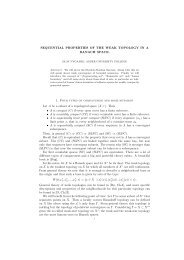
<strong>MAS107</strong> CONTROL THEORY 1. HOVLAND: EXAM SOLUTION 2008 1<br />
<strong>MAS107</strong> <strong>Control</strong> <strong>Theory</strong><br />
<strong>Exam</strong> <strong>Solutions</strong> 2008<br />
Geir Hovland, Mechatronics Group, Grimstad, Norway<br />
June 30, 2008<br />
C. Repeat question 1B, but plot the phase curve instead of the<br />
gain.<br />
I. BODE PLOT<br />
A. Write down the zeroes and poles of the following transfer<br />
function<br />
0.1s<br />
G(s) =<br />
(1 + s<br />
10<br />
)(1 + s<br />
2 10<br />
) 3<br />
This transfer function consists of four parts<br />
• The gain constant 0.1<br />
• The derivator s, which is equal to a zero at location s = 0<br />
• The pole (1 + s<br />
10<br />
), which is equal to a pole at s =<br />
2<br />
−10 2 = −100<br />
• The pole (1 + s<br />
10<br />
), which is equal to a pole at s =<br />
3<br />
−10 3 = −1000<br />
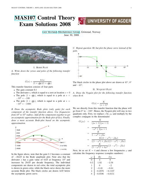
B. Draw the asymptotic Bode plots (only gain) for each<br />
component of the transfer function above. Use frequencies<br />
from 10 0 to 10 5 rad/sec. Add all the components together to get<br />
an asymptotic approximation for the Bode plot of G(s). Finally,<br />
draw a more accurate Bode-plot based on the asymptotic<br />
approximation.<br />
In the figure above, note that the gain 0.1 becomes a constant<br />
of −20dB in the Bode amplitude plot. Note also that the<br />
derivator s has a gain value of 0dB at frequency 10 0 and<br />
increases by 20dB per decade frequency. The individual<br />
components are drawn in red color, the total asymptotic plot<br />
is shown in green color, while the black curve shows the more<br />
accurate Bode plot. The black circles are drawn 3dB below<br />
the asymptotic green curve.<br />
The black circles in the phase plot above are drawn at 45 o , 0 o<br />
and −45 o .<br />
II. NYQUIST PLOT<br />
A. Draw the Nyquist plot for the following transfer function<br />
when K=4.<br />
K<br />
G(s) =<br />
(s + 1) 2<br />
We see directly from this transfer function that the phase will<br />
go from 0 o to −180 o . Hence, the Nyquist plot will stay in two<br />
quadrants only. First, we replace s by jω and multiply by the<br />
complex conjugate in the denominator<br />
G(jω) =<br />
K<br />
(jω + 1)(jω + 1)<br />
=<br />
K<br />
−ω 2 + 2jω + 1<br />
=<br />
K<br />
1 − ω 2 + j2ω<br />
=<br />
K((1 − ω 2 ) − j2ω)<br />
((1 − ω 2 ) + j2ω)((1 − ω 2 ) − j2ω)<br />
=<br />
K<br />
(1 − ω 2 ) 2 + 4ω 2 ((1 − ω2 ) − j2ω)<br />
Next, let us set K = 4 and choose a few frequencies ω and<br />
calculate the frequency response (complex numbers)<br />
ω Re Im<br />
0 4 0<br />
0.5 1.92 −2.56<br />
1 0 −2<br />
2 −0.48 −0.64<br />
4 −0.2076 −0.1107<br />
8 −0.0596 −0.0151
<strong>MAS107</strong> CONTROL THEORY 1. HOVLAND: EXAM SOLUTION 2008 2<br />
This gives us approximately the following Nyquist plot, where<br />
the red curve is from the table above, while the green curve<br />
is the mirror of the red curve about the real axis.<br />
D. Based on the Nyquist plot from question 2A, estimate the<br />
phase margin graphically (no calculations required).<br />
B. Calculate amplitude and phase for the system in question<br />
2A at the following frequencies: 0.5, 1, 2 and 4 rad/sec.<br />
The amplitude A in decibel and phase P are given by the<br />
following formulas.<br />
(√ )<br />
A = 20log 10 Re(G(jω))2 + Im(G(jω)) 2<br />
( )<br />
Im(G(jω))<br />
P = atan<br />
Re(G(jω))<br />
We then get the following results<br />
ω Re Im A P<br />
0.5 1.92 −2.56 10.1 −53.1 o<br />
1 0 −2 6.02 −90 o<br />
2 −0.48 −0.64 −1.94 −126.9 o<br />
4 −0.2076 −0.1107 −12.6 −151.9 o<br />
C. Is the system in question 2A stable for a unity-feedback<br />
controller ?<br />
Yes, the system is stable because N = 0 (the number of<br />
encirclements of -1) and P = 0 (the number of open-loop<br />
unstable poles). The Nyquist criterion says Z = P − N = 0,<br />
which is stable when Z = 0.<br />
A unit circle is drawn in the Nyquist plot, see the figure<br />
above. The phase margin is given by the angle between the<br />
negative real axis and the cross-point between the unit circle<br />
and the Nyquist curve. From the figure this seems to occur<br />
approximately at the black dot representing the frequency<br />
ω = 2. However, the table in question 2B says that the<br />
amplitude A = −1.92dB at ω = 2. Hence, the Nyquist curve<br />
will cross the unit circle slightly before ω = 2 (remember that<br />
an amplitude of 0dB represents the unit circle). The phase<br />
margin at ω = 2 equals 180 o − 126.9 o = 53.1 o . Since the<br />
cross-point occurs slightly before ω = 2, the phase margin is<br />
estimated to be approximately 60 o .<br />
III. TIME AND FREQUENCY RESPONSE<br />
Given the control system in the figure below with the<br />
following plant model:<br />
K<br />
G(s) =<br />
s(s + √ 2K)<br />
A. Describe a method to analytically calculate percentage<br />
overshoot and settling time when a unit step is applied to<br />
the reference input R(s). Hint: Open/closed transfer functions.<br />
First, the closed-loop transfer function is calculated.<br />
G(s)<br />
1 + G(s)<br />
=<br />
=<br />
=<br />
K<br />
s(s+ √ 2K)<br />
K<br />
1 +<br />
s(s+ √ 2K)<br />
K<br />
s 2 + √ 2Ks + K<br />
ω 2<br />
s 2 + 2ζωs + ω 2
<strong>MAS107</strong> CONTROL THEORY 1. HOVLAND: EXAM SOLUTION 2008 3<br />
From the equations above we see that the natural frequency ω<br />
and the damping factor ζ equal<br />
ω = √ √<br />
K<br />
√<br />
2K 2<br />
ζ =<br />
2ω = 2 = 0.707<br />
From the exam formula sheet, we then have the following<br />
relationships between percentage overshoot and settling time.<br />
√<br />
ζ 2 π 2<br />
%OS = 100/exp<br />
T s = 4<br />
ζω = 5.66 √<br />
K<br />
1−ζ 2 = 4.32<br />
B. When a settling time less than 1.0 second is required,<br />
calculate the range of values for the parameter K.<br />
T s = 4<br />
ζω = 5.66 √<br />
K<br />
( ) 2 5.66<br />
K =<br />
= 32<br />
T s<br />
Hence, K must be equal to 32 or larger to achieve a settling<br />
time of 1.0 seconds or less.<br />
C. When a peak time less than 0.2 second is required, calculate<br />
the range of values for the parameter K.<br />
The formula for peak time was specified as follows.<br />
T p =<br />
K =<br />
π<br />
ω √ 1 − ζ = 4.44 √ 2 K<br />
( ) 2 4.44<br />
= 492.8 (1)<br />
T p<br />
Hence, K must be equal to 492.8 or larger to achieve a peak<br />
time of 0.2 seconds or less.<br />
as there is a steady-state control error. Hence, this type of<br />
controller is typically used to achieve zero steady-state error<br />
for Type 0 systems when a step is applied as the reference<br />
input. The integral action appears at low frequencies in the<br />
Bode plot, and hence the PI-controller can be tuned such that<br />
it does not worsen bandwidth performance or stability margins.<br />
PID-<strong>Control</strong>ler: The PID-controller is the same as the PIcontroller<br />
with an added parameter T d which is the derivative<br />
time constant. The derivative action reacts on changes in the<br />
control error. Hence, the derivative action prevents the system<br />
response to change too rapidly. A mechanical equivalent of the<br />
derivative action is a damper mechanism. In the Bode plot, the<br />
derivative action increases both the amplitude and the phase.<br />
Hence, the derivative action can be used to improve system<br />
bandwidth as well as stability margins.<br />
Lag-Compensator: The lag compensator is very similar to<br />
the PI-controller. The main difference is the low frequency<br />
characteristics. While the PI-controller goes to infinity gain<br />
at low frequencies, the lag compensator has a limited gain<br />
at low frequencies. Hence, the lag compensator can reduce<br />
steady-state errors, but not completely remove them.<br />
Lead-Compensator: The lead compensator is very similar<br />
to a PD controller. The main difference is the high frequency<br />
characteristics. While the PD controller goes to infinity gain<br />
at high frequencies, the lead compensator has a limited gain<br />
at high frequencies. This limited gain is a benefit in systems<br />
which contain high frequency measurement noise.<br />
B. The Nyquist curve for a system crosses the real axis at -2,<br />
circles the point -1 once and the system is stable in closed<br />
loop. How many poles in the right half plane does the system<br />
have? Explain your answer.<br />
IV. SYSTEM UNDERSTANDING<br />
A. Explain the properties of the following controllers: P, PI,<br />
PID, lag and lead compensator. Write maximum one page.<br />
P-<strong>Control</strong>ler: The P-controller is the simplest controller<br />
and contains a single parameter usually denoted K p . This<br />
parameter affects only the gain of the system, while the total<br />
phase is unaffected. Hence, a typical method to tune this<br />
controller is to find the frequency ω c where the desired phase<br />
margin in the phase plot occurs, and then adjust the gain<br />
parameter K p such that the amplitude curve crosses the 0dB<br />
line at the same frequency ω c . Systems which are open-loop<br />
stable (no poles in the right half-plane) have an upper limit on<br />
the gain parameter K p for stability, while systems which are<br />
open-loop unstable have a lower limit on the gain parameter.<br />
The P-controller can typically improve system properties such<br />
as rise time, settling time, peak time and steady-state error.<br />
These improvements usually result in a worse performance in<br />
terms of percentage overshoot (stability margin).<br />
PI-<strong>Control</strong>ler: The PI-controller is the same as the P-<br />
controller with an added parameter T i which is the integral<br />
time constant. The integral action will never settle as long<br />
Let us use the Nyquist curve above as a concrete example for<br />
this problem. The Nyquist curve above is a perfect circle with<br />
a radius of 2 and is generated by the following system<br />
G(s) =<br />
2(s + 1)<br />
s − 1
<strong>MAS107</strong> CONTROL THEORY 1. HOVLAND: EXAM SOLUTION 2008 4<br />
The Nyquist curve crosses the real axis at -2, the curve circles C. Design a lag compensator for the system such that the<br />
the point -1 once. The problem text states that the system is steady-state error for a ramp is reduced by a factor of 10<br />
stable in closed-loop. Hence, Z = P − N = 0. Since N = 1, without influencing the system’s bandwidth to a large degree.<br />
we need also that P = 1. In other words, the open-loop system The Bode plot of the open-loop transfer function is given<br />
has one pole in the right half-plane. We can also see that the below.<br />
example transfer function above also has a single pole in the<br />
right half-plane (at s = 1).<br />
C. For the system in question 4B two different P-controllers<br />
are applied. The first P-controller has a gain of 2.0, while the<br />
other controller has a gain of 0.4. Are the two new control<br />
systems stable or unstable. Explain your answers.<br />
The first P-controller will double the radius of the example<br />
circle to 4. The Nyquist curve will still encircle the point<br />
−1 once. Hence, the control system will be stable. The P-<br />
controller with gain 0.4 will change the radius of the example<br />
circle to 0.8. The Nyquist curve will no longer encircle the<br />
point −1. Hence, the P-controller with a gain of 0.4 will be<br />
unstable for this system. Note, that this system behavior is the<br />
opposite of what we see for an open-loop stable system. For<br />
an open-loop unstable system, a large P-controller gain will<br />
First, we multiply the system with the gain of 10. From the<br />
stabilize the system, while small P-controller gains will reduce<br />
Bode plot we see that the cross-over frequency w c = 10 −1 =<br />
the stability margins.<br />
0.1. Hence, to make sure that we do not influence the system<br />
V. STEADY-STATE ERRORS AND COMPENSATOR bandwidth to a large degree, we choose the zero of the lag<br />
compensator equal to 0.01, ie. 1 T<br />
= 0.01 or T = 100. The high<br />
frequency gain of the lag compensator needs to compensate for<br />
1<br />
the initial multiplication of 10. Hence, α = 10, or<br />
αT = 0.001.<br />
The lag compensator and the initial gain of 10 are summarized<br />
as follows and illustrated in the figure below. Note from the<br />
figure that the net gain of the lag compensator and the gain<br />
G p (s) = 0.2<br />
of 10 equals 0dB at high frequencies. This is an important<br />
characteristic too avoid affecting the overall system bandwidth<br />
s(s + 2)<br />
as specified in the problem definition.<br />
The controller equals G c = 10.<br />
A. Calculate the steady-state error when applying a unity step<br />
G c (s) = 10 s + 1 T<br />
α s + 1<br />
αT<br />
at the input R(s).<br />
The system above is a Type 1 system (because of the<br />
= s + 0.01<br />
s + 0.001<br />
integrator). Hence, the steady-state error for a unity step is<br />
equal to 0.<br />
B. Calculate the steady-state error when applying a ramp at<br />
the input R(s).<br />
The control error equals<br />
1<br />
e(s) =<br />
1 + G c (s)G p (s) = 1<br />
1 + 2<br />
s(s+2)<br />
s(s + 2)<br />
=<br />
s(s + 2) + 2<br />
Now we can use the final value theorem to determine the D. Keep the lag compensator from question 5C and add a<br />
steady-state error (knowing that the Laplace transform of a lead compensator such that the bandwidth is increased by a<br />
ramp equals 1 s<br />
). 2 factor 3.<br />
[ ]<br />
1<br />
lim<br />
s→0 s 2 · s · s(s + 2)<br />
We want to increase the cross-over frequency from ω<br />
s(s + 2) + 2<br />
c = 0.1<br />
[<br />
]<br />
s + 2<br />
lim<br />
= 2 to ω c = 0.3. From the Bode plot in Question 5C, we see<br />
s→0 s(s + 2) + 2 2 = 1 that the amplitude at ω c = 0.3 equals approximately −10dB.<br />
Hence, the lead compensator must contribute with a gain of
<strong>MAS107</strong> CONTROL THEORY 1. HOVLAND: EXAM SOLUTION 2008 5<br />
10dB (or 3.16) at ω c . From the formula sheet, we have<br />
|G c (jω c )| =<br />
β =<br />
1<br />
√ β<br />
= 3.16<br />
( ) 2 1<br />
= 0.1<br />
3.16<br />
The formula sheet gives us the final parameter T of the lead<br />
compensator.<br />
ω c =<br />
T =<br />
G c (s) = 1 β<br />
1<br />
T √ β<br />
1 1<br />
√ =<br />
ω c β 0.3 · 0.01 = 10.54<br />
s + 1 T<br />
s + 1<br />
βT<br />
=<br />
10(s + 0.095)<br />
s + 0.95<br />
From the Bode plots below, we see that the lead compensator<br />
raises the gain with 10dB at ω c = 0.3 and that the phase has<br />
its maximum phase lift at the same frequency.<br />
Taking the Laplace transform and inserting m = 1, d = 1, we<br />
can find the transfer function from f(t) to x(t).<br />
x(s 2 + s) = f(s)<br />
x<br />
f (s) = 1<br />
s 2 + 2<br />
B. Calculate the transfer function from the battery voltage to<br />
the current in the figure below.<br />
V (t) = Ri(t) + 1 C<br />
∫<br />
i(t)dt<br />
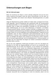
VI. MODELLING<br />
A. Calculate the transfer function from the force f(t) to the<br />
position x(t) for the mechanical system in the figure below.<br />
Taking Laplace, we get the following transfer function<br />
The spring has no effect, since the force f(t) is the same on<br />
both sides of the spring (Newton’s 1st law). The differential<br />
equation which describes the motion of the mass are given<br />
below.<br />
mẍ(t) = f(t) − dẋ(t)<br />
(2)<br />
V (s) = Ri(s) + 1<br />
Cs i(s)<br />
(<br />
= i(s) R + 1 )<br />
Cs<br />
= i(s) RCs + 1<br />
Cs<br />
i<br />
V (s) = Cs<br />
RCs + 1 = 0.5s<br />
0.5s + 1
<strong>MAS107</strong> CONTROL THEORY 1. HOVLAND: EXAM SOLUTION 2008 6<br />
C. The figure below shows two watertanks. The height in tank<br />
1 is h 1 (metre) while the height in tank 2 is h 2 . The area of<br />
tank 1 and 2 are A 1 and A 2 (m 2 ), respectively. The inflow to<br />
tank 1 is u (m 3 /sec) while the outflow is k 1 h 1 . The inflow to<br />
tank 2 is k 1 h 1 , while the outflow is k 2 h 2 . Write down the two<br />
differential equations which describe the system. Based on the<br />
differential equations, write down the transfer function from<br />
u(s) to h2(s).<br />
A 1<br />
h 1<br />
dt<br />
h 2<br />
A 2<br />
dt<br />
Taking Laplace, we get<br />
= u − k 1 h 1<br />
= k 1 h 1 − k 2 h 2<br />
A 1 sh 1 = u − k 1 h 1<br />
h 1 (A 1 s + k 1 ) = u<br />
h 1 =<br />
1<br />
u<br />
A 1 s + k 1<br />
A 2 sh 2 = k 1 h 1 − k 2 h 2<br />
k 1<br />
h 2 (A 2 s + k 2 ) = k 1 h 1 = u<br />
(<br />
A 1 s<br />
)<br />
+<br />
(<br />
k 1<br />
)<br />
h 2<br />
u (s) = 1<br />
k 1<br />
A 2 s + k 2 A 1 s + k 1