Universität Karlsruhe (TH) - am Institut für Baustatik

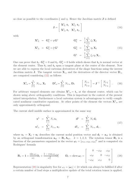
as close as possible to the coordinates ξ and η. Hence the Jacobian matrix J is defined
with
⎡
J = ⎣ Xh , ξ ·t 1 X h ⎤
, ξ ·t 2
⎦ (14)
X h , η ·t 1 X h , η ·t 2
X h , ξ = G 0 ξ + η G 1 G 0 ξ = 1 4∑
ξ I X I
4
I=1
X h , η = G 0 η + ξ G 1 G 0 η = 1 4∑
η I X I
4
I=1
G 1 = 1 4∑
ξ I η I X I .
4
I=1
One can prove that t 3 · G 0 ξ =0andt 3 · G 0 η = 0 holds which shows that t 3 is normal vector at
the element center. Thus t 1 and t 2 span a tangent plane at the center of the element. Now
we are able to express the local cartesian derivatives of the shape functions using the inverse
Jacobian matrix J. The tangent vectors X, α and the derivatives of the director vector D, α
are computed considering (12) as follows
X h , α =
4∑
I=1
N I , α X I D h , α =
4∑
I=1
(15)
[ ] [ ]
NI ,
N I , α D 1
I = J −1 NI , ξ
. (16)
N I , 2 N I , η
For arbitrary warped elements one obtains X h , α = t α at the element center, which can be
shown using above orthogonality conditions. This is important in the context of the present
mixed interpolation. Furthermore a local cartesian system is advantageous to verify complicated
nonlinear constitutive equations. At other points of the element the vectors X h , α are
only approximately orthogonal.
The current shell middle surface is approximated in the same way
x h =
x h , α =
4∑
N I x I d h =
I=1
4∑
N I , α x I d h , α =
I=1
4∑
N I d I
I=1
4∑
N I , α d I ,
I=1
(17)
where x I = X I + u I describes the current nodal position vector and d I = a 3I is obtained
by an orthogonal transformation a kI = R I A kI , k =1, 2, 3. The rotation tensor R I is a
function of the parameters organized in the vector ω I =[ω 1I ,ω 2I ,ω 3I ] T and is computed via
Rodrigues’ formula
R I = 1 + sin ω I
ω I
Ω I + 1 − cos ω I
Ω 2
ωI
2 I Ω I =skewω I =
⎡
⎤
0 −ω 3I ω 2I
ω
⎢ 3I 0 −ω 1I
⎥
⎣
⎦
−ω 2I ω 1I 0
Representation (18) is singularity free for ω I = |ω I | < 2π which can always be fulfilled if after
a certain number of load steps a multiplicative update of the total rotation tensor is applied.
7
(18)