Universität Karlsruhe (TH) - am Institut für Baustatik
Universität Karlsruhe (TH) - am Institut für Baustatik
Universität Karlsruhe (TH) - am Institut für Baustatik

Create successful ePaper yourself
Turn your PDF publications into a flip-book with our unique Google optimized e-Paper software.
B<br />
Remarks on patch test and stability<br />
Assuming infinitesimal deformations δv e e =1, 2..., numel we ex<strong>am</strong>ine conditions to fulfil the<br />
patch test and stability conditions for the discrete problem based on the presented mixed<br />
formulation. The described FE–method can be interpreted as a ¯B − approach.<br />
B.1 The patch test<br />
Introduce<br />
¯B := N ε F T −1 G (50)<br />
the material part of the element stiffness matrix can be reformulated as follows<br />
∫<br />
k m = G T ĤG= ¯B T C ¯B dA . (51)<br />
Now consider an element displacement vector δv, such that<br />
B δv ≡ constant (52)<br />
(Ω e)<br />
for each element and formulate<br />
⎡ ∫<br />
¯B δv = N ε F T −1 G δv = [ ] ⎡<br />
1, Ñε ⎣ 1/A ⎤<br />
e 1 0<br />
0 f T −1 ⎦<br />
⎢<br />
⎣<br />
(Ω e)<br />
∫<br />
(Ω e)<br />
B δv dA<br />
Ñ T σ B δv dA<br />
⎤<br />
⎥<br />
⎦<br />
(53)<br />
which yields<br />
¯B δv = ε 0 ≡ constant (54)<br />
if the following two conditions hold:<br />
1<br />
(i) (Ω B δv dA = B(ξ = η =0)δv = e) ε0 . This is fulfilled for the shear part with<br />
assumed strains, but not with the standard bilinear finite element interpolation of the<br />
displacement field along with (5) 3 . In this context we refer to the investigations for a<br />
linear plate [33].<br />
A e<br />
∫<br />
(ii) ∫ (Ω e) ÑT σ dA = 0 , which is the case for the present interpolation.<br />
Thus ε 0 ≡ constant yields with C = constant for an arbitrary patch of elements to a constant<br />
stress state.<br />
B.2 Stability of the discrete problem<br />
Here the numerical stability of the presented mixed hybrid shell element with 20 nodal degrees<br />
of freedom based on the Hu–Washizu functional is discussed. We assume that C is positive<br />
definite and that the geometric contribution to the tangential stiffness does not introduce<br />
instabilities. We denote by ker[B] the null space of B. Recall that ker[B] consists all nodal<br />
infinitesimal rigid body motions, i.e. a vector δv R in ker[B] satisfies<br />
B δv R = 0 ⇔ δv R = nodal rigid body motion (55)<br />
25