Universität Karlsruhe (TH) - am Institut für Baustatik
Universität Karlsruhe (TH) - am Institut für Baustatik Universität Karlsruhe (TH) - am Institut für Baustatik
esultants σ is approximated as follows σ h = N σ ˆσ N σ = [1 8 , Ñσ] Ñ σ = N m σ = ⎡ ⎢ ⎣ N m σ 0 0 0 N b σ 0 0 0 N s σ ⎡ J11J 0 11(η 0 − ¯η) ⎢ ⎣ J12J 0 12(η 0 − ¯η) J11J 0 12(η 0 − ¯η) ⎤ ⎥ ⎦ N m σ = N b σ J21J 0 21(ξ 0 − ¯ξ) ⎤ J22J 0 22(ξ 0 − ¯ξ) ⎥ J21J 0 22(ξ 0 − ¯ξ) ⎦ N s σ = [ J 0 11 (η − ¯η) J21(ξ 0 − ¯ξ) ] J12(η 0 − ¯η) J22(ξ 0 − ¯ξ) Here, we denote by 1 8 an eight order unit matrix. The vector ˆσ contains 8 parameters for the constant part and 6 parameters for the varying part of the stress field, respectively. The interpolation of the membrane forces and bending moments corresponds to the procedure in [31], see also the original approach for plane stress problems with ¯ξ =¯η =0in[32]. The transformation coefficients Jαβ 0 = J αβ (ξ =0,η = 0) are the components of the Jacobian matrix J (14) evaluated at the element center. Due to the constants ¯ξ = 1 ∫ ξdA ¯η = 1 ∫ ∫ ηdA A e = A e A e dA (39) (Ω e) the linear functions are orthogonal to the constant function which yields partly decoupled matrices. In this context we refer also to [33] in the case of a plate formulation. The independent shell strains are approximated with 14 parameters in ˆε ε h = N ε ˆε N ε = [1 8 , Ñε] Ñ ε = N m ε = ⎡ ⎢ ⎣ N m ε 0 0 0 N b ε 0 0 0 N s ε ⎡ J11J 0 11(η 0 − ¯η) ⎢ ⎣ J12J 0 12(η 0 − ¯η) 2J11J 0 12(η 0 − ¯η) ⎤ (Ω e) (Ω e) ⎥ ⎦ N m ε = N b ε J21J 0 21(ξ 0 − ¯ξ) ⎤ J22J 0 22(ξ 0 − ¯ξ) ⎥ 2J21J 0 22(ξ 0 − ¯ξ) ⎦ N s ε = N s σ . Thus, the independent stresses and strains are interpolated with the same shape functions. We remark that (38) and(40) contain a transformation of the contravariant tensor components to the local cartesian coordinate system at the element center. 3.5 Linearized variational formulation Inserting above interpolations for the displacements, stresses and strains into the linearized stationary condition yields L [g(θ h ,δθ h ), Δθ h ]:=g(θ h ,δθ h )+Dg · Δθ h = numel ∑ e=1 ⎡ ⎢ ⎣ δv δˆε δ ˆσ ⎤T ⎧⎡ ⎪⎨ ⎥ ⎢ ⎦ ⎣ ⎪⎩ e k g 0 G T 0 H −F G −F T 0 12 ⎤ ⎡ ⎥ ⎦ ⎢ ⎣ Δv Δˆε Δˆσ ⎤ ⎥ ⎦ + ⎡ ⎢ ⎣ f i − f a f e f s ⎤⎫ ⎪⎬ ⎥ ⎦ ⎪⎭ e (38) (40) (41)
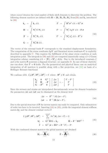
where numel denotes the total number of finite shell elements to discretize the problem. The following element matrices are defined with B =[B 1 , B 2 , B 3 , B 4 ] from(29) andk σ introduced in (36) ∫ ∫ k g = k σ dA f i = B T σ h dA = G T ˆσ Ω e Ω e ∫ ∫ H = N T ε CN ε dA f e = N T ε ∂εW dA− F ˆσ Ω e Ω e ∫ ∫ (42) F = N T ε N σ dA f s = N T σ ε h G dA − F T ˆε Ω e Ω e ∫ G = N T σ B dA . Ω e The vector of the external loads f a corresponds to the standard displacement formulation. The computation of the stress resultants ∂εW and linearized stress resultants C is explicitly described in appendix C. This requires the fulfillment of the plane stress condition at each integration point. The integrals in (39)and(42) are computed numerically using a 2×2Gauss integration scheme considering dA = |X h , ξ ×X h , η | dξdη. Due to the introduced constants ¯ξ and ¯η the matrix F possesses a diagonal structure, see appendix D. In case of linear elasticity one can show, that f e ≡ 0 holds. For the geometrical and physical linear case an analytical integration of all matrices is possible along with a flat projection, see [34] on basis of a Hellinger–Reissner functional. We continue with L[g(θ h ,δθ h ), Δθ h ]=0 where δθ h ≠ 0 and obtain ⎡ ⎢ ⎣ k g 0 G T 0 H −F G −F T 0 ⎤ ⎡ ⎥ ⎦ ⎢ ⎣ Δv Δˆε Δˆσ ⎤ ⎡ ⎥ ⎢ ⎦ = − ⎣ f i − f a f e f s ⎤ ⎥ ⎦ (43) Since the stresses and strains are interpolated discontinuously across the element boundaries the parameters Δˆε and Δˆσ can be eliminated on the element level Δˆε = F T −1 (G Δv + f s ) Δˆσ = F −1 (H Δˆε + f e ) . (44) Due to the special structure of F the inverse matrix can easily be computed. Only submatrices of order two have to be inverted. Inserting (44) in(43) 1 yields the tangential element stiffness matrix k e T and the element residual vector ˆf L [g(θ h ,δθ h ), Δθ h ] = numel ∑ e=1 δv T (k e T Δv + ˆf) =0 k e T = G T ĤG+ k g Ĥ = F −1 HF T −1 ˆf = G T (ˆσ + Ĥfs + F −1 f e ) − f a (45) With the condensed element matrices the global matrices are obtained numel numelˆf . (46) K T = A e=1 k e T ˆF = A e=1 13
- Page 1 and 2: Universität Karlsruhe (TH) Institu
- Page 3 and 4: A robust nonlinear mixed hybrid qua
- Page 5 and 6: the strain field and the non-consta
- Page 7 and 8: with membrane strains ε αβ , cur
- Page 9 and 10: as close as possible to the coordin
- Page 11 and 12: with δγξ M = [δx, ξ ·d + x,
- Page 13: To avoid numerical difficulties the
- Page 17 and 18: 4 Examples The derived element form
- Page 19 and 20: 4.3 Hemispherical shell with a 18
- Page 21 and 22: Load P [N] 3,5 3,0 2,5 2,0 1,5 1,0
- Page 23 and 24: Load P in kN 20,0 18,0 16,0 14,0 12
- Page 25 and 26: 200 175 150 Load P [kN] 125 100 u_z
- Page 27 and 28: B Remarks on patch test and stabili
- Page 29 and 30: The plane stress condition S 33 (E
- Page 31 and 32: E J 2 -plasticity model for small s
- Page 33 and 34: [16] Betsch P, Gruttmann F, Stein,
where numel denotes the total number of finite shell elements to discretize the problem. The<br />
following element matrices are defined with B =[B 1 , B 2 , B 3 , B 4 ] from(29) andk σ introduced<br />
in (36)<br />
∫<br />
∫<br />
k g = k σ dA f i = B T σ h dA = G T ˆσ<br />
Ω e Ω e<br />
∫<br />
∫<br />
H = N T ε CN ε dA f e = N T ε ∂εW dA− F ˆσ<br />
Ω e Ω e<br />
∫<br />
∫<br />
(42)<br />
F = N T ε N σ dA f s = N T σ ε h G dA − F T ˆε<br />
Ω e Ω e<br />
∫<br />
G = N T σ B dA .<br />
Ω e<br />
The vector of the external loads f a corresponds to the standard displacement formulation.<br />
The computation of the stress resultants ∂εW and linearized stress resultants C is explicitly<br />
described in appendix C. This requires the fulfillment of the plane stress condition at each<br />
integration point. The integrals in (39)and(42) are computed numerically using a 2×2Gauss<br />
integration scheme considering dA = |X h , ξ ×X h , η | dξdη. Due to the introduced constants ¯ξ<br />
and ¯η the matrix F possesses a diagonal structure, see appendix D. In case of linear elasticity<br />
one can show, that f e ≡ 0 holds. For the geometrical and physical linear case an analytical<br />
integration of all matrices is possible along with a flat projection, see [34] on basis of a<br />
Hellinger–Reissner functional.<br />
We continue with L[g(θ h ,δθ h ), Δθ h ]=0 where δθ h ≠ 0 and obtain<br />
⎡<br />
⎢<br />
⎣<br />
k g 0 G T<br />
0 H −F<br />
G −F T 0<br />
⎤ ⎡<br />
⎥<br />
⎦<br />
⎢<br />
⎣<br />
Δv<br />
Δˆε<br />
Δˆσ<br />
⎤ ⎡<br />
⎥ ⎢<br />
⎦ = − ⎣<br />
f i − f a<br />
f e<br />
f s<br />
⎤<br />
⎥<br />
⎦ (43)<br />
Since the stresses and strains are interpolated discontinuously across the element boundaries<br />
the par<strong>am</strong>eters Δˆε and Δˆσ can be eliminated on the element level<br />
Δˆε = F T −1 (G Δv + f s )<br />
Δˆσ = F −1 (H Δˆε + f e ) .<br />
(44)<br />
Due to the special structure of F the inverse matrix can easily be computed. Only submatrices<br />
of order two have to be inverted. Inserting (44) in(43) 1 yields the tangential element stiffness<br />
matrix k e T and the element residual vector ˆf<br />
L [g(θ h ,δθ h ), Δθ h ] =<br />
numel ∑<br />
e=1<br />
δv T (k e T Δv + ˆf) =0<br />
k e T = G T ĤG+ k g Ĥ = F −1 HF T −1<br />
ˆf = G T (ˆσ + Ĥfs + F −1 f e ) − f a (45)<br />
With the condensed element matrices the global matrices are obtained<br />
numel<br />
numelˆf . (46)<br />
K T = A<br />
e=1<br />
k e T<br />
ˆF = A<br />
e=1<br />
13


