Universität Karlsruhe (TH) - am Institut für Baustatik
Universität Karlsruhe (TH) - am Institut für Baustatik
Universität Karlsruhe (TH) - am Institut für Baustatik

Create successful ePaper yourself
Turn your PDF publications into a flip-book with our unique Google optimized e-Paper software.
esultants σ is approximated as follows<br />
σ h = N σ ˆσ N σ = [1 8 , Ñσ]<br />
Ñ σ =<br />
N m σ =<br />
⎡<br />
⎢<br />
⎣<br />
N m σ 0 0<br />
0 N b σ 0<br />
0 0 N s σ<br />
⎡<br />
J11J 0 11(η 0 − ¯η)<br />
⎢<br />
⎣ J12J 0 12(η 0 − ¯η)<br />
J11J 0 12(η 0 − ¯η)<br />
⎤<br />
⎥<br />
⎦ N m σ = N b σ<br />
J21J 0 21(ξ 0 − ¯ξ) ⎤<br />
J22J 0 22(ξ 0 − ¯ξ) ⎥<br />
J21J 0 22(ξ 0 − ¯ξ)<br />
⎦ N s σ =<br />
[<br />
J<br />
0<br />
11 (η − ¯η) J21(ξ 0 − ¯ξ)<br />
]<br />
J12(η 0 − ¯η) J22(ξ 0 − ¯ξ)<br />
Here, we denote by 1 8 an eight order unit matrix. The vector ˆσ contains 8 par<strong>am</strong>eters for<br />
the constant part and 6 par<strong>am</strong>eters for the varying part of the stress field, respectively. The<br />
interpolation of the membrane forces and bending moments corresponds to the procedure in<br />
[31], see also the original approach for plane stress problems with ¯ξ =¯η =0in[32]. The<br />
transformation coefficients Jαβ<br />
0 = J αβ (ξ =0,η = 0) are the components of the Jacobian<br />
matrix J (14) evaluated at the element center. Due to the constants<br />
¯ξ = 1 ∫<br />
ξdA ¯η = 1 ∫<br />
∫<br />
ηdA A e =<br />
A e<br />
A e<br />
dA (39)<br />
(Ω e)<br />
the linear functions are orthogonal to the constant function which yields partly decoupled<br />
matrices. In this context we refer also to [33] in the case of a plate formulation.<br />
The independent shell strains are approximated with 14 par<strong>am</strong>eters in ˆε<br />
ε h = N ε ˆε N ε = [1 8 , Ñε]<br />
Ñ ε =<br />
N m ε =<br />
⎡<br />
⎢<br />
⎣<br />
N m ε 0 0<br />
0 N b ε 0<br />
0 0 N s ε<br />
⎡<br />
J11J 0 11(η 0 − ¯η)<br />
⎢<br />
⎣ J12J 0 12(η 0 − ¯η)<br />
2J11J 0 12(η 0 − ¯η)<br />
⎤<br />
(Ω e)<br />
(Ω e)<br />
⎥<br />
⎦ N m ε = N b ε<br />
J21J 0 21(ξ 0 − ¯ξ) ⎤<br />
J22J 0 22(ξ 0 − ¯ξ) ⎥<br />
2J21J 0 22(ξ 0 − ¯ξ)<br />
⎦ N s ε = N s σ .<br />
Thus, the independent stresses and strains are interpolated with the s<strong>am</strong>e shape functions. We<br />
remark that (38) and(40) contain a transformation of the contravariant tensor components<br />
to the local cartesian coordinate system at the element center.<br />
3.5 Linearized variational formulation<br />
Inserting above interpolations for the displacements, stresses and strains into the linearized<br />
stationary condition yields<br />
L [g(θ h ,δθ h ), Δθ h ]:=g(θ h ,δθ h )+Dg · Δθ h<br />
=<br />
numel ∑<br />
e=1<br />
⎡<br />
⎢<br />
⎣<br />
δv<br />
δˆε<br />
δ ˆσ<br />
⎤T<br />
⎧⎡<br />
⎪⎨<br />
⎥ ⎢<br />
⎦ ⎣<br />
⎪⎩<br />
e<br />
k g 0 G T<br />
0 H −F<br />
G −F T 0<br />
12<br />
⎤ ⎡<br />
⎥<br />
⎦<br />
⎢<br />
⎣<br />
Δv<br />
Δˆε<br />
Δˆσ<br />
⎤<br />
⎥<br />
⎦ +<br />
⎡<br />
⎢<br />
⎣<br />
f i − f a<br />
f e<br />
f s<br />
⎤⎫<br />
⎪⎬<br />
⎥<br />
⎦<br />
⎪⎭<br />
e<br />
(38)<br />
(40)<br />
(41)