Sensors for ecology - Outil de Suivi des Contrats

Présentation de l’éditeur
Ecological sciences deal with the way organisms interact
with one another and their environment. Using sensors
to measure various physical and biological characteristics
has been a common activity since long ago. However
the advent of more accurate technologies and increasing
computing capacities demand a better combination
of information collected by sensors on multiple spatial,
temporal and biological scales.
This book provides an overview of current sensors for
ecology and makes a strong case for deploying integrated
sensor platforms. By covering technological challenges as
well as the variety of practical ecological applications, this text is meant to be
an invaluable resource for students, researchers and engineers in ecological
sciences.
This book benefited from the Centre National de la Recherche Scientifique
(CNRS) funds, and includes 16 contributions by leading experts in french
laboratories.
Key features
• An overview of sensors in the field of animal behaviour and physiology,
biodiversity and ecosystem.
• Several case studies of integrated sensor platforms in terrestrial and aquatic
environments for observational and experimental research.
• Presentation of new applications and challenges in relation with remote
sensing, acoustic sensors, animal-borne sensors, and chemical sensors.

Sensors for ecology
Towards integrated knowledge of ecosystems

Jean-François Le Galliard,
Jean-Marc Guarini, Françoise Gaill
Sensors for ecology
Towards integrated knowledge
of ecosystems
Centre National de la recherche scientifique (CNRS)
Institut Écologie et Environnement (INEE)
www.cnrs.fr

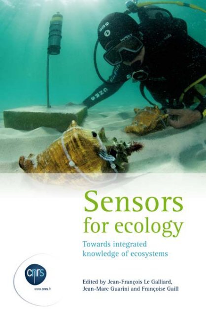
Photographie de couverture / Cover Picture
© CNRS Photothèque – AMICE Erwan
UMR6539 – Laboratoire des sciences de l’environnement marin – LEMAR – PLOUZANE
“A diver inspects a queen conch Strombus gigas during a scientific expedition
in Mexico. The queen conch is equipped with acoustic sensors, here nearby a receptor,
in order to collect information on its behaviour and physiology in nature.”
© CNRS, Paris, 2012
ISBN : 978-2-9541683-0-2

Contents
Foreword................................................................................................ 11
I
Ecophysiology and animal behaviour
Chapter 1 :
Bio-logging: recording the ecophysiology and behaviour of animals
moving freely in their environment
Yan Ropert-Coudert, Akiko Kato, David Grémillet, Francis Crenner.... 17
Chapter 2 :
Animal-borne sensors to study the demography and behaviour
of small species
Olivier Guillaume, Aurélie Coulon, Jean-François Le Galliard,
and Jean Clobert................................................................................... 43
Chapter 3 :
Passive hydro-acoustics for cetacean census and localisation
Flore Samaran, Nadège Gandilhon, Rocio Prieto Gonzalez, Federica
Pace, Amy Kennedy, and Olivier Adam............................................... 63
Chapter 4 :
Bioacoustics approaches to locate and identify animals in terrestrial
environments
Chloé Huetz, Thierry Aubin................................................................. 83

8 Contents
II
Biodiversity
Chapter 1 :
Global estimation of animal diversity using automatic acoustic
sensors
Jérôme Sueur, Amandine Gasc, Philippe Grandcolas, Sandrine Pavoine. 99
Chapter 2 :
Assessing the spatial and temporal distributions of zooplankton
and marine particles using the Underwater Vision Profiler
Lars Stemmann, Marc Picheral, Lionel Guidi, Fabien Lombard,
Franck Prejger, Hervé Claustre, Gabriel Gorsky..................................... 119
Chapter 3 :
Assessment of three genetic methods for a faster and reliable
monitoring of harmful algal blooms
Jahir Orozco-Holguin, Kerstin Töbe, Linda K. Medlin.......................... 139
Chapter 4 :
Automatic particle analysis as sensors for life history studies in
experimental microcosms
François Mallard, Vincent Le Bourlot, Thomas Tully............................ 163
III
Ecosystem properties
Chapter 1 :
In situ chemical sensors for benthic marine ecosystem studies
Nadine Le Bris, Leonardo Contreira-Pereira, Mustafa Yücel................. 185
Chapter 2 :
Advances in marine benthic ecology using in situ chemical sensors
Nadine Le Bris, Leonardo Contreira-Pereira, Mustafa Yücel................. 209
Chapter 3 :
Use of global satellite observations to collect information in marine
ecology
Séverine Alvain, Vincent Vantrepotte, Julia Uitz, Lucile Duforêt-
Gaurier................................................................................................. 227

Contents 9
Chapter 4 :
Tracking canopy phenology and structure using ground-based
remote sensed NDVI measurements
Jean-Yves Pontailler, Kamel Soudani.................................................... 243
IV
Integrated studies
Chapter 1 :
Integrated observation system for pelagic ecosystems and
biogeochemical cycles in the oceans
Lars Stemmann, Hervé Claustre, Fabrizio D’Ortenzio.......................... 261
Chapter 2 :
Tropical rain forest environmental sensors at the Nouragues
experimental station, French Guiana
Jérôme Chave, Philippe Gaucher, Maël Dewynter.................................. 279
Chapter 3 :
Use of sensors in marine mesocosm experiments to study the effect
of environmental changes on planktonic food webs
Behzad Mostajir, Jean Nouguier, Emilie Le Floc’h, Sébastien Mas,
Romain Pete, David Parin, Francesca Vidussi....................................... 305
Synthesis and conclusion
Jean-François Le Galliard, Jean-Marc Guarini and Françoise Gaill...... 331
NB: When cited in the text, a chapter of this book is identified according
to the part it belongs to. For example, (III, 3) refers to the chapter
3 by Alvain et al. in the third (III) part of this book about Ecosystem
properties.

Foreword
Altogether explorer, scientist, philosopher and one of the first world citizen,
the German naturalist Alexander von Humboldt (1769-1859) is often
considered as a founder of ecological sciences, though the word “ecology”
was only coined several decades later by another German scientist, Ernst
Haeckel (1834-1919). Equipped with the best sensors (thermometers,
barometers, and so on) and familiar with advanced metrology techniques
of its time, von Humboldt pioneered the field of plant biogeography, a
discipline at the meeting point between botany, geography, climatology
and geology. Von Humboldt major conceptual and methodological contributions
consisted in collecting physical and geological data along with
plant distribution maps to determine the physical and historical conditions
favouring specific plant assemblages all over the world. With this
approach, he ventured into previously unsuspected complex interactions
between plants and their physical surroundings. Two centuries later,
researchers are still striving to understand the ecological and evolutionary
mechanisms that determine the distribution of plant and animal species.
Indeed, an accurate quantification of how organisms interact with each
other and with their environment is at the heart of several grand challenges
in modern ecological sciences from the description of bio-geochemical
balances to the prediction of ecosystem dynamics. However, contrary
to von Humboldt and his followers, we can now explore thoroughly the
natural world, thanks to major technological improvements in our ability
to measure physical, chemical and biological quantities. Sensors are now
part of the standard toolbox of most ecological studies, and play an important
role in both exploratory studies of nature, experimental approaches,
and the development of predictive ecological models. With the advent
of more advanced technologies and the strong opportunities offered by
nowadays available computing capacities, we are in a better position to
integrate ecological information from sensors across multiple spatial, temporal
and biological scales. This book, sponsored by the Centre National
de la Recherche Scientifique (CNRS) in France, presents an up-to-date
overview of the use sensors for ecology by some leading CNRS laborato-

12 Foreword
ries. The book covers some of the main technological challenges in our
field from bio-loggers attached on animals to remote sensing imaging
capacities installed on satellites, and provides many examples of practical
applications chosen from ongoing CNRS programs. It is also tightly
connected with the current frontiers in ecology and evolution throughout
the world. We hope that the book will become an invaluable resource to
students, researchers and engineers in ecological sciences.
Few books have reviewed methods and issues in the field of sensors for
ecology. The reason is easy to understand: a great deal of techniques
and sensor types do exist and are covered in specific reviews or journals.
Keeping pace with the increasing number of sensors and technologies
currently available is therefore a difficult task. Yet, this book provides
in a synthetic way a balanced description of the new applications and
challenges in ecological research that the use of remote, acoustic, animalborne,
chemical and genosensors represents. Here, we adopted a broad
view on sensors – usually defined as a device that measures a physical
quantity and converts it into a signal – to describe a quantity of tools
including image and video analyses, biodiversity and life history sensors,
and other less traditional methods.
Furthermore, this book contains technical descriptions of some sensors
even though it is not a handbook about sensor technologies. A technical
treatment is crucial to understand, design and integrate sensors for
the purpose of ecological research, but this issue is already addressed in
many handbooks. Instead, it was decided to focus this presentation on
relevant applications and practical problems faced by ecologists during
their research programs.
Lastly, the book differs from a traditional presentation based on a standard
classification among sensor types and a discussion of the specific
issues within each category of sensors (e.g. remote sensing versus chemical
sensors). Ecological studies often need to integrate physical, chemical and
biological data obtained with various types of sensors to get a comprehensive
view of the state and dynamics of ecosystems. We therefore chose to
make a strong case for the deployment of integrated, autonomous sensor
platforms in the context of observational and experimental research infrastructures,
and we present case studies where integrated data can inform
predictive models. The integration of various types of sensors for ecological
studies poses a series of complex problems, from the engineering and
autonomy of the platform to the access and use of data for modelling.
These difficulties go far beyond the design of a single sensor and are often
specific of the scale at which sensors should be deployed.

Foreword 13
The idea of this project started under the patronage of the CNRS Institut
Écologie et Environnement in 2010 with the aim to produce a state-ofthe-art
review for sensors used in ecology in France, as well as to identify
strengths and weaknesses in this field for the future. Under the supervision
of Jean-Marc Guarini and Karine Heerah, a workshop was organised at the
University Pierre and Marie Curie in Paris in January 2011. Twenty four
contributions were made and the workshop’s program addressed remote
sensing techniques, the use of sensors for in situ studies, and the use of
sensors for experimental studies. From these contributions and the discussions
that followed, a few were selected to be published in the four
sections of this book. The first section deals with animal behaviour and
physiology, a very active field of research that raises both strong technical
constraints and ethical issues. In a second section, we discuss the use of
sensors in intra-specific and inter-specific biodiversity studies, and provide
key examples ranging from the use of acoustic sensors or genetic methods
to image analysis. We then present a series of ecosystem studies relying
on advanced remote sensing and chemical sensors; those studies focus
on measuring feedbacks between organisms and their geo-chemical environment.
Our last section groups three integrated ecological studies. Two
discuss observation platforms of ecosystems and one describes an experimental
marine ecology infrastructure. The latter demonstrates how sensors
can be used to manipulate environmental conditions and study the
effect of environmental changes on ecosystems. Each chapter was organised
so that it reviews existing methods and sensors, and discusses current
difficulties and requirements for future technological development.
We would like to thank the authors for their participation and their kind
patience during the editorial process. Angeline Perrot assisted us during
the two last months of this project and was extremely efficient at organising
reviews, editing all text and making the iconography tidy from an
heterogeneous pool of figures and photographs. The editors would like to
thank the CNRS and the Institut Écologie et Environnement (INEE) for
their financial support, as well as the University Pierre and Marie Curie
for hosting the workshop. Jean-François Le Galliard acknowledges the support
of the TGIR Ecotrons program and from the UMS 3194 CEREEP-
Ecotron IleDeFrance as well as the financial support from ANR Equipex
PLANAQUA coordinated by École normale superieure and CNRS (contract
ANR-10-EQPX-13).
Jean-François Le Galliard, Jean-Marc Guarini and Françoise Gaill
January 16, 2012
Paris, France

I
EcoPHySIology
AND ANIMAL bEHAVIoUR

Chapter 1
Bio-logging: recording
the ecophysiology and behaviour
of animals moving freely in their
environment
Yan Ropert-Coudert, Akiko Kato, David Grémillet, Francis Crenner
1. Setting the scene
1.1 Sensing with bio-loggers
Bio-logging refers to the fastening of autonomous devices onto (mainly)
free-ranging animals to collect physical and biological information
(Naito, 2004; 2010; Cooke et al., 2004; Ropert-Coudert et al., 2005; see
also Costa, 1988, although the term bio-logging was not used in these
times). It should be noted here that bio-logging is sometimes referred to
as biologging. However, as Naito (2010) pointed out, the latter term is
misleading as it is used in molecular biology. As such bio-logging differs
from telemetry in the sense that data are stored locally in the memory
of the devices and not transferred via radio waves or other transmitting
means. This move from biotelemetry to bio-logging was done in order
to address practical difficulties related to data transmission. Thus, this
comes, as no surprise that bio-logging was firstly used in ecological and
physiological studies to investigate marine, far-ranging, diving species, as
water represents a barrier to radio signals. Bio-logging studies were initially
conducted on species with a body mass large enough to accommodate the
large size of the very first loggers: seals and whales. As miniaturisation
progressed, smaller species of seals and seabirds became target species for
bio-logging approaches. Among seabirds, penguins (Sphenscidae) represent
an intensively studied family because of their adaptation to aquatic life

18 Ecophysiology and animal behaviour
and their consequently denser, larger and more robust body. Nowadays,
bio-logging can be applied onto an impressive range of species, terrestrial
or aquatic, whether these are mammals, birds or reptiles (see I, 2).
Bio-logging developments are one step away from moving into the insect
realm as radio-telemetry is already available to study terrestrial and flying
insects (Vinatier et al., 2010; Wikelski et al., 2006).
Immediate consequences of local storage are the necessity to retrieve the
device to access the data and develop appropriate sensors to gather data
about physical and biological information on relevant time scales. It therefore
clearly appears that bio-logging primarily refers to a methodological
approach and has generated research to improve existing technologies. Yet,
bio-logging is more than a mere catalogue of tools and techniques. The
possibility to obtain an uninterrupted flow of information pertaining to
both the activity and physiology of animal and its immediate, physical
surroundings revolutionised the way we consider several fields in biology.
We could draw a parallel with the field of genetics and how it evolved from
Gregor Mendel crossing variety of peas to the advanced technologies of
molecular sequencing. Similarly, the ecologist with its notebook possesses
now a suite of approaches to examine animals living freely in their environment.
In this context, bio-logging applications ranges from physiological
investigations to the comprehension of the functioning of ecosystems,
by relating a change in physical parameters of the environment to a change
in the behaviour of both a predator and its prey, at the same spatial and
temporal scales (Ropert-Coudert et al., 2009a).
1.2. Bio-logging in the scientific community
The word bio-logging was coined at the occasion of the first symposium
about the topic held in 2003 in Tokyo, Japan. Over the past decade, three
additional symposia took place: Saint Andrews (Scotland) in 2005, Pacific
Grove (USA) in 2008, and Hobart (Tasmania) in 2011. The next bio-logging
symposium will be organized in France and is tentatively scheduled
for Strasbourg in September 2014. The number of manufacturers has
steadily increased since the inception of Wildlife Computers (USA) in
1986, the first – to the best of our knowledge – bio-logging company ever.
Nowadays, the core of the bio-logging production is concentrated in the
North America and Japan (Ropert-Coudert et al., 2009b), but emerging
companies in the UK (CTL), Iceland (Star-Oddi) or Italy (Technosmart)
are gaining worldwide momentum (Table 1). A non-negligible proportion
(a rough estimate of 20%) of bio-logging devices is still produced in
research institutions, the so-called custom-made bio-loggers, and is thus
accessible only through collaborations between researchers. In Europe,
for example, research-driven developments are found in the Sea Mammal

Part I – Chapter 1 19
Table 1: A non exhaustive list of the most-used bio-loggers together
with their weights and the sensors they include, as well as the name
of the manufacturers.
Model Weight (g) Sensors Manufacturers
Mk 15 2.5 Light, wet or dry status British Antarctic Survey, UK
Cefas G5 2.7 Depth, temperature Cefas technology Ltd, UK
DST bird 1.7 Temperature, light
Star-Oddi, Iceland
DST magnetic 19 Depth, temperature, magnetometer, tilt
ORI400-D3GT 9 Depth, temperature, acceleration
W1000-3MPD3GT 130 Depth, temperature, speed, acceleration, magnetometer
Little Leonardo, Japan
W400-ECG 57 ECG
DSL400-VDT II 82 Depth, temperature, image
GiPSy I 22 GPS TechnoSmart, Italy
CatTraQ 22 GPS Mr. Lee, USA
Mk9 30 Depth, temperature, light, acceleration, magnetometer
Wildlife Computers, USA
SPLASH10-F-400 225 Depth, temperature, light, GPS, Argos (data transmission)
DTAG 300 Depth, audio, pitch, roll, heading
SRDL tag 370 Depth, temperature, speed, Argos (data transmission)
CTD tag 545 Depth, temperature, conductivity
GPS Phone tag 370 Depth, temperature, GPS, GMS (data transmission)
Daily Diary 42
Depth, temperature, light, speed, acceleration,
magnetometer
Woods Hole Oceangraphic
Institution, USA
Sea Mammal Research Unit,
UK
Swansea University, UK

20 Ecophysiology and animal behaviour
Research Unit of the University of St. Andrews, which organized the 2nd
bio-logging symposium. In France, the only openly declared bio-logging
development team is found at the Institut Pluridisciplinaire Hubert Curien
in Strasbourg. The next big step for the bio-logging community will be
to form a society so as to reach an official status and help structuring the
community. Bio-logging is especially expected to play an important role
in the forthcoming decade regarding conservation issues and will represent
a crucial tool to assess large vertebrate species distribution and links
between the physical environment and the biological response of animals
to its variation (see Cooke, 2008).
2. Overview of bio-logging applications
2.1. Reconstructing the movement and feeding behaviour
The ancestors of all bio-loggers are probably time-depth-recorders, commonly
referred to as TDR in several instances. These devices record
hydrostatic pressure according to time so as to reconstruct diving activity
of sea animals. Oddly, the very first incarnation of a TDR, which was
attached to a freely-diving Weddell seal Leptonychotes weddelli, consisted
in coupling a kitchen timer with a pressure transducer (Kooyman, 1965;
1966). Subsequent devices also functioned on a mechanical basis, such as
miniature pencils that were animated by pressure changes and drew the
profiles of dives onto a miniature paper (e.g. Naito et al., 1990). The emergence
of solid-state memories put an end to this era of clever handcrafting.
Nowadays, TDR can weigh as less as 2.7g and are able to capture depth
and temperature data every second for around 10 days. When associated
with GPS, they provide localisation onto both the horizontal and vertical
dimensions, on a large range of species.
Originally, TDR delivered only a 2D view of the diving activity (depth
according to time) but progresses in behaviour reconstruction came from
the utilisation of accelerometers. Accelerometers record gravity-related
and dynamic acceleration signals and can be used to provide specific
information about the movements of the body, such as walking gait (e.g.
Halsey et al., 2008) or head-jerking (e.g. Viviant et al., 2010). The potential
of accelerometers to reconstruct time budget activity was demonstrated
in several instances (e.g. Yoda et al., 1999; Ropert-Coudert et al.,
2004a; Watanabe et al., 2005). The addition of gyroscopes and magnetometers
makes it possible to reconstruct the precise path of animals in
the three dimensions. This approach, called “dead reckoning” (Wilson
et al., 1991), is very prone to making substantial errors. For example, a
Weddell seal diving for ca. 17mn would accumulate an error in its posi-

Part I – Chapter 1 21
tion calculated via dead reckoning of nearly 100m over this period (see
figure 5a in Mitani et al., 2003). While methods exist to take this error
into account (Mitani et al., 2003), dead reckoning is yet to be implemented
at time scales longer than a few days. Anyway, the precision of
tracking techniques thanks to GPS development makes it unlikely that
dead reckoning will become a major approach. Small body movements,
such as limb movements (Wilson and Liebsch, 2003), can also be finely
reconstructed using Hall sensors, i.e. sensors measuring the intensity of
the magnetic field. In this case, a magnet placed on one mandibular plate
facing a Hall sensor glued onto the other mandibular plate (figure 1)
allows researchers to determine when a prey has been swallowed and,
following a proper calibration, the size and type of prey (Wilson et al.,
2002; Ropert-Coudert et al., 2004b).
Figure 1: Schematic representation of the jaw movement recorder on a gentoo
penguin Pygoscelis papua (top) and a young wild boar Sus scrofa (bottom). A magnet
and a Hall sensor, sensitive to the strength of the magnetic field are placed on the
two mandibles, facing each other. When the mouth opens the Hall sensor senses
a reduction in the intensity of the magnetic field and sends this information via a
cable to the bio-logger attached on the body.
Finally, in the context of assessing animal movements on a world-wide
scale, the two major developments of the recent decades feature the

22 Ecophysiology and animal behaviour
advent of GLS (global location sensors) and of GPS (global positioning
system). Global location sensors are miniaturised units that store light
measurements at regular intervals, from which position can be estimated
(using day length and noon time). Initially described by Wilson et al.
(1992a), this method revolutionised migration studies because devices are
particularly small (around 1g), cheap, and are able to record data up to
several years. They can therefore be deployed year-round on a wide range
of individuals and species (Fort et al., in press). Miniaturised GPS (the
smallest ones currently weigh 5g or less) usually have shorter recording
times yet far higher spatial resolution than GLS (a few meters versus a few
tens of km). Their generalised use triggered a quantum leap in the spatial
ecology of free-ranging animals (Ryan et al., 2004)
2.2. Reconstructing the internal temperature and heat flux
Animal-borne bio-loggers also benefited physiological studies as these
bio-loggers allowed researchers to investigate internal adjustments to the
constraints of, for example, experiencing extremely low temperatures
(Gilbert et al., 2008; Eichhorn et al., 2011). These feats cannot be realized
in the confines of a laboratory. Reduced core temperature in the
body of deep divers like the king penguins Aptenodytes patagonicus shed
a new light on the physiological mechanisms involved in energy savings
at great depths (e.g. Handrich et al., 1997). In parallel to the externallyattached
bio-loggers that recorded mandibular activity (see above), measurements
of temperature in the stomach (Wilson et al., 1992b; Grémillet
and Plos, 1994) or the oesophagus of endotherms (Ancel et al., 1997;
Ropert-Coudert et al., 2001) also permitted to explore when these animals
fed onto their exothermic prey as their swallowing induced a drop in the
temperature (see figure 2 and additional discussions around the principle
and the limitations of this method in Hedd et al., 1995; Ropert-Coudert
et al., 2006a). Heat flux measurement bio-loggers may also be used to
study homeothermy in animals swimming in cold waters (e.g. Willis and
Horning, 2005).
2.3. Reconstructing the heart effort: ECG vs. heart rate
One challenge in ecophysiology is to determine energy expenditures of
free-ranging animals. Field methods based on doubly-labelled water exist
but these are long-term methods that integrate the energy expended over a
period of few days (Speakman, 1997). Further to the point, these methods
require multiple capture and handling, which are not always easy to implement
in the field, especially for shy and sensitive species. Cormorants, for
example, respond to handling with intense overheating. Last but not least,

Part I – Chapter 1 23
Figure 2: Two temperature signals (°C) recorded by sensors placed in the upper
part of the oesophagous (top) and in the stomach (bottom) of an Adélie penguin
Pygoscelis adeliae fed with cold food items. Each ingestion is visualised as a sudden
drop in the temperature, followed by a slow recovery.
the doubly-labelled water method is expensive and implies a laboratory
specifically equipped with isotope analysis facilities. In contrast, the measurement
of heart rate can give an idea of the energy expended, as heart
rates are linked with metabolic rates (Nolet et al., 1992; Green et al., 2001;
Weimerskirch et al., 2002). Although the shape of the relationship is often
unclear (Froget et al., 2002; Ward et al., 2002; McPhee et al., 2003), measuring
heart rate still enables the estimation of the effort allocated to basal
versus non-basal (e.g. locomotor) activities.
Among the bio-logging approaches for measuring heart rate, two techniques
have emerged: i) heart rate recorders (HRR) that detect the heart
beat and store in their memory the interval between each heartbeat or
the number of heart beats per certain time period; ii) electrocardiogram
recorders (ECGR) that monitor and store the complete electric signals
allowing to access the complete PQRS profile of a heartbeat. both systems
measure the electrical activity of the heart transmitted via 2 or 3
electrodes placed in different parts of an animal’s body. HRR have an
extended autonomy since they only count intervals (Grémillet et al.,
2005) but are prone to error because the ability to distinguish heartbeats
from electric noise due to muscular activity depends solely on an onboard
algorithm. In contrast, ECGR requires a processing of the signal
but this ensures that only heartbeats are counted (Ropert-Coudert et al.,
2006b; 2009c). However, commercially available ECGR have limited
autonomy.

24 Ecophysiology and animal behaviour
Figure 3: Recordings of heart rate on a captive mandrill Mandrillus sphinx.
A. Photograph of the collar where devices are attached and the electrodes
protruding from it. B. Collar mounted on the mandrill with the electrodes plugged
on the skin and secured by bolts. C. A comparison of the heart rate recorded by two
different devices: a heart rate counter (Polar Watch, blue) and an electrocardiogram
(ECG recorder, red). The latter allows the user to visualize each heart beat as a
PQRS complex and is thus much more reliable than heart rate directly given by the
counter (calculated via an internal algorythm to which the user generally cannot
access). The heart rate given by the counter shows large variation that are absent on
the signals derived from the ECG. © Jacques-Olivier Fortrat.
The comparison of the heart rate signals of a sleeping mandrill Mandrillus
sphinx directly derived from a commercially-available heart rate monitor
(© Polar Electro, France) and the one calculated from an ECGR (Little
Leonardo, Japan) illustrates well the risk of applying tools that are developed
for a specific use (here, the Polar Watch is intended for measuring
heart rate during human exercise) onto an animal model without prior

Part I – Chapter 1 25
calibration work (figure 3). The need to reduce the risk of storing electromyograms
generally leads researchers to implant the HRR in the body,
while ECGR can either be implanted or externally attached. Implantation
is not trivial as it involves anaesthesia and surgery, with all the associated
risks, and is not always easy to perform in the field (see Green et al., 2004;
Beaulieu et al., 2010).
2.4. Viewing the environment: image data logger
Data contained in bio-loggers are used to reconstruct the activity and, in
some cases, the environment in which the animals move. But the dream
of all users is to be able to visualise directly what the animals are seeing.
Images, if they do not give access to physiological information per se, are a
smart and informative way of studying behaviour. Images are also attractive
to a large audience as they do not always require specific knowledge to
be interpreted. As communication towards the public becomes paramount
to Science, this is a non negligible asset for bio-logging approaches that
use digital-still picture recorders or even video recorders. The National
Geographic Crittercam project was a pioneer in merging the scientific
community with common people. However, their usefulness to answer
scientific questions was often questioned. Digital-still cameras take images
following a definite sampling interval which is not always adequate for
short time events like prey capture.
Yet, these techniques can provide unravelled insights into prey identification
(figure 4, see also Davis et al., 1999; Watanabe et al., 2006), prey
density (Watanabe et al., 2003), group behaviour (Takahashi et al., 2004a;
Rutz et al., 2007) or the biomechanics of flight (Gillies et al., 2011). Video
recording systems have limited autonomy and are still rather bulky to
be used without the risk of impairing the performances and health of
some animal models (see the bulkiness of a video recorder mounted on
an emperor penguin in the figure 1 from Ponganis et al., 2000). Recent
advances in miniaturisation allowed for these devices to be placed on the
head of a flying seabird (Sakamoto et al., 2009). In an applied context, it
has been recently proposed to use newly-developed, highly miniaturised
digital-still picture recorders mounted on seabirds to monitor pirates fishing
boat (Grémillet et al., 2010).
2.5. Reconstructing the environment: animals as bio-platforms
The pioneers of bio-logging soon realised that this technology not only
allowed the study of animals in their natural surroundings, but also to
access their biotic and abiotic environment. Especially in the oceans,
where sampling through the water column is impossible from satellites

26 Ecophysiology and animal behaviour
and expensive from research vessels, this approach led to remarkable
advances. As soon as time-depth-recorders were coupled with positioning
devices and temperature sensors, the thermal structure of water masses
could be assessed. This was first conducted in Antarctica by Wilson et al.
(1994), which used penguins equipped with data loggers to map thermal
gradients across the 100m of the Maxwell Bay. Not only did they assess
this abiotic parameter, but they also cross-checked this information with
an estimation of krill biomass in this water mass, which was based upon
the predatory performance of the birds. This approach was revolutionary.
Yet, temperature measurements were too coarse to be adequate for proper
oceanography work. It is only a decade later that seabirds were equipped
with loggers measuring ocean temperature to 0.005K and depth to 0.06m,
values accurate enough to track the vertical movements of the thermocline
off Scotland in the North Sea (Daunt et al., 2003). However, this
approach was then only used to investigate areas that had been already
studied, and had been sampled using conventional, ship-based surveys.
Figure 4: Image data loggers. A. A digitial-still-picture logger (Little Leonardo, Japan)
mounted on a great cormorant Phalacrocorax carbo in Greenland (left, © David Grémillet)
together with a view of the logger itself (B) and four examples of pictures taken by
the logger (C). The examples show fish prey caught in the beak of the cormorant.

Part I – Chapter 1 27
The next step consisted in using free-ranging marine animals fitted
with bio-loggers to sample unknown areas. For instance, Charrassin et
al. (2002) used temperature data collected by diving king penguins to
identify a previously-unknown water mass off Kerguelen in the Southern
Ocean. However, operational oceanography requires real-time assessments
of biotic and abiotic parameters, for instance to parameterise models of
ocean circulation and climatic processes (IV, 1). This was not possible
using ancient archival tags fitted to marine predators, since those had
to be recovered to download the data, sometimes weeks or months after
the actual measurement. Such problem was solved by the use of a system
integrating bio-physical sensors of the environment (e.g. water colour,
temperature, salinity) and sensors of the animal’s movements (3D acceleration,
depth and speed) with the Argos positioning and transmission
system. Such tools are large, require substantial battery power, and can
only be deployed on large marine mammals for the time being, in particular
elephant seals (Mirounga leonina). However, they allowed a major step
forward because elephant seals cruise the Southern Ocean in areas that
are beyond the reach of satellite or vessel-based oceanography, especially
in the marginal ice zone off Antarctica and at depths of more than 1000m
(Charrassin et al., 2008). From these areas, devices fitted to these large,
record-breaking divers can send new data which are now being routinely
integrated into ocean physics models (Roquet et al., 2011).
2.6. Multi-information sensors: the special case of accelerometry
A single parameter may not always be sufficient to address a scientific
question, such as in the case of the dead reckoning technique that we
mentioned earlier (section 2.1). However, the use of multiple sensors is not
always possible since it generally leads to an increase in the bulkiness of
the devices. Fortunately, accelerometry can be used to derive more information
than only the posture or the activity of animals. For example,
with sensitive accelerometers, it is possible to detect the faint signal of
the heart rate in the movements of the cloacae of a bird and thus address
physiological questions without the need for electrodes and/or implanted
materials (Wilson et al., 2004). In addition, since a rough 70% estimate of
the energy is expended through movements, overall dynamic body acceleration
(ODBA) or partial dynamic body acceleration (PDBA), derived
from 3-axes or 2-axes accelerometers, respectively, was proposed as an
index of energy expenditures (Wilson et al., 2006). ODBA and PDBA are
indeed significantly related to oxygen consumption in a variety of species,
and both offer a good proxy of metabolic activity when combined with
heart rate loggers (Halsey et al., 2008). Apart from accessing physiological
parameters, these sensors can also be used to infer prey availability in the

28 Ecophysiology and animal behaviour
environment. Changes in wing beat frequency and amplitude are increasingly
used to infer prey encounter in birds (Ropert-Coudert et al., 2006b),
while detection of head jerking movement are related to prey capture in
marine mammals (Suzuki et al., 2009; Viviant et al., 2010).
3. The road to bio-logging is paved with good intentions but…
3.1. The standard bio-logging trade-off
Increasing the life-time of a bio-logger while keeping the same level of performances
leads to the following paradox. On the one hand, the amount
of information stored is increased, and consequently the memory capacity
has to increase too; on the other hand, the energy required to power
the electronic circuit is increased, and so should be the battery size and
weight in order to address this extra demand. Based on the power consumption
of a unit, it is possible to adapt batteries of different capacities
to the devices in order to adjust the working-time to the specific needs of a
study. However, a longer working-time means larger and heavier batteries
and bio-loggers, which may have an impact on the health of the species
targeted or even become inappropriate (I, 2). This balance between small
units with a lesser impact on the animal but reduced life time, and larger
devices with enhanced functionalities but restrictions on their applicability,
is a major problem seriously dealt with by the bio-logging community
i) for ethical reasons, and ii) to ensure that the data collected are reliable
and are as close to the norm as possible (Ropert-Coudert et al., 2007).
Regarding the impact of bio-logger, one must be aware that animals
are generally shaped to optimise their movement through a medium.
Swimmers are hydrodynamically featured, while flying animals present
a specific adaptations to reduce their body mass. Thus, any externallyattached
item may impair these features and lead to an increase in energy
expended or a change in behaviour. In parallel, we already mentioned the
negative consequences of implanting bio-loggers. Guidelines are regularly
produced to reduce the negative impact of bio-loggers (Casper, 2009). Biologgers,
for example, should weigh less than 3% of the body mass of flying
birds (Phillips et al., 2003) and less than 4-5% of the cross-section of the
animal (Bannasch et al., 1994).
Despite these guidelines, we believe that the scientific community should
move forward to adopt a common code of conduct. Indeed, the bio-logging
community is very mindful about the need to reduce the impact of devices,
but newcomers may not always be aware of guidelines specifically designed
for bio-logger deployments (see above). In some instances, referees are not
aware of them and accept papers that present ethical concerns or which

Part I – Chapter 1 29
results are questionable due to the negative influence of a bulky device on
the performances of the animals. Which institution could be in charge of
ensuring that the appropriate guidelines are followed? Some scientific journals
have taken the lead in addressing this problem: for example, Animal
Behaviour has very strict ethics regulations and ask the authors to address
them before submission to peer review. The pressure to produce attractive
results could, however, hinder these efforts as it sometimes pushes
researchers to emphasise outputs against rigor (see Ropert-Coudert et al.,
2007). Conversely, enforcements of strict rules would also be detrimental
without consideration of the benefits that overstepping them could bring
in terms of new scientific results.
3.2. Beyond sensors and devices: homogenising analyses and sharing data
Originally, each research group using bio-logging approaches developed
its own method for analysing the data generated by bio-loggers. This led
to the emergence of several analytical programming codes that tackled the
same question and therefore, to a divergence in the way bio-logging data
were processed. For example, the bottom phase of a dive can be defined in
several different manners, leading to values that are not comparable from
one study to another. The trend of diversifying the analytical methods is
also enhanced by the presence of free software like R that allows users to
create and disseminate their own codes and thus their own definitions
for various parameters. In addition, the possibility offered by most biologgers
of selecting the frequency at which the sampling is done also leads
to diversification and renders comparisons across data sets difficult. In
physics, the “sampling theorem” states that the sampling frequency must
be at least twice that of the signal’s highest component frequency (for a
periodic signal) to avoid aliasing. Similarly, biologists suggested that the
sampling interval should not represent more than 10% of the duration of
the biological event that one wishes to measure (e.g. the lowest sampling
frequency to measure a 600sec dive of a Weddell seal is 60sec, Boyd et
al., 1993; Wilson et al., 1995). Not adopting a proper sampling protocol
may lead to misinterpretation of the data and false biological conclusions
(Ropert-Coudert and Wilson, 2004).
Recently, the question has become a topic of reflexion on the occasion
of various workshops. Can we (and should we) homogenise bio-logging
data analysis? The difficulty to define the best practice in that case is
twofold. First, devices always evolve and become more efficient or collect
new types of data. Consequently new analytical methods are required to
handle these novelties. Secondly, the analytical method depends upon the
questions sought. In that sense, the currently best practice would not stay
best for very long. Yet, we need to be able to compare datasets taken in

30 Ecophysiology and animal behaviour
different locations, time and using different means, especially if we are to
tackle large-scale questions. Methods like down-sampling, although necessarily
frustrating, are keys to address such issues. We strongly advocate
for working groups to explore paths for the homogenisation of analytical
procedures within the framework of, for example, the Expert Group in
Birds and Marine Mammals of the Scientific Committee for Antarctic
Research (SCAR), or the newly-formed group of experts in accelerometry
that was constituted on the last bio-logging symposium in Hobart.
In addition to this issue, the use and share of data from bio-logging must
be optimised. A whole book could be filled with the issue of data sharing,
but only the surface will be scratched here. The million of data points
that are now routinely recorded by data loggers and the multiplicity of
the research teams using such an approach make it necessary to centralise,
archive, and ultimately share the data. Some researchers had been collecting
bio-logging information over several decades and onto a large range
of individuals and species. Upon retirement, their data would be lost if no
system stores them. This is only recently that specific data repository have
emerged. The tendecy is now to multiply storage points, each scientific
society recognizing the need for a database on their specific topic. For
example, marine researchers studying the localisation and diving activity
of polar top predators can store their data into the database managed by
the SCAR (SCAR-marBIN and Antabif) that are themselves linked to
marine databases at a larger scale (OBIS, SeaWiFS, etc.). This multiplication
and cross-sharing of datasets among databases, while duplicating the
work, guarantee the permanence of a dataset as it will still be available
even if one database is closed. An incentive to sharing the data is found
in the recent effort to consider data sharing as a genuine publication, associating
a DOI to a data set. As such, institutions evaluating a researcher’s
output can value his/her effort towards the scientific community through
this marker.
3.3. Bio-logging: an academic and commercial endeavour
Efficient bio-logging equipment is generally achieved through a close
collaboration between engineers and users. However, research institutions
able to combine both expertises under the same roof are scarce. In
some privileged situations, an academic collaboration can be developed
between universities so as to link a department of biology and an engineering
department for example. The highest technical sophistication can
then be attained and complex and specific questions be answered. Once a
prototype is created, engineers face more practical duties that may be less
intellectually satisfying. Among those, the issue of proper conditioning
and packaging of the device is critical. Most dysfunctions of bio-loggers

Part I – Chapter 1 31
are due to practical packaging problems. Solving these problems requires
a multidisciplinary and complex engineering approach. Once the equipment
has finally been validated, biologists would request a large number
of units and this is precisely when academic systems reach their limits.
Indeed, academic bodies are (and probably should) not be involved into
mass production as this would mean adopting an industrial approach to
bio-loggers production. Industrial production implies that electronics
hardware, software, connectic systems and batteries, circuit design and
protection, casing and packaging, tests and validation, are all included
at once in the reflexion process. Additionally at each stage of development,
costs are balanced and they influence decisions at the next stage.
Industries usually aim at producing the best device according to the cost
it represents for them; and this is generally decided with consideration of
the market, the number of potential customers and the most reasonable
price per unit. Real and viable situations generally lay between these two
positions. Subcontracting industrial fabrication could be an alternative
for academic developers. Academic engineers and/or researchers could
also create a start-up company based on what they developed to initially
address their scientific needs. However, this involves an optimal knowledge
of the scientific and technical need, as well as of the practical problems
that may be encountered in the field while using the equipment.
In a nutshell, everything reverts to the following question: is the demand
originating from users asking for specific developments (greater performance,
new sensors…) or from the engineers anticipating the application
of new technologies? Both stimulations are probably necessary to draw an
ambitious but realistic product specification.
4. Where do we go from here?
4.1. Going toward large-scale deployment
For decades, the paucity of manufacturers, the expensive price of biologgers,
their restricted memory or battery capacity, as well as the lack of
adapted analytical tools precluded the deployment of numerous units at a
time. Thanks to technological advances, such as those taking place in the
mobile phone industry, some cheap, low consumption and consequently
small bio-loggers have started to appear on the market. With these, largescale
deployments have become achievable. While occasionally dozen
of devices had been deployed simultaneously to explore cooperative diving
(Takahashi et al., 2004b), the first large-scale deployments, in both
space and time, originated through programs like the Tagging of Pacific
Pelagics (Topp, Block et al., 2003, see also http://www.topp.org/). Since

32 Ecophysiology and animal behaviour
the inception of the Topp programs, thousands of tags have been attached
to 22 top predator species in the Pacific, including whales, sharks, sea
turtles, seabirds, pinnipeds and even squids. Mass production of devices is
now a reality: it allows researchers to work at unprecedented spatial scales
and on entire populations of studied animals. In this field, the United
Kingdom has taken a huge step forward. For example, the long-life, minute
geolocators developed by the British Antarctic Survey are deployed on
a worldwide scale (e.g. Conklin et al. 2010). Recently, mass-production of
GPS for mobile phone also created an alternative market where cheap GPS
can be purchased by researchers who can re-conditioned them specifically
to their needs. As an illustration of this, the IPHC bio-logging unit
is modifying commercially-available GPS units (Cat Traq from Perthold
Inc., http://www.mr-lee-catcam.de/ct_index_en.htm) to make them suitable
for use on wild animals. However, there is a negative side to this
large-scale enthusiasm: cheap devices do not always meet the usual scientific
criteria. Lesser reliability or lower degree of technical information
must be balanced with the benefits that can arise from the use of these
mass-production bio-loggers. In other words, caution in the use of cheap
devices must be taken to avoid impacting scientific excellence. Thorough
calibration must be a premise to large-scale deployments.
4.2. Importance of multiple sensors
As evoked briefly earlier in this chapter, the use of multiple sensors –
when applicable – offers an added value by providing a much complete
picture of the behaviour and physiology of the animals in their environment.
The combination of simple sensors (e.g. pressure sensor and
temperature sensor) became a standard in even the simplest data loggers,
but genuinely multi-sensor loggers are still few. Among those, it is worth
mentioning the “daily diary” unit developed by Prof. Rory Wilson at the
University of Swansea. Despite their relatively small size ranging between
21 and 90g according to the size of animal, these bio-loggers can contain
up to 14 different channels of both slow and fast sampling sensors working
simultaneously (Wilson et al., 2008). Apart from the daily diary unit,
multi-sensing devices, either developed by research teams or commercially
available (Wildlife Computers, Little Leonardo, Greeneridge Science,
etc.), are used in large body sized models, e.g. fin whales Balaenoptera
physalus (Goldboegen et al., 2006). To extend the applicability of multisensing
devices to smaller animals, special developments are needed (I,
2); for example, a drastic reduction in the consumption is a pre-requisite
to a generalisation of multi-sensing to species smaller than a 1-2 kg animal.
In addition, new chemical sensors to detect for example the level of
oxygen in the water or the blood will pave the way for new generations of

Part I – Chapter 1 33
multi-sensing bio-loggers with new requirements and constraints for the
developers. Here, a distinction must be made depending on the acquisition
rates of these new sensors. The deployment of sensors for quasi-static
parameters for which the sampling interval is equal or longer than 1s (e.g.
temperature, light, pressure…) would not cause any trouble as transducers
use low power and the volume of data is small. However, the use of sensors
for medium speed parameters sampled typically between 10 and 100Hz
(e.g. accelerometers, gyroscopes, etc.) requires larger memory volume and
greater energy to store the data. Even stronger difficulties are faced for
sensors that acquire high speed parameters (more than 100Hz) like electrocardiograms,
electromyograms, or electroencephalograms. Numerous
technical problems occur, and a special electronic architecture is needed
to manage the high volume of memory, high speed communication for
data transfer, and so on.
With the million of data points that the daily diary units can generate, the
next challenge will be to develop a software able to handle, display and
summarise the complex information delivered by the next generation of
bio-loggers. Prof. Wilson thus invested an important amount of energy,
resources and time in developing such a tool and did it in such a way that
its utilisation can reach a larger public than the scientific community
alone (Wilson et al., 2008, http://www.swan.ac.uk/biosci/research/smart/
smartsoftware/). The software allows users to interpret the data from the
bio-loggers so as to truly reconstruct behaviour and visualise it. For example,
data points from the magnetometer, gyroscope, accelerometer and
altitude sensors are combined and the result on the screen is an albatross
(a computer graphic one, of course) flying in three dimensions following
the exact paths that the original albatross flew. Beyond the example of
the daily diary, visualisation software to accommodate complex and large
datasets and display them in a pleasant and efficient manner is becoming
increasingly available. The statistical free software R is of course powerful
and readily accessible but its lack of user-friendliness may sometimes
limit its popularity for complex analyses and representations. Alternatives
to R are numerous and we can only mention Igor Wavemetrics, which
was recurrently presented at the last bio-logging symposium (http://www.
wavemetrics.com/).
4.3. Combining the best of biotelemetry and bio-logging
Biotelemetry – at least in theory – clearly has its advantages, especially as
long as securing data is concerned. However, real-time data transmission
is practically hampered by numerous factors leading to a temporary interruption
in communication, which in turn means a definite loss of measurements
(Vincent et al., 2002; Costa et al., 2010). These blank periods

34 Ecophysiology and animal behaviour
are generally due to technical limitations (e.g. signal attenuation, wave’s
absorption by the environment, electromagnetic interferences, etc.) and
to the behaviour of the animal to which the transmitter is attached (e.g.
relative position of body and antenna, immersion in water or in a burrow,
etc.). In comparison, bio-logging seems the perfect solution. Yet it
suffers from an important drawback: the bio-logger has to be connected
back to a computer at the end of the experiment to retrieve the data,
which means that the animal has to be still alive, re-localised, re-captured
and should still be carrying a bio-logger that is still functioning! In other
word, deploying a bio-logger represents a binary game: if only one point
goes wrong in the chain, no data are collected.
Obviously, combining the capabilities of the two methods seems to be
the solution. An ideal device would record permanently the data in an
embedded memory, and would then transmit them regularly to a base
station. Of course, this basic principle needs to be adjusted to each experimental
situation. Data may be transferred following a fixed schedule, for
instance when an animal returns to a fixed location in space and time.
As a consequence this would only require a single base station installed
within radio range of such a site where the animal is known to be found at
regular interval, and with a bidirectional connection between the logger
and the station. The base station would be filled gradually with data from
the logger, and be downloaded by the user when needed. If the animal disappears
only the data collected after the last transfer with the base station
are lost. Alternatively, the base station can interrogate the environment at
fixed schedules or be triggered manually to search for a telemetric logger
within its reception range (see the approach developed by the University
of Amsterdam, Shamoun-Baranes et al., 2011). The reverse strategy consists
in asking the telemetric logger to regularly scan the radio-frequency
environment, in order to search for a base station. In this case, scattering
numerous base stations in a given experimental area would enhance
the success rate of data transfer. These stations can also communicate
between each other to optimise data organization and synchronisation.
Additionally, each base station can communicate with a large number of
telemetric loggers. The last step in this concept consists in bio-loggers able
to communicate not only with base stations, but also among themselves,
leading to a genuine network of communicating devices. Data would then
be shared with all the loggers coming within communication range and
then transferred to a base station when one logger is close to it. A nonnegligible
side aspect of such an approach is the possibility to investigate
proximity between animals, including time, duration and possibly
distance of encounters. While theoretically attractive, a fair amount of
development has to be done to reach this grand challenge. Both advances
in electronics and data communication protocols are required. Progresses

Part I – Chapter 1 35
in theoretical studies over software that could be able to manage such
complex sets of interactions are paramount to the future success of these
bio-logging networks and cannot involve only one type of institutions.
5. Conclusion
Bio-logging has gone through several steps from mechanical to digital,
and from bulkiness to miniaturisation. The field is now moving towards
globalisation and large scale coverage. In the marine realm, bio-logging
coupled to automatic identification and weighing systems such as those
that exist in the Antarctic could serve as a basis for long term monitoring
programs. Such observatories would thus act in parallel with weather
or oceanographic stations to deliver data on Antarctic biodiversity. This
concept can be extended to the terrestrial realm with a network of sensing
nodes monitoring the state of terrestrial ecosystems over time. With the
rapid modifications affecting all ecosystems on Earth, monitoring programs
such as these are urgently needed. The diversification of the data
collected, the increase in the temporal coverage and accessibility of biologged
data, and the possibility for large number of units to be deployed in
a given environment concur to promote bio-logging as the key approach
for ecological sciences in the future.
Authors’ references
Yan Ropert-Coudert, Akiko Kato, Francis Crenner:
Université de Strasbourg, Institut pluridisciplinaire Hubert Curien, UMR
7178, Strasbourg, France
David Grémillet:
Centre d’écologie fonctionnelle et évolutive, UMR 5175, Montpellier,
France
University of Cape Town, FitzPatrick Institute, DST/NRF Excellence
Centre, Rondebosch, South Africa
Corresponding author: Yan Ropert-Coudert, yan.ropert-coudert@iphc.
cnrs.fr

36 Ecophysiology and animal behaviour
Aknowledgement
We thank Prof. Y. Naito for his dedication to promote bio-logging even
after his retirement. We also thank Prof. Rory Wilson for sharing his passion
for the development and application of novel bio-loggers to a wide
range of species.
References
Ancel A., Horning M., Kooyman G. L., 1997. Prey ingestion revealed by
oesophagus and stomach temperature recordings in cormorants. Journal
of Experimental Biology, 200, pp. 149-154.
Bannasch R., Wilson R.P., Culik B., 1994. Hydrodynamics aspects of design
and attachment of a back-mounted device in penguins. Journal of
Experimental Biology, 194, pp. 83-96.
Beaulieu M., Ropert-Coudert Y., Le Maho Y., Ancel A., 2010. Is abdominal
implantation of devices a good alternative to external attachment?
A comparative study in Adelie penguins. Journal of Ornithology, 151,
pp. 579-586.
Boyd I. L., 1993. Selecting sampling frequency for measuring diving behaviour.
Marine Mammal Science, 9, pp. 424-430.
Casper R. M., 2009. Guidelines for the instrumentation of wild birds and
mammals. Animal Behaviour, 78, pp. 1477-1483
Charrassin J.-B., Park Y. H., Le Maho Y., Bost C.-A., 2002. Penguins as
oceanographers unravel hidden mechanisms of marine productivity.
Ecology Letters, 5, pp. 317-319.
Charrassin J.-B., Hindell M. A., Rintoul S., Roquet F., Sokolov S., biuw M.,
Costa D. P., boehme L., Lovell P., Coleman R., Timmermann R., Meijers
A., Meredith M., Park y.-H., bailleul F., Tremblay y., bost C.-A., McMahon
C. R., Field I. C., Fedak M. A., Guinet C., 2008. Southern ocean frontal
structure and sea-ice formation rates revealed by elephant seals. Proceedings
of the National academy of sciences of the USA, 105, pp. 11634-11639.
Conklin J. R., Battley P. F., Potter M. A., Fox J. W., 2010. Breeding latitude
drives individual schedules in a trans-hemispheric migrant bird. Nature
Communication, 1, pp. 67.
Cooke S. J., 2008. Biotelemetry and biologging in endangered species research
and animal conservation: relevance to regional, national, and IUCN Red
List threat assessments. Endangered Species Research, 4, pp. 165-185.
Cooke S. J., Hinch S. G., Wikelski M., Andrews R. D., Kuchel L. J., Wolcott
T. G., Butler P. J., 2004. Biotelemetry: a mechanistic approach to ecology.
Trends in Ecology and Evolution, 19, pp. 334-343.
Costa D. P., 1988. Methods for studying the energetics of freely diving animals.
Canadian Journal of Zoology, 66, pp. 45-52.

Part I – Chapter 1 37
Costa D. P., Robinson P. W., Arnould J. P. Y., Harrison A.-L., Simmons S. E.,
Hassrick J. L., Hoskins A. J., Kirkman S. P., Oosthuizen H., Villegas-
Amtmann S., Crocker D. E., 2010. Accuracy of Argos locations of
pinnipeds at-sea estimated using fastloc GPS. PLoS One, 5, e8677.
Daunt F., Peters G., Scott B., Grémillet D., Wanless S., 2003. Rapid-response
recorders reveal interplay between marine physics and seabird behaviour.
Marine Ecology Progress Series, 255, pp. 282-288.
Davis R. W., Fuiman L. A., Williams T. M., Collier S. O., Hagey W. P., Kanatous
S. B., Kohin S., Horning M., 1999. Hunting behavior of a marine mammal
beneath the Antarctic fast ice. Science, 283, pp. 993-996.
Eichhorn G., Groscolas R., Le Glaunec G., Parisel C., Arnold L., Medina P.,
Handrich Y., 2011. Heterothermy in growing king penguins. Nature
Communications, 2, pp. 435.
Froget G., Handrich Y., Le Maho Y., Rouanet J. L., Woakes A. J., Butler P. J.,
2002. The heart rate/oxygen consumption relationship during cold
exposure of the king penguin: a comparison with that during exercise.
Journal of Experimental Biology, 205, pp. 2511-2517.
Fort J., Pettex E., Tremblay Y., Lorentsen S.-H., Garthe S., Votier S., Pons J.-B.,
Siorat F., Furness R. W., Grecian,W. J., Bearhop S., Montevecchi W. A.,
Grémillet D., in press. Meta-population evidence of oriented chainmigration
in northern gannets. Frontiers in Ecology and Environment.
doi:http://dx.doi.org/10.1890/110194.
Gilbert C., Blanc S., Le Maho Y., Ancel A., 2008. Energy saving processes
in huddling emperor penguins: from experiments to theory. Journal of
Experimental Biology, 211, pp. 1-8.
Gillies J. A., Thomas A. L., Taylor G. K., 2011. Soaring and manoeuvring flight
of a steppe eagle Aquila nipalensis. Journal of Avian biology, 42, pp. 377-386.
Goldbogen J. A., Calambokidis J., Shadwick R. E., Oleson E. M., McDonald M.
A., Hildebrand J. A., 2006. Kinematics of foraging dives and lunge-feeding
in fin whales. Journal of Experimental Biology, 209, pp. 1231-1244.
Green J. A., Butler P. J., Woakes A. J., Boyd I. L., Holder R. L., 2001. Heart rate
and rate of oxygen consumption of exercising macaroni penguins. Journal
of Experimental Biology, 204, pp. 673-684.
Green J. A., Tanton J. L., Woakes A. J., Boyd I. L., Butler P. J., 2004. Effects
of long-term implanted data loggers on macaroni penguins Eudyptes
chrysolophus. Journal of Avian Biology, 35, pp. 370-376.
Grémillet D., Kuntz G., Woakes A. J., Gilbert C., Robin J.-P., Le Maho Y.,
Butler P. J., 2005. Year-round recordings of behavioural and physiological
parameters reveal the survival strategy of a poorly insulated diving
endotherm during the Arctic winter. Journal of Experimental Biology,
208, pp. 4231-4241.
Grémillet D., Müllers R. H., Moseley C., Pichegru L., Coetzee J. C., Sabarros
P. S., van der Lingen C., Ryan P. G., Kato A., Ropert-Coudert Y., 2010.
Seabirds, fisheries, and cameras. Frontiers in Ecology and Environment,
8, pp. 401-402.

38 Ecophysiology and animal behaviour
Grémillet D., Plös A. L., 1994. The use of stomach temperature records for the
calculation of daily food intake in cormorants. Journal of Experimental
Biology, 189, pp. 105-115.
Halsey L. G., Shepard E. L., Hulston C. J., Venables M. C., White C. R.,
Jeukendrup A. E., Wilson R. P., 2008. Acceleration versus heart rate for
estimating energy expenditure and speed during locomotion in animals:
tests with an easy model species, Homo sapiens. Zoology, 111, pp. 231-241.
Handrich Y., Bevan R. M., Charrassin J.-B., Butler P. J., Pütz K., Woakes A. J.,
Lage J., Le Maho Y., 1997. Hypothermia in foraging king penguins. Nature,
388, pp. 64-67.
Hedd A., Gales R., Renouf D., 1995. Use of temperature telemetry to monitor
ingestion by a harbour seal mother and her pup throughout lactation.
Polar Biology, 15, pp. 155-160.
Kooyman G. L., 1965. Techniques used in measuring diving capacities of
Weddell seals. Polar Record, 12, pp. 391–394.
Kooyman G. L., 1966. Maximum diving capacities of the Weddell Seal,
Leptonychotes weddelli. Science, 151, pp. 1553-1554.
McPhee J. M., Rosen D. A. S., Andrews R. D., Trites A. W., 2003. Predicting
metabolic rate from heart rate in juvenile Steller sea lions Eumetopias
jubatus. Journal of Experimental Biology, 206, pp. 1941-1951.
Mitani Y., Sato K., Ito S., Cameron M. F., Siniff D. B., Naito Y., 2003. A method
for reconstructing three-dimensional dive profiles of marine mammals
using geomagnetic intensity data: results from two lactating Weddell seals.
Polar Biology, 26, pp. 311-317.
Naito Y., 2004. New steps in bio-logging science. Memoirs of the National
Institute of Polar Research, Special Issue, 58, pp. 50-54.
Naito Y., 2010. What Is “Bio-Logging”? Aquatic Mammals, 36, pp. 307-322.
Naito Y., Asaga T., Ohyama Y., 1990. Diving behavior of Adelie penguins
determined by Time-Depth-Recorder. The Condor, 92, pp. 582-586.
Nolet B. A., Butler P. J., Masman D., Woakes A. J., 1992. Estimation of daily
energy expenditure from heart rate and doubly labelled water in exercising
geese. Physiological Zoology, 65, pp. 1188-1216.
Phillips R. A., Xavier J. C., Croxall J. P., 2003. Effects of satellite transmitters on
albatrosses and petrels. The Auk, 120, pp. 1082-1090.
Ponganis P. J., Van Dam R. P., Marshall G., Knower T., Levenson D. H., 2000.
Sub-ice foraging behavior of emperor penguins. Journal of Experimental
Biology, 203, pp. 3275-3278.
Ropert-Coudert Y., Beaulieu M., Hanuise N., Kato A., 2009b. Diving into the
world of biologging. Endangered Species Research, 10, pp. 21-27.
Ropert-Coudert Y., Brooks L., Yamamoto M., Kato A., 2009c. ECG Response
of koalas to tourists proximity: a preliminary study. PLoS One, 4, e7378.
Ropert-Coudert Y., Grémillet D., Kato A., Ryan P. G., Naito Y., Le Maho Y.,
2004a. A fine-scale time budget of Cape gannets provides insights into the
foraging strategies of coastal seabirds. Animal Behaviour, 67, pp. 985-992.

Part I – Chapter 1 39
Ropert-Coudert Y., Kato A., 2006a. Are stomach temperature recorders a useful
tool for determining feeding activity? Polar Bioscience, 20, pp. 63-72.
Ropert-Coudert y., Kato A., baudat J., bost C.-A., Le Maho y., Naito y.,
2001. Feeding strategies of free-ranging Adélie penguins, Pygoscelis
adeliae, analysed by multiple data recording. Polar biology, 24, pp. 460-
466.
Ropert-Coudert Y., Kato A., Chiaradia A., 2009a. Impact of small-scale
environmental perturbations on local marine food resources: a case study
of a predator, the little penguin. Proceedings of the Royal Society of
London B, 276, pp. 4105-4109.
Ropert-Coudert Y., Kato A., Liebsch N., Wilson R. P., Muller G., Baubet E.,
2004b. Monitoring jaw movements: A cue to feeding activity. Game and
Wildlife Science, 21, pp. 1-19.
Ropert-Coudert Y., Kato A., Wilson R. P., Cannell B., 2006b. Foraging strategies
and prey encounter rate of free-ranging Little Penguins. Marine Biology,
149, pp. 139-148.
Ropert-Coudert Y., Wilson R. P., 2004. Subjectivity in bio-logging science: do
logged data mislead? Memoirs of the National Institute of polar research,
58, pp. 23-33.
Ropert-Coudert Y., Wilson R. P., 2005. Trends and perspectives in animalattached
remote sensing. Frontiers in Ecology and Environment, 3,
pp. 437-444.
Ropert-Coudert Y., Wilson R. P., Grémillet D., Kato A., Lewis S., Ryan, P. G.,
2006b. Electrocardiogram recordings in free-ranging gannets reveal
minimum difference in heart rate during flapping versus gliding flight.
Marine Ecology Progress Series, 328, pp. 275-284.
Ropert-Coudert Y., Wilson R. P., Yoda K., Kato A., 2007. Assessing performance
constraints in penguins with externally-attached devices. Marine Ecolgy
Progress Series, 333, pp. 281-289.
Roquet F., Charrassin J.-B., Marchand S., Boehme L., Fedak M., Reverdin G.,
Guinet C., 2011. Delayed-mode calibration of hydrographic data obtained
from animal-borne satellite relay data loggers. Journal of Atmospheric and
Oceanic Technologies, 28, pp. 787-801.
Rutz C., Bluff L. A., Weir A. A. S., Kacelnik A., 2007. Video cameras on wild
birds. Science, 318, pp. 765.
Ryan P. G., Petersen S., Peters G., Grémillet D., 2004. GPS tracking a marine
predator: the effects of precision, resolution and sampling rate on foraging
tracks of African Penguins. Marine Biology, 145, pp. 215-223.
Sakamoto K.Q., Takahashi A., Iwata T., Trathan P. N., 2009. From the eye of the
albatrosses: a bird-borne camera shows an association between albatrosses
and a Killer Whale in the Southern Ocean. PLoS One, 4, e7322.
Shamoun-Baranes J., Bouten W., Camphuysen C. J., Baaij E., 2011. Riding the
tide: intriguing observations of gulls resting at sea during breeding. Ibis,
153, pp. 411-415.

40 Ecophysiology and animal behaviour
Speakman, J.R., 1997. Doubly labelled water: theory and practice, Chapman &
Hall, London.
Suzuki I., Naito Y., Folkow L. P., Miyazaki N., Blix A. S., 2009. Validation of
a device for accurate timing of feeding events in marine animals. Polar
Biology, 32, pp. 667-671.
Takahashi A., Sato K., Naito Y., Dunn M., Trathan P. N., Croxall J. P.,
2004a. Penguin-mounted cameras glimpse underwater group behaviour.
Proceedings of the Royal Society of London B, 271, pp. 281-282.
Takahashi A., Sato K., Nishikawa J., Watanuki Y., Naito Y., 2004b. Synchronous
diving behavior of Adelie penguins. Journal of Ethology, 22, pp. 5-11.
Vinatier F., Chailleux A., Duyck P.-F., Salmon F., Lescourret F., Tixier P.,
2010. Radiotelemetry unravels movements of a walking insect species in
heterogeneous environments. Animal Behaviour, 80, pp. 221-229.
Vincent C., McConnell B. J., Ridoux V., Fedak M. A., 2002. Assessment of
Argos location accuracy from satellite tags deployed on captive gray seals.
Marine Mammal Science, 18, pp. 156-166.
Viviant M., Trites A. W., Rosen D. A. S., Monestiez P., Guinet C., 2010. Prey
capture attempts can be detected in Steller sea lions and other marine
predators using accelerometers. Polar Biology, 33, pp. 713-719.
Ward S., Bishop C. M., Woakes A. J., Butler P. J., 2002. Heart rate and the
rate of oxygen consumption of flying and walking barnacle geese (Branta
leucopsis) and bar-headed geese (Anser indicus). Journal of Experimental
Biology, 205, pp. 3347-3356.
Watanabe S., Izawa M., Kato A., Ropert-Coudert Y., Naito Y., 2005. A new
technique for monitoring the detailed behaviour of terrestrial animals:
A case study with the domestic cat. Applied Animal Behaviour Science,
94, pp. 117-131.
Watanabe y., bornemann H., Liebsch N., Plötz J., Sato K., Naito y., Miyazaki
N., 2006. Seal-mounted cameras detect invertebrate fauna on the
underside of an Antarctic ice shelf. Marine Ecology Progress Series, 309,
pp. 297-300.
Watanabe Y., Mitani Y., Sato K., Cameron M. F., Naito Y., 2003. Dive depths
of Weddell seals in relation to vertical prey distribution as estimated by
image data. Marine Ecology Progress Series, 252, pp. 283–288.
Weimerskirch H., Shaffer S. A., Mabille G., Martin J., Boutard O., Rouanet
J.-L., 2002. Heart rate and energy expenditure of incubating wandering
albatrosses: basal levels, natural variation, and the effects of human
disturbance. Journal of Experimental Biology, 205, pp. 475-483.
Wikelski M., Moskowitz D., Adelman J. S., Cochran J., Wilcove D. S., May
M. L., 2006. Simple rules guide dragonfly migration. Biology Letters, 2,
pp. 325-329
Willis K., Horning M., 2005. A novel approach to measuring heat flux in
swimming animals. Journal of experimental marine biology and ecology,
315, pp. 147-162.

Part I – Chapter 1 41
Wilson R. P., Cooper J., Plötz J., 1992b. Can we determine when marine
endotherms feed? A case study with seabirds. Journal of Experimental
Biology, 167, pp. 267-275.
Wilson R. P., Culik B. M., Bannasch R., Lage J., 1994. Monitoring Antarctic
environmental variables using penguins. Marine Ecology Progress Series,
106, pp. 199-202.
Wilson R. P., Ducamp J. J., Ress W. G., Culik B. M., Niekamp K., 1992a.
Estimation of location: global coverage using light intensity, in: Priede,
I.G. and Swift S. M. (Eds). Wildlife telemetry: remote monitoring and
tracking of animals. Ellis Horwood, Chichester, pp. 131-134.
Wilson R. P., Liebsch N., 2003. Up-beat motion in swinging limbs: new insights
into assessing movement in free-living aquatic vertebrates. Marine Biology,
142, pp. 537-547.
Wilson R. P., Pütz K., Grémillet D., Culik B. M., Kierspel M., Regel J., Bost
C.-A., Lage J., Cooper J., 1995. Reliability of stomach temperature changes
in determining feeding characteristics of seabirds. Journal of Experimental
Biology, 198, pp. 1115-1135.
Wilson R. P., Scolaro A., Quintana F., Siebert U., Straten M. T., Mills K.,
Zimmer I., Liebsch N., Steinfurth A., Spindler G., Müller G., 2004. To the
bottom of the heart: cloacal movement as an index of cardiac frequency,
respiration and digestive evacuation in penguins. Marine Biology, 144,
pp. 813-827.
Wilson R. P., Shepard E. L. C., Liebsch N., 2008. Prying into the intimate
details of animal lives: use of a daily diary on animals. Endangered Species
Research, 4, pp. 123-137.
Wilson R. P., Steinfurth A., Ropert-Coudert Y., Kato A., Kurita M., 2002. Lipreading
in remote subjects: an attempt to quantify and separate ingestion,
breathing and vocalisation in free-living animals using penguins as a
model. Marine Biology, 140, pp. 17-27.
Wilson R. P., White C. R., Quintana F., Halsey L. G., Liebsch N., Martin G. R.,
Butler P. J., 2006. Moving towards acceleration for estimates of activityspecific
metabolic rate in free-living animals: the case of the cormorant.
Journal of Animal Ecology, 75, pp. 1081-1090.
Wilson R. P., Wilson M.-P. T., Link R., Mempel H., Adams N. J., 1991.
Determinations of movements of african penguins Spheniscus demersus
using a compass system: dead reckoning may be an alternative to telemetry.
Journal of Experimental Biology, 157, pp. 557-564.
Yoda K., Sato K., Niizuma Y., Kurita M., Bost C.-A., Le Maho Y., Naito Y.,
1999. Precise monitoring of porpoising behaviour of Adelie penguins
determined using acceleration data loggers. Journal of Experimental
Biology, 202, pp. 3121-3126.

Chapter 2
Animal-borne sensors to study
the demography and behaviour
of small species
Olivier Guillaume, Aurélie Coulon, Jean-François Le Galliard, and Jean Clobert
1. Introduction
One of the main characteristics of ecological systems is their hierarchical
organisation – communities are collections of species interacting with
each other, species are groups of populations distributed spatially and
connected through dispersal, and populations are made up of individuals.
Despite the widespread opinion that individual variation is the raw
material of ecological and evolutionary dynamics, ecological approaches
at the level of communities or ecosystems have tended to ignore the large
variation among individuals seen in their morphology, behaviour, or
life histories (Bolnick et al., 2003). One of the reasons for this is that
there are serious methodological constraints in our ability to identify and
track individuals of most animal species within complex communities.
Indeed, most communities are made up of relatively small species, which
are extremely challenging to mark and equip with sensors. For example,
a large part of the world’s mammals weigh less than 100g (see figure 1,
Gardezi and da Silva, 1999) and the median body size of birds is around
30-40g (Blackburn and Gaston, 1994). Yet, small animal species contributed
a lot to our understanding of ecological and evolutionary processes
within natural populations, including population demography, dispersal
ecology and evolutionary ecology (e.g. Clobert et al., 2001). They also
play an important part in many terrestrial and aquatic ecosystems on
Earth, where they include a large number of herbivores, small predators,
as well as parasitoids, pollinators and plant mutualists.

44 Ecophysiology and animal behaviour
Figure 1: Relationship between species diversity (number of species) and species
body mass (log-transformed, kg) in a large data set of the world’s mammal species
after Gardezi and da Silva (1999). The distribution is significantly skewed to the
right and indicates maximal species diversity for body mass around 25-63g. The
dashed arrow represents the range of body mass (more than 100g) where animals can
currently be fitted with some of the smallest bio-tracking and bio-logging devices
(assuming the device must weigh less than 3-5% of the body mass, see table 1).
This review focuses on animals weighing less than 100g, which represents most
vertebrate species on earth and almost all invertebrate species. © The University of
Chicago Press, 1999.
Several challenges for the development and proper implementation of
animal-borne sensors on small terrestrial and aquatic animal species are
identified. Appropriate detection and marking techniques are needed for
the population ecology of many animal species, especially when rare and
elusive ones are involved. In the field of movement ecology, gathering
data on individual behaviour and movements of individuals in space and
time, by using appropriate tracking technologies (also sometimes called
bio-telemetry and referred to here as bio-tracking), is also fundamental.
Finally, ecophysiological studies require gathering information on individual
physiological state as well as on environmental conditions using
micrometeorological and physiological sensors. This chapter aims at
i) describing methods and sensors that have been used to collect such
behavioural and demographic data on individuals of small animal species
and ii) identifying the main current limitations and challenges of existing
technologies and the most urgent areas of development in this domain.

Part I – Chapter 2 45
Note that the methods reviewed here are also relevant for the juvenile
forms of many large species.
We define and review sensors in the broad sense so as to include individual
marking techniques, bio-tracking techniques, and micrometeorological
and physiological sensors sensu stricto. Animal-borne sensors may
be defined as any device installed on an animal that measures a physical
or chemical quantity and converts it into a signal which can be read
by an observer or by an instrument, for example a micrometeorological
quantity (e.g. temperature) or a physiological quantity (e.g. glucose level).
Some tag systems that give information on the identity and devices that
provide information on location of study animals, for example through
the use of radio emitters or harmonic radar tags carried by the individuals,
can be also considered as a type of biological sensors. Note that the coupled
system of sensors and data loggers installed on the animal is called
a bio-logger, and differs from simple bio-telemetry tools in the sense that
data are stored locally in the memory of the devices and not transferred in
real time via radio waves or other transmitting means. The development
and use of bio-loggers with large animals is reviewed in chapter 1 of this
book by Ropert-Coudert et al., and we will briefly review its applications
with small animals here.
2. Methodological issues
Studying small animals in their natural environment or in experimental
infrastructures without interfering with their normal behaviour presents
major challenges to ecologists. This is especially true when studies require
equipping model species with animal-borne sensors to measure and record
environmental or physiological parameters. The main methodological
issue with small animals lies in their weight and volume, which poses an
upper limit on the size of sensors and constrains any marking and attachment
technique. Indeed, tags and sensors must obviously neither interfere
with the natural behaviour, nor influence the survival of the animals that
carry them. Guidelines generally recommend that sensors must weight less
than 5% of the animal body mass for vertebrates, and less than 10% for
invertebrates (Cochran, 1980; Cant et al., 2005). However, those figures
must be adjusted according to the study species and populations. For
example, in species for which running, flying or swimming is essential,
the maximum tolerated weight of the device should even be lighter (e.g.,
Bedrosian and Craighead, 2007). The evaluation of the impacts of sensors,
of their components, like the antenna, and of the fixation procedure
has been performed in various contexts, such as meta-analyses of survival,
growth or fecundity, which showed some significant detrimental effects

46 Ecophysiology and animal behaviour
(for example Bridger and Booth, 2003; Weatherhead and Blouin-Demers,
2004; Whidden et al., 2007). Hence, careful tests of animal-borne sensors
and associated protocols should be conducted prior to deployment in
field or experimental conditions.
In addition, small animals or juvenile forms are often characterised by fast
growth and high mortality, and some of these species may also be difficult
to capture even when their populations are abundant. These demographic
facts put some challenges on the ability to recapture animals, relocate
their tags and design appropriate attachment techniques. For example,
juvenile forms of many lizards must be equipped with sensors that must
not interfere with their fast growth and strong susceptibility to predators,
but at the same time should be inexpensive because of the high chance to
loose sensors in the course of a standard demographic study (Le Galliard
et al., 2011). In the following section, we review available animal-borne
sensors used to study the demography and behaviour of animals, and discuss
their applications and limits in the context of their implementation
on small species.
3. Specifications of animal-borne sensors for small species
We list in table 1 some animal-borne sensors that can be commonly used
to study demography and behaviour including bio-tracking, where the
focus is on animal movements and data are often obtained remotely
using telemetry, and bio-logging, where combined information on animal
behaviour, physiology and habitat are typically recorded and data
are stored locally on an autonomous device installed on free-ranging
animals. Bio-tracking technologies compatible with demographic and
behavioural studies of small animals include small tags used to mark and
identify individuals from a short distance like magnetic wire tags and
passive Radio Frequency Identification tags (RFID, Canner and Spence,
2011; Courtney et al., 2000; Bergman et al., 1992), also called passive
integrated transponders (PIT). Other tracking devices such as harmonic
radars, VHF transmitters or satellite based transmitters allow the localisation
of small animals from a longer distance and therefore were used more
often to study movement behaviour. Moreover, a range of more advanced
bio-loggers can be used on small animals when remote transmission is
not feasible and data should be stored locally. We review and discuss the
use of these animal-borne sensors and techniques for small species. Other
methods like video or camera traps have been used in some instances to
obtain information on the abundance and ecology of small animals but
they are less flexible and informative than bio-tracking and bio-logging
technologies (see IV, 2, for a case study).

Part I – Chapter 2 47
3. 1. Marking and tracking small animals with passive RFID tags
It may be difficult to identify small animals with the help of techniques
that avoid undue pain and stress, have no effect on fitness traits, and produce
marks that are not easily lost. Non-invasive techniques, such as paint
marks or bead-tags, do not ensure the identification of a large number of
individuals and are often only temporary, except for rings. Thus, most
demographic studies of small species involve more invasive techniques
such as branding, toe-clipping or scale-clipping. To avoid the potential
pain and stress caused by these techniques, passive integrated transponders
(PIT) tags, also called passive RFID (radio frequency identification)
tags, have been recommended because these ones provide permanent and
reliable individual marks. This technology uses communication via radio
waves to exchange data (identification number) between a reader and
a passive electronic tag attached to the animal (Gibbons and Andrews,
2004). Examples of their use include tracking studies where “antennas”
positioned in the natural habitat are connected to the reader. However,
because the animal can only be detected at a short distance (see table 1),
antennas must be located at places of maximal use by animals (e.g. dispersal
corridors, nests or burrows, runways, etc.). We used this technology
to study the spatial ecology of small mammals in northern Europe,
even during the winter snow period (Hoset et al., 2008; Le Galliard et
al., 2007). The custom-made system was developed by Harald Steen and
Lars Korslund from the University of Oslo (Korslund and Steen, 2006).
It consists of a tube-shaped single coil antenna (20 × 4cm) placed on
the ground along runways to maximize recording rates, and attached
to Trovan® LID665 OEM PIT tag decoders (LID665, EID Aalten BV,
Aalten, Netherlands) that record PIT-tag number, date and hour each time
a tagged vole passed through the antenna (see figure 2). There are however
potential difficulties with PIT tags: they cannot be injected on the
juvenile forms of most species, tags may get lost through the injection site,
and injection as well as retention of these tags can cause small species pain
and harm (e.g. Le Galliard et al., 2011).
3. 2. Harmonic radars for tracking very small animals
Harmonic radar is becoming common to track small animals. Several
studies recorded trajectories of hundreds of metres of very small animals,
especially flying insects like beetles, honeybees or butterflies. Those
studies focused on migration, dispersal, foraging, or flight behaviour and
assessed environmental factors influencing movements (e.g. Chapman et
al., 2011 and references therein). The harmonic radar system consists of
an emitter that generates a micro-wave signal of a determined frequency.
The tag – composed of a diode connected to a wire antenna – receives

48 Ecophysiology and animal behaviour
Category Sensor type Information Data acquisition Detection range
Passive RFID tag
Identity and
location
Scanning with a specific
radiofrequency source
< 1 m with onground
antenna
Passive wire tag
Identity
Identity and
location
Visual reading after
extraction
Scanning with a specific
magnetic source
Requires recapture
3 cm with handheld
antenna
Biotracking
Harmonic radar
Location
Scanning with a specific
radiofrequency source
Up to hundreds
of meters with onground
radars
Radio
transmitter
Identity and
location
VHF receiver connected
to an antenna
Up to 50 m with onground
antenna
GPS tracking
Identity and
location
Satellite relay or VHF
receiver connected to an
antenna
Global with
satellites, hundreds
meters with VHF
Satellite PTT
Identity and
location
Satellite relay (Argos)
Global
GLS logger
Location
Direct communication
port to data logger
Requires recapture
GPS data logger
Location
Direct communication
port to data logger
Requires recaptures
Biologging
Data storage tag
Light,
temperature;
humidity, tilt;
pressure and
depth; magnetic
field strength;
pitch and roll;
conductivity,
salinity, dissolved
oxygen, pH,
imaging, EEG,
ECG, EMG, etc
Direct communication
port to data logger
Requires recapture
Combined
devices
Data storage
tags, and GPS
and GLS loggers
combined with
VHF and/or
Argos for remote
transmission
Bio-logging + biotracking
Satellite relay or VHF
receiver connected to an
antenna
Global with
satellite, hundreds
meters with VHF
relay
Table 1. Specifications of some available sensors used in demographic and
behavioural studies of small animals. Bio-tracking refers to the process of
gathering remotely identity and/or location data on the study animal using
passive or active devices, even if data may be stored locally prior to retrieval.
Bio-logging differs from telemetry because data (location, animal physiology,
or environment) are stored locally in the memory of the devices and must
be downloaded via a communication port. Combined devices allow to store

Part I – Chapter 2 49
Accuracy
Smallest device
Approximate lifespan
of smallest device
< 1m 1 × 6 mm, 7.15 mg Unlimited
- 0.25 × 0.5 mm, small weight Unlimited
Few meters 12 mm long, 3 mg Unlimited
Few meters 10 × 5 mm, antenna 70 mm, 0.2 g Ten days
Few meters
15g
From hours in real-time to months
depending on the data acquisition
and retrieval procedures
Hundreds of meters 5 g Several months
Hundred kilometres 0.5 g Up to several years
Meters
22 × 14 mm, antenna 7 mm, 2 g
From hours to months depending
on the numbers of locations
iButton (temperature): 17 × 6 mm, 1.49 g
> 1 year
-
Meters with GPS,
ten meters with
VHF, hundred
meters with Argos
Geolocating archival tags (geolocation,
internal and external temperature,
pressure, light, sea water switch):
8 × 20 × 6.7 mm, 1.9 g
Archival Tag (temperature and pressure):
8 × 32 mm, 3.4 g
EEG + GPS: 66 × 36 × 18 mm, 35g
Argos + temperature sensor: 7.5 × 24 mm,
antenna 200 mm, 5 g
Argos + GPS + Temperature + activity:
64 × 23 × 16.5 mm, antenna 178 mm, 22g
Video AVED + VHF: 14 g
6 months
1 year
< 47 hours
Up to months depending on data
acquisition and retrieval procedures
Up to 3 years
Ten minutes
together both location, physiological and environmental data from various
sensors and to transmit the stored data via a VHF radio or a satellite data relay
network. RFID : RadioFrequency IDentification ; VHF : Very High Frequency ;
GPS : global positioning system ; PTT : Platform Terminal Transmitter ; GLS :
Global Location Sensing, AVEDs : animal-borne video and environmental data
collection systems.

50 Ecophysiology and animal behaviour
Figure 2: Use of passive radiofrequency identification (RFID) tags for demographic
studies of small mammals. A. Subcutaneous injection of a RFID tag on the back of
a juvenile root vole (Microtus oeconomus). B, C. Custom made reader connected to
a battery and an antenna, tube-shaped single coil antenna placed on the ground.
© J.-F. Le Galliard.
the signal and reemits at a doubled frequency that can be picked up by
the receiver antenna. Two different transmitter-receiver systems are used
to detect the tags (see figure 3). The first is a hand-held unit, originally
designed to locate avalanche victims who wear tags on their clothes (e.g.
Recco). This system is efficient to locate more or less 10cm tags from 50m
above ground, less than 10 m on the ground and about 10cm below the
ground surface (Mascanzoni and Wallin, 1986; o’Neal et al., 2005). The
second, a ground-based scanning station, uses conventional radar plan
position indicator technology (PPI) that gives the coordinates (range and
azimuth) of the diodes (see Riley and Smith, 2002 for a detailed description).
This system can be used to track smaller tags (more than 1cm) on

Part I – Chapter 2 51
horizontal landscapes (Cant et al., 2005; ovaskainen et al., 2008) or for
vertical looking up to 900m (Riley et al., 2007).
The advantages of the harmonic radar system are multiple. Since tags are
passive and do not require batteries, they have a potentially unlimited
lifespan, their weight can be very low (down to a few milligrams), and
they are rather cheap (less than 1€). However, this system also presents
drawbacks. All diodes reemit at the same frequency. Therefore, for studies
that need to individually identify the target, a complementary method
is required (e.g. a visual mark to identify the individual once found). In
addition, the radar signals can be absorbed or disturbed by landscape
components that may work as barriers or reemit a background noise. The
best performances have been obtained with PPI in agricultural landscapes
(Cant et al., 2005; Ovaskainen et al., 2008) but this was achieved with the
use of a heavy and complex system made out of a trailer, which is often
uneasy to use in the field. Finally, the external antenna of the device can
hinder the movements of individuals, especially for ground-dwelling species,
and it also complicates the fixation process (Langkilde and Alford,
2002; o’Neal et al., 2005; Pellet et al., 2006).
Figure 3: Use of harmonic radar to track flying insects. Left to right, a tag attached
on a honeybee (from Riley et al., 2007), the ground-based scanning station used to
track flying insects (from ovaskainen et al., 2008). © J.R. Riley/outlooks on Pest
Management, © O. Ovaskainen.
To summarise, harmonic radars represent one of the most promising
opportunities to study movements on small spatial scales for small species,
but only a limited number of research groups were able to use this

52 Ecophysiology and animal behaviour
technology and few succeeded on other fauna than flying insects (Lovei
et al., 1997; Langklide and Alford, 2002; O’Neal et al., 2005; Pellet et
al., 2006). Technical advances are still necessary to improve the performances
of these radars and to extend the field of investigations to new species
and various ecological problems. Harmonic radars provide to date
the best method to track very small animals (Chapman et al., 2011), but
their use may require complex equipments that are not necessarily easy to
implement under field conditions. Another major drawback of this system
is that tracking simultaneously several individuals is difficult because
signals from different individuals can not be differentiated.
3. 3. VHF radio tracking of small species
Very high frequency (VHF, 30-300MHz) radio tracking systems consist of
three parts: i) an emitter attached to an animal; ii) an antenna that picks
up the signal sent by the emitter; iii) a receiver, to which the antenna
is plugged, that decodes the signal to the operator. The antenna can be
located on a car or hand held. The closer the orientation of the antenna
is to the direction of the signal, the stronger the signal is received. The
strength of the signal is used to calculate the location of the monitored
animal using triangulation. VHF radio tracking (also called radio telemetry)
has been used to monitor large animals since the early 1960s (e.g. large
carnivores or large mammals, Lemunyan et al., 1959), because the size
of the first emitters precluded its use on smaller species. Miniaturisation
efforts have then allowed the application of the system on smaller species,
e.g. bats and birds. The smallest emitters currently available weigh circa
0.2g, allowing thus the monitoring of species as small as arthropods, small
reptiles and amphibians (e.g. Naef-Daenzer et al., 2005, Rock and Cree,
2008). For example, recent advances in radio telemetry allowed tracking
movements of a Neotropical orchid bee, which is a small insect pollinator
(Wikelski et al., 2010, see figure 4). This technology provided new and
valuable knowledge to understand the ecology and evolution of pollination
of orchids.
However, the miniaturisation also comes at a cost since the duration of
the miniaturised emitter is generally short (i.e. a few days to a few weeks
for emitters < 1g), and the range of detectability of the emitter (i.e. the
maximum distance at which the signal can be detected by the antennareceptor
system) is reduced to a few hundred meters for emitters < 1g
compared to several kilometres for the biggest emitters assuming groundto-ground
conditions where the signal from an emitter on the ground
picked up by a hand-held antenna. In the study by Wikelski et al. (2010)
cited above, the lifespan of the emitters was around 10 days, which precluded,
for example, to draw firm conclusions on the size of the home

Part I – Chapter 2 53
ranges of the bees. Yet, the monitoring of the signal of fast moving animal
can be improved by detecting the signal from the air with mobile
antenna installed on e.g. an helicopter or with a fixed network of antenna
installed on towers (Kays et al., 2011, Wikelski et al., 2010). For example,
an automated radio telemetry system was built from receivers mounted
on 40m towers topped with arrays of directional antennas and was later
used to track the activity and location of radio-collared animals in a tropical
rainforest (Kays et al., 2011; IV, 2) This automated platform can be
installed on a permanent study plot for long-term monitoring of medium
and large sized animals, but the system encounters difficulties when it
comes to detect activity and movements of the smallest species (around
4-100g., Kays et al., 2011). Thus, there is definitely room for technological
improvements of radio tracking systems for most juveniles of the small
species still cannot be fitted with emitters, and because the lifespan of the
smallest emitters precludes any long-term monitoring of individuals and
reduces long range detection.
Figure 4: VHF tracking of small species. The transmitter (300mg) is glued to the
bee thorax. © C. Ziegler from Wikelski et al. (2010).
3. 4. Satellite-based tracking for small species
Satellite-based telemetry like Argos system utilises a platform transmitter
terminal (PTT) attached to the animal that transmits an ultra high
frequency (UHF, 300-3000MHz) signal by pulses according to pre-programmed
time laps. This UHF signal can be detected by more than one
of the satellites from the Argos network when these satellites pass over the
tags. During this measurement window lasting a few minutes, the satellites
can calculate the animal’s location based on the Doppler effect (i.e.,
the shift in pulse radio frequency due to the movement of the satellite

54 Ecophysiology and animal behaviour
relative to the tag) and the satellite then relays this information to receiving-interpreting
sites located on the ground like the Argos system data
processing centres. Satellites network from the Argos system allow theoretically
locating a PTT anywhere on the earth with an accuracy of about
150 meters (Wikelski et al., 2007; Bridge et al., 2011).
For determination of more accurate locations down to a few meters, a
GPS (global positioning system) can be installed on the animal. The GPS
tag sends an UHF signal to a specific satellites network different from
the Argos satellite constellation. These satellites return then the signal to
the tag which calculates its own position by trilateration. The number of
location records per unit time is pre-programmed by users and data are
then sent to a satellite relay and available using an internet interface for
example (e.g. the Argos network). This GPS technology is more precise
than direct telemetry by the Argos system (less than 10m accuracy) and
now Argos devices often integrate a GPS tag that sends locations within
the Argos transmission. However, the GPS system coupled to the Argos
relay is also more energy-consuming, especially for real-time location.
Thus, GPS devices require powerful batteries and have a relatively shorter
lifespan than PTT devices of the same weight. Currently, the smallest
available Argos transmitter weights approximately 5g, while the smallest
device for Argos satellite-relay GPS tracking weights 22g with a maximum
lifespan of several months depending on the frequency of data sampling
and retrieval (Guilford et al., 2011, see table 1). Therefore, the use of satellite-based
tracking technologies is still restricted to animals weighting
more than 100g especially when it comes to research projects that require
long-term tracking data (Wilkeski et al., 2007). To fulfill the lack of technology
applicable to smaller animals, the Icarus initiative, abbreviation of
the International cooperation for animal research using space headed by
Martin Wikelski at the Max Planck Institute in Germany, aims at establishing
a remote sensing platform for tracking over large spatial scales
with transmitters as small as 1g (www.icarusinitiative.org). The project
will require the deployment of low orbit altitude satellites to track the
weak UHF signals of low weight transmitters located on the ground. A
test of the method using an antenna attached to the International space
station will start by 2014.
An alternative to the very energy-consuming GPS tracking in real time is
GPS data logging, where location data are stored locally on the tag attached
to the animal. Several manufacturers develop GPS data loggers for wildlife
tracking with a total weight starting at values as small as 2 grams and
with an accuracy within 2.5m for on-ground measurements (table 1). The
main limitation of these small GPS loggers is that the retrieval of the data
requires recapturing the animals to download from the data logger. Thus,
some of these devices also allow downloading the location data using

Part I – Chapter 2 55
remote communication via satellites or via VHF, which brings the total
weight of the equipment up to about respectively 15g and 30g. In addition,
solar panels can be used to power the GPS directly in direct sunlight
and to charge the battery of the logger. This technology helps reduce the
weight of the battery while at the same time increasing the overall lifetime
possibly up to several years and increasing the capacity to collect more
location data. Nevertheless, the solar panels also cause some overload and
the smallest available devices of this type weigh approximately 5g, which
is still too heavy to fit on numerous small animal species. Irrespective of
the method used (satellite Argos PTT or GPS tracking), another important
limiting factor of positioning systems using satellites is that marine species
cannot be tracked during the diving phase because the UHF signal used
for satellite communication propagates badly in the sea depths.
3. 5. Bio-logging for small species
More complex environmental and physiological parameters can be
collected with the help of various types of data loggers (see table 1).
Autonomous bio-loggers like data storage tags and iButton® devices can
be set up on some small animals because of their relatively low weight
(around 2g), but the data from these loggers cannot be retrieved from a
distance. Animals must therefore be recaptured to upload the data, which
may be time-consuming and difficult to practice under field conditions.
For example, the iButton thermal loggers were used to gather data on
body temperatures of small reptiles in the laboratory because these loggers
are small and cheap (Lovegrove, 2009; Robert and Thompson, 2003).
Similar thermal data can be obtained by using temperature-sensitive passive
integrated transponders. In addition to this, data storage tags offer
the possibility to measure a great variety of parameters including light
intensity, tilt, pressure, depth, magnetic field strength, pitch and roll, conductivity,
dissolved oxygen, pH, electroencephalograms, electrocardiograms,
or electromyograms (Walsh and Morgan, 2004; Van der Kooij et
al., 2007; Jonsson et al., 2010) with minimum weights starting at approximately
several grams. For example, a 3.4 g archival tag allows to measure
both temperature and pressure during a minimum period of one year
(table 1). However, more integrated and complex systems become inevitably
heavier. For example, a neurologger used in combinaison with a GPS
has been developed by Vyssotski et al. (2008) to analyse the neuronal
activity of navigating homing pigeons and weights 35 grams.
Data loggers combined with GPS, VHF or satellite transmitters are essential
to our understanding of the behaviour of large animals (see I, 1) since
these technologies offer the possibility to correlate location or movement
with various bio-physical and physiological parameters (Ropert-Coudert

56 Ecophysiology and animal behaviour
and Wilson, 2005). Yet, these loggers can be difficult to mount on small
animals due to their large volume and their weight typically larger than
10-20g, which is the minimum weight for a current GPS data logger (see
section 3.4 above). When the sole focus is on location, geolocators (or
GLS logging) can provide an alternative lightweight technology for tracking
individual movements on large spatial scales. The method consists to
measure ambient light level during the day from which sunset and sunrise
times are estimated from thresholds in light curves. The latitude and
longitude are then derived from characteristics of daytime light cycles.
Archival GLS loggers are now as small as 0.5g and can be fitted on small
animal species, but the main limitations against the deployment of this
technique are that i) animals must be recaptured to retrieve the data and
ii) the accuracy of the measurements is rarely better than 100 km (Phillips
et al., 2004). Nevertheless, this technology is adequate for tracking sea
birds, migratory passerines or pelagic species (e.g. marine mammals, penguins)
in order to determine long-distance movements, breeding season
foraging ranges or broad-scale habitat preference from several months to
multiple years.
In addition to this range of bio-loggers, animal-borne video and environmental
data collection systems (AVEDs) have been used for a long time to
study large marine or terrestrial species (Moll et al., 2007), and have been
recently upgraded to be suitable for a wider range of smaller species (Rutz
and Bluff, 2008). For example, a device weighting about 14g and adapted
to crows seems promising to collect animals’ eye view of resource use and
social interactions along a known movement trajectory. Unfortunately,
the system is still too heavy to fit on many small species and its current
recording capacity does not exceed 1 hour. Advances are obviously necessary
to improve the performances of this technology and to extend the
field of investigations to smaller model species.
4. Designing the future generation of sensors
for small animals
Our comparative analysis of available sensors highlights that current systems
present major limits. The first one is that even basic sensors constitute
a real burden for the small animals that have to carry them. Therefore,
the main technical challenge is the miniaturisation of the components.
An extra challenge is that this miniaturisation must be done without too
much loss of capacity in the number of measured parameters, autonomy,
or detectability. Another necessary improvement is to develop compatible
fixation procedures. For large animals, various techniques (including glues,
harnesses, subcutaneous or intraperitoneal implants, or ingestible tags) have

Part I – Chapter 2 57
been experimented to attach the animal-borne device with a minimum hindrance.
However, ecologists who work on small species must often develop
their own attachment techniques and materials since few standard are available
or adapted to their models, and this process generally adds annoyances
to a burden yet significant. The miniaturisation of sensors and associated
equipments could limit this problem; however, technological advancements
for harmless and weakly invasive fixation techniques are necessary. In addition,
to address further questions in the field of animal ecology, we may
wish to obtain novel kinds of information. This could be done by combining
the “classical” data obtained with standard animal-borne sensors with
new data obtained from other environmental sensors. In particular, a wide
range of techniques are now available to assess the thermal environments
(thermal imagery techniques, Lavers et al., 2005; Hristov et al., 2008), the
weight of individuals (for automatic measurement of growth, body mass
regulation and feeding activity, Rands et al., 2006), or the acoustic environment
(for characterisation of behaviour and social interactions, see chapter
by Huetz and Aubin). With such an integration in mind, the next generation
of sensors for small animals will therefore allow investigating more
accurately the internal and external factors influencing the responses of
organisms to environmental variations.
Authors’ references
Olivier Guillaume, Jean Clobert:
Station d’Écologie Expérimentale du CNRS à Moulis, CNRS USR 2936,
Moulis, Saint-Girons, France
Aurélie Coulon:
Muséum National d’Histoire Naturelle, Département Écologie et Gestion
de la Biodiversité, Unité Conservation des Espèces, Restauration et Suivi
des Populations (CERSP), MNHN-CNRS UMR 7204, Brunoy, France
Jean-François Le Galliard:
Université Pierre et Marie Curie, Laboratoire Écologie et Évolution,
CNRS UMR 7625 Paris, France
École Normale Supérieure, Centre de recherche en écologie expérimentale
et prédictive (CEREEP) – Ecotron Ile de France, CNRS UMS 3194,
St-Pierre-Lès-Nemours, France
Corresponding author: Olivier Guillaume, olivier.guillaume@EcoExmoulis.cnrs.fr

58 Ecophysiology and animal behaviour
Acknowledgement
Jean-François Le Galliard acknowledges the support of the ANR grant
Extinction (07-JCJC-0120) and a Marie Curie Fellowship.
References
Bedrosian B., Craighead D., 2007. Evaluation of techniques for attaching
transmitters to common raven nestlings. Northwestern Naturalist, 88,
pp. 1-6.
Bergman P. K., Haw F., Blankenship H. L., Buckley R. M., 1992. Perspectives
on design, use and misuse of fish tags. Fisheries, 17, pp. 20-25.
Blackburn T. M., Gaston K. J., 1994. The distribution of body sizes of the
world’s bird species. Oikos, 70, pp. 127-130.
Bolnick D. I., Svanback R., Fordyce J. A., Yang L. H., Davis J. M., Hulsey C. D.,
Forister M. L., 2003. The ecology of individuals: incidence and implications
of individual specialization. American naturalist, 161, pp. 1-28.
Bridge E. S., Thorup K., Bowlin M. S., Chilson P. B., Diehl R. H., Fléron
R. W., Hartl P., Kays R., Kelly J. F., Robinson W. D., Wilkeski M., 2011.
Technology on the move: recent and forthcoming innovations for tracking
migratory birds. BioScience, 61, pp. 689-698.
Bridger C. J., Booth R. K., 2003. The effects of biotelemetry transmitter
presence and attachment procedures on fish physiology and behaviour.
Review in Fisheries sciences, 11, pp. 13-34.
Canner J. E., Spence M. 2011. A new technique using metal tags to track small
seeds over short distances. Ecological Research, 26, pp. 233-236.
Cant E. T., Smith A. D., Reynolds D. R., Osborne J. L. 2005. Tracking butterfly
flights with harmonic radar across the landscape. Proceedings of the Royal
society B, 272, 785-790.
Chapman J. W., Drake V. A. Reynolds D. R., 2011. Recent insights from radar
studies of insect flight. Annual Review of Entomology, 56, pp. 337-356.
Clobert J., Danchin E., Dhondt A. A., Nichols J. D., 2001. Dispersal. Oxford
University Press, Oxford.
Cochran W. W., 1980. Wildlife telemetry, in: Schemnitz S.D. (Ed.), Wildlife
management techniques manual, 4th ed., Wildlife Society, Washington
DC, pp. 507-520.
Courtney D. L., Mortensen D. G., Orsi J. A., Munk K. M., 2000. Origin of
juvenile Pacific salmon recovered from coastal southeastern Alaska
identified by otolith thermal marks and coded wire tags. Fisheries
Research, 46, pp. 267-278.
Gardezi T., Da Silva J., 1999. Diversity in relation to body size in mammals:
A comparative study. American Naturalist, 153, pp. 110-123.

Part I – Chapter 2 59
Gibbons J.W., Andrews K. M., 2004. PIT tagging: simple technology at its best.
Bioscience, 54, pp. 447-454.
Guilford T., Äkesson S., Gagliardo A, Holland R. A., Mouritsen H., Muheim R.,
Wiltschko R., Wiltschko W., Bingman V. P., 2011. Migratory navigation in
birds: new opportunities in an era of fast-developing tracking technology.
Journal of Experimental Biology, 214, pp. 3705-3712.
Hoset K. S., Le Galliard J.-F., Gundersen G., Steen H., 2008. Home range size
and overlap in female root voles: effects of season and density. Behavioural
Ecology, 19, pp. 139-145.
Hristov N. I., Betke M., Kuntz T. H., 2008. Applications of thermal infrared
imaging for research in aeroecology. Integrative and Comparative Biology,
48, pp. 50-59.
Jonsson G. K., Thorsteinsson V., Tomasson G. G., 2010. Identification of vertical
and horizontal movement patterns in cod behavior in Spink A.J., Grieco
F., Krips O.E., Loijens L.W.S., Noldus L.P.J.J. , Zimmerman P.H. (Eds),
Proceedings of Measuring Behavior 2010, 7th International Conference on
Methods and Techniques in Behavioral Research, Eindhoven, pp. 303-305.
Kays R., Tilak S., Crofoot M., Fountain T., obando D., ortega A., Kuemmeth F.,
Mandel J., Swenson G., Lambert T., Hirsch B., Wikelski M., 2011. Tracking
animal location and activity with an automated radio telemetry system in a
tropical rainforest. The Computer Journal, 54, pp. 1-17
Korslund L., Steen H., 2006. Small rodent winter survival: snow conditions
limit access to food resources. Journal of Animal ecology, 75, pp. 156-166.
Langkilde T., Alford R., 2002. The tail wags the frog: harmonic radar
transponders affect movement behaviour in Litoria lesueuri. Journal of
Herpetology, 36, pp. 711-715.
Lavers C., Franks K., Floyd M., Plowman A., 2005. Application of remote
thermal imaging and night vision technology to improve endangered
wildlife resource management with minimal animal distress and hazard to
humans. Journal of Physics: Conference Series, 15, pp. 207-212.
Le Galliard J.-F., Gundersen, G., Steen H., 2007. Mother-offspring interactions
do not affect natal dispersal in a small rodent. Behavioural Ecology, 18,
pp. 665-673.
Le Galliard J.-F., Paquet M., Pantelic Z., Perret S., 2011. Effects of miniature
transponders on physiological stress, locomotor activity, growth and
survival in small lizards. Amphibia-Reptilia, 32, pp. 177-183.
Lemunyan C. D., White W. M., Nyberg E., Christian J. J., 1959. Design of a
miniature radio transmitter for use in animal studies. Journal of Wildlife
Management, 23, pp. 107-110.
Lovegrove B. G., 2009. Modification and miniaturization of thermochron
Ibuttons for surgical implantation into small animals. Journal of
Comparative Physiology B, 179, pp. 451-458.
Lovëi G. L., Stringer I. A. N., Devine C. D., Cartellieri M., 1997. Harmonic
radar – A method using inexpensive tags to study invertebrate movement
on land. New Zealand Journal of Ecology, 21, pp. 187-193.

60 Ecophysiology and animal behaviour
Mascanzoni D., Wallin H., 1986. The harmonic radar: a new method of tracing
insects in the field. Ecological Entomology, 11, pp. 387-390.
Moll R. J., Millspaugh J. J., Beringer J., Sartwell J., He Z., 2007. A new ‘view’ of
ecology and conservation through animal-borne video systems. Trends in
Ecology and Evolution, 22, pp. 660-668.
Naef-Daenzer B., Früh D., Stalder M., Welti P., Weise E., 2005. Miniaturization
(0.2g) and evaluation of attachment techniques of telemetry transmitters.
Journal of Experimental biology, 208, pp4063-4068.
O’Neal M. E., Landis D. A., Rothwell E., Kempel L., Reihard D., 2005. Tracking
insects with harmonic radar: a case study. American Entomologist, 50,
pp. 212-218.
Ovaskainen O., Smith A. D., Osborne J. L., Reynolds, D. R., Carreck, N. L.,
Martin A. P., Niitepold K., Hanski I., 2008. Tracking butterfly movements
with harmonic radr reveals an effect of population age on movement
distance. Proceedings of the National academy of sciences of the USA, 49,
pp. 19090-19095.
Pellet J., Reichsteiner L., Skrivervik A., Zurcher J.-F., Perrin N., 2006. Use of
the harmonic radar direction finder to study the terrestrial habitats of the
european tree frog (Hyla arborea). Amphibia-Reptilia, 27, pp. 138-142.
Phillips R. A., Silk J. R. D., Croxall, J. P., Afanasyev, V., Briggs, D. R., 2004.
Accuracy of geolocation estimates for flying seabirds. Marine Ecology
Progress Series, 266, pp. 265-272.
Rands S. A., Houston A. I., Cuthill I. C., 2006. Measurement of mass change in
breeding birds: a bibliography and discussion of measurement techniques.
Ecology, 23, pp. 1-5.
Riley J. R., Chapman J. W., Reynolds D. R., Smith A. D., 2007. Recent
applications of radar to entomology. Outlooks on Pest Management, 18,
pp. 62-68.
Riley J. R., Smith A. D., 2002. Design considerations for an harmonic radar to
investigate the flight of insects at low altitude. Computers and Electronics
in Agriculture, 35, pp. 151-169.
Robert K.A., Thompson M.B., 2003. Reconstructing thermochron ibuttons to
reduce size and weight as a new technique in the study of small animal
thermal biology. Herpetological Review, 34, pp. 130-132.
Rock J., Cree A., 2008. Extreme variation in body temperature in a nocturnal
thigmothermic lizard. Herpetological Journal, 18, pp. 69-76.
Ropert-Coudert Y., Wilson R. P., 2005. Trends and perspectives in animalattached
remote sensing. Frontiers in Ecology and the Environment, 3,
pp. 437-444.
Rutz C. G., Bluff L. A., 2008. Animal-borne imaging takes wing, or the
dawn of ‘Wildlife video-tracking’. Trends in Ecology and Evolution, 23,
pp. 292-294.
Van der Kooij J., Righton D., Strand E., Michalsen K., Thorsteinsson V.,
Svedäng H., Neat F.C., Neuenfeldt S., 2007. Life under pressure: insights

Part I – Chapter 2 61
from electronic data-storage tags into cod swimbladder function. ICES
Journal of Marine Science, 64, pp. 1293-1301.
Vyssotski A. L., Serkov A. N., Itskov P. M., Dell’Omo G., Latanov A. V.,
Wolfer D. P.,Lipp. H. P., 2006. Miniature neurologgers for flying Pigeons:
multichannel EEG and Action and field potentials in combination with
GPS Recording. Journal of Neurophysiology, 95, pp. 1263-1273.
Walsh S. J., Morgan M. J., 2004. Observations of natural behaviour of yellowtail
flounder derived from data storage tags. ICES Journal of Marine science,
61, pp. 1151-1156.
Weatherhead P. J., Blouin-Demers G., 2004. Long-term effect of radiotelemetry
on black ratsnakes. Wildlife Society Bulletinn, 32, pp. 900-906.
Whidden S. E., Williams C. T., Breton A. R., Buck C. L., 2007. Effects of
transmitters on the reproductive success of Tufted Puffins. Journal of Field
Ornithology, 78, pp. 206-212.
Wikelski, M., Kays, R.W., Kasdin, N.J., Thorup, K., Smith, J.A., Swenson, G.W.,
2007. Going wild: what a global small-animal tracking system could do for
experimental biologists. Journal of Experimental Biology 210 (2), 181-186.
Wikelski M., Moxley J., Eaton-Mordas A., López-Uribe M. M., Holland R.,
Moskowitz D., Roubik D. W., Kays R., 2010. Large-range movements of
neotropical orchid bees observed via radio telemetry. PLoS One, 5, pp. 6.

Chapter 3
Passive hydro-acoustics for cetacean
census and localisation
Flore Samaran, Nadège Gandilhon, Rocio Prieto Gonzalez, Federica Pace,
Amy Kennedy, and Olivier Adam
1. Introduction
Scientific observations of cetacean species (whales, dolphins, and relatives)
are nowadays intensively collected by biologists for several purposes: identifying
the species to monitor their population, locating individuals to collect
data on the abundance and seasonal distribution of each species, obtaining
detailed information about individuals (e.g. individual behaviour, food
and health) and describing interactions among individuals (social group
relationships, cross-species interaction). These observations are critical to
measure the impacts of anthropogenic activities (e.g. underwater noise,
ship strikes, fishery tools and bycatch) on populations and communities
of cetaceans. Recently, Simmonds and Isaac (2007) and Simmonds and
Eliott (2009) suggested to use whale observations to include relevant indicators
in prediction models that describe the global warming of the planet.
Odontocetes are top predators and mysticetes eat krill. Global warming
will impact their alimentary resources since we know, for example, that
krill mass is decreasing in the Austral ocean. Moreover, some species use
hot-spots for foraging and breeding. Observations of changes in the use of
these hot-spots by cetaceans will give further insights into changes of their
environment.

64 Ecophysiology and animal behaviour
Figure 1: Common observation methods for cetaceans. These methods include
visual approaches by human observers, animal-borne sensors (I, 1), genetic methods
and acoustic tools. The methods allow to obtain demographic, behavioural and
genetic information. © Gandilhon/Breach, © Kennedy/NMML.
There are several methods available to observe and collect scientific data on
cetaceans (figure 1). A classical and often-used method is based on visual
observations, when cetaceans are identified by sight from a distance by a
trained human observer. This technique is simple and trained observers can
easily identify species, count the number of individuals or even identify individuals
within a group using photo-identification techniques. Behavioural
observations can also be conducted with this technique. However, this
approach has also some drawbacks, such as the dependence on weather and
availability of observation sites (shore, boat, etc), the impossibility to collect
data at night, and the potential bias from the observers. Another and
more advanced solution to observe and collect scientific data on cetaceans
is to use automatic animal-borne sensors. This approach is newer and faces
numerous technical challenges, including, for example, the need for sensors
able to resist pressure differentials due to the water depth, and autonomous
enough in terms of power supply and data storage (see chapter I, 1).
We describe the principles and challenges of advanced detection methods
based on passive acoustics monitoring (PAM). PAM consists in passively
listening to the sounds emitted by animals. It is an attractive alternative to
classical visual observations because cetaceans are vocally active and their
sound can travel far underwater (Samaran et al., 2010b). In addition, species

Part I – Chapter 3 65
of cetaceans can be detected remotely, according to the main features of
their sounds (acoustic intensity, bandwidth), the acoustic propagation and
the ambient noise level. Note that the extraction of individual acoustic signature
is still a scientific challenge. The first step with acoustic methods
consists in choosing the right electronic instrumentation to make recordings
(hydrophone, amplifier, filters, data acquisition board, data transmission,
storage unit). The following steps are dedicated to signal processing
and pattern recognition to detect cetacean sounds in the recordings, to
identify, date, and localise species observations, and estimate the number of
individuals. These acoustic events can then be used by biologists to map the
presence of even distribution (locations). The diversity of sounds produced
by cetaceans is overviewed in the first part of this chapter. Then, a detailed
account of the technological solutions to record and to analyse these sounds
for the purpose of ecological studies of cetaceans is presented. Lastly, the
application of these techniques is illustrated with case studies taken from
our current projects.
2. Acoustic signatures of cetaceans’ species
Cetaceans are marine mammals that include 83 species from two major taxonomic
units named Mysticetes (cetaceans without teeth) and Odontocetes
(cetaceans with teeth). Cetaceans are present in all oceans, and their conservation
statuses are different according to the species (http://www.iucnredlist.org/).
The sound repertoire of different cetacean species may vary
from highly stereotyped repetitive sounds like the ones emitted by fin
whales (Balaenoptera physalus) and the monotonous clicks of sperm whales
(Physeter macrocephalus) to more complex communication calls, like those of
bottlenose dolphins (Tursiop truncatus), killer whales (Orcinus orca) and humpback
whales (Megaptera novaeangliae). A summary of the frequency range
and source levels of sounds emitted by common cetacean species is given in
table 1. These sounds are hypothesised to play a crucial role for communication
among cetaceans, including group cohesion, searching for food, strategy
for eating, mother-calf contact, individual recognition (acoustic signature),
hunting, socialising, looking for a partner, delineating a territory, establishing
a hierarchy, detecting predators and dangers, and orientation (Frankel, 1998).
The intrinsic sound characteristics are non-linearly distorted from the
acoustic propagation. Acoustic sound attenuation depends on distance
between the cetacean source and the hydrophone and is also proportional
to the frequency squared. Leroy’s equation gives the attenuation coefficient
α (dB/km) depending on the frequency:
( f )= 6.10 3 f 2 + 0.16 f f 2
r
f 2 r
+ f , 2

66 Ecophysiology and animal behaviour
where f (kHz) is the frequency of the acoustic wave and fr is the relaxation
frequency of the boric acid B(OH) 3
present in the sea water. The fr
value depends on the location and the empirical value is 1.6 kHz in the
Mediterranean Sea for example.
In addition, acoustic waves can be reflected at the sea surface and bottom,
where the level of absorption depends on the nature of the seabed.
Furthermore, the propagation speed of the sound in seawater is not constant:
it depends importantly on salinity, pressure and temperature. All
these parameters can be included in a mathematical model to describe
acoustic propagation, based on the Helmholtz equation, where P is the
pressure, and c 0
is the propagation speed of the sound in the seawater:
2 P 1 2 P
2
c 0
t = 0. 2
For harmonic solution where P = pe i t and ω is the angular frequency
(ω=2πF with F the frequency), the Helmholtz equation writes like:
2 p + k 2 p = 0, with the wavenumber k = = 2 . c
To solve this equation, different mathematic models and associated softwares
could be applied including ray tracing (e.g. Bellhop software), normal
modes models (e.g. Kraken software), the parabolic equation (e.g.
RAM software) or the wavenumber integration (e.g. oases software). All
of these can be downloaded on the Ocean acoustic library website (http://
oalib.hlsresearch.com).
Table 1: Features of sounds emitted by some common cetaceans’ species
(adapted from Simmonds et al., 2004). To compare, a large tanker generates
low frequency noise (

Part I – Chapter 3 67
The analysis of these sounds is difficult because of the presence of noise
and non-linear distortion. Usually, different approaches are used to analyse
vocalisations or short transient sounds (e.g. odontocete clicks, right
whale gunshots). The first step consists in using the bandpass filter corresponding
to the species studied, and possibly applying an enhancement of
the signal if the amplifier gain is too low for the recordings. To detect the
emitted sounds, one method is to set a threshold on the temporal energy
signal. The use of the Teager-Kaiser operator represents an alternative that
takes into account the fact that acoustic signals vary within the same species
or individual, where signal variation is given by equation:
( s) = s 2 ( n) sn ( 1)sn+1
( ),
where s(i) is the i th sample of the recorded signal (voltage corresponding
to the acoustic pressure on the hydrophone, V/dB unit). The main advantages
of this non-linear operator (in addition to its easy implementation)
is that only three successive samples are needed to calculate Ψ. This operator,
taking into account the signal variations, is used to track the instantaneous
energy of the signal (for example for amplitude modulation and
frequency modulation).
Parametric models as autoregressive (AR) or/and mean average (MA)
models are also a solution, especially for the detection of vocalisations or
non-stationarity in the acoustic recordings. To analyse cetacean sounds,
specialists in marine biology make extensive use of the Fourier transform
or the spectrogram for the time evolution of frequency variations. More
up-to-date methods exist such as the wavelet transform or the Hilbert
Huang transform (Adam, 2008).
3. Acoustic observatories
Passive acoustics is based on the use of at least one hydrophone to record
underwater sounds during a given time. These recordings typically include
a large variety of sounds such as natural sounds (waves, rain, wind…), biological
sounds (fish, shrimp, coral reef…) or sounds from human activities
(sonar, airgun, marine traffic…). The choice of the recording equipment
depends on several factors including the acoustic intensity and frequency
bandwidth of sounds emitted by the cetacean species under investigation,
the bathymetry of the area where it is deployed, and the ambient
noise level, including those resulting from human activities. The choice
of hydrophone also depends on the objectives of the study including the
willingness to detect one or more specific cetacean species. If the target
of the study is to detect cetaceans’ vocalisations over very long distances,
the device will be chosen to maximise the amplitude of the signal up to

68 Ecophysiology and animal behaviour
the saturating level that may result from marine noise and the minimum
amplitude of vocalisations that are to be detected. The solution is to
record continuously and keep the whole signal in memory to provide an
a posteriori analysis. This recordings can be continuous time or during
a specific period every day to optimise the memory size and the power
consuming. The other solution is to process cetacean sounds immediately
in situ, such that only time corresponding to cetaceans’ presence is stored
in memory. This approach can save substantial energy and memory space.
3.1 Instantaneous acoustic observatories
Here, the objective is to make recordings from a ship. Therefore, the
acoustic system should be light and easily manoeuvrable. Typically, the
equipments required are one or more hydrophones, their amplifier, the
digital recorder or the data acquisition board and a computer. It is possible
to buy this material for 6,000 to 7,000€ for a single hydrophone (sensitivity
-170dB re 1V/uPa, [10-90kHz] omnidirectionnal). Digital recorders
can now record at 192kHz on 24 bits and it is possible to use data
acquisition cards with higher sampling rates and the possibility of different
synchronised channels. Instantaneous acoustic observatories are usually
used for opportunistic detections of cetaceans in a specific area. This
approach may be supplemented by visual observations. The objective is to
give information about the cetaceans’ distribution and localise potential
hot-spots in a local region. We used this approach in Guadeloupe (French
West Indies) to confirm the presence of elusive species like beaked whales,
and in Madagascar to record different humpback whale singers.
3.2 Semi-permanent and permanent acoustic stations
Semi-permanent or permanent acoustic stations are used for the purpose
of monitoring a specific area (hot-spot of whale activity, a channel, a
strait, or a harbour…). This system can be deployed with a buoy at the
sea surface or can be anchored on the seabed. A good example of the
first case is a new prototype that we deployed in Guadeloupe (French
West Indies) around the end of 2010 (figure 2). This system was built
by CeSigma (www.cesigma.com) and PLK Marine (www.plkmarine.com),
and was implemented in a Fish Aggregating Device (FAD) in agreement
with the fisheries committee of Guadeloupe. Technical features were a
sampling frequency of 200kHz, samples coded on 24 bits, 4 channels,
and 700Gb of storage, a Wifi transmission capacity, and continuous
recordings (Gandilhon et al., 2010). This so-called “sonobuoy” is used to
observe different species including sperm whales, humpback whales, bottlenose
dolphins, spotted dolphins, rough-toothed dolphins.

Part I – Chapter 3 69
Figure 2: Design of the acoustic system developed by CeSigma and PLK Marine
for the scientific program Gualiba I coordinated by the team “Dynamique des
écosystèmes Caraïbes” de l’Université des Antilles et de la Guyane and the Centre
de neurosciences Paris Sud of University Paris Sud orsay. The sonobuoy consists
of an autonomous recording and transmission device connected to a hydrophone
recording ocean sounds continuously.
Another device is the autonomous underwater acoustic recorder for listening,
manufactured and distributed by Multi-Electronique (www.multielectronique.com).
The entire system is based on a hydrophone, a data
acquisition card, an external hard drive and power batteries. An acoustic
latch releases the material from its anchor, back to the surface by a buoy.
This type of material was used to monitor populations of great whales
and some odontocetes for a year in the Mozambique Channel and on the
south of Tromelin Island in the Indian Ocean. The buoy was deployed
during the mission Eparses 2009 funded by the Marine protected areas,
Terres australes et antarctiques françaises (Taaf), Centre d’études biological
Chizé (CEbC-CNRS) and the Laboratoire domaines océaniques de
l’université de Bretagne occidentale (LDO-UBO). The analysis was done
a posteriori to automatically detect the cetacean sounds and extract the
presence rate during the different months of the year. Other instruments
of the same type have been employed since 2007 in collaboration with

70 Ecophysiology and animal behaviour
the Pacific marine environment laboratory (NoAA), CNRS-CEbC, and
the LDO-UBO to monitor large whales as part of the Subantarctic Indian
ocean Program (see figure 3).
Figure 3: Design of the autonomous hydrophone of the Pacific marine environment
laboratory (NoAA) and used for the scientific mission DEFLo-HyDRo. The
sample frequency of the hydrophone is 250Hz and the data is coded 16 bits with
a storage capacity of 80Go. The autonomy can be chosen from 18 to 24 months
depending on if the recordings are continuous or during a short specific period
of the day (10 min recordings every 6 hours for example). © NoAA/PML Vents
program/Acoustics group (http://www.pmel.noaa.gov/vents/multimedia.html).
Regarding permanent observatories, marine ecologists using acoustic
methods have exploited permanent infrastructures from other disciplines,
like those of geophysics or physical oceanography. For example, in Europe,
the ESONET project (European Seafloor Observatories NETwork, www.
esonet-emso.org) brings together specialists in geophysics, chemistry,
biochemistry, oceanography, marine biology and fisheries. Different
underwater observatories are distributed all around the European coasts.
In 2007, in collaboration with Prof. H. Glotin (LSIS, www.lsis.org), we
proposed to add the marine mammal observation task to the neutrino
detector installed on the ANTARES observatory (http://antares.in2p3.
fr) deployed in the Mediterranean Sea (Hyères, France). The advantage of
this system is that it provides permanent acoustic recordings throughout
the whole year. The objective is to give an indication of the presence of
sperm whales and fin whales even during winter, when weather conditions
are not optimal for visual observations. Passive acoustics, in this case, is a
unique solution to provide this kind of information of cetacean presence.
There are other permanent observatories using acoustic detectors, such as
the Mars ocean observatory testbed in Monterrey Bay (www.mbari.org/
mars) and the Neptune project in the Northeast Pacific ocean (www.
neptune.washington.edu). The modules of these infrastructures are placed
on the seabed, and power supply and data can be transmitted by a cable
connected to facilities on shore. These projects have a section dedicated to
marine biology and especially to cetacean observations.

Part I – Chapter 3 71
4. Case studies
We worked on several cetacean species and the diversity of sounds that we
dealt with explains the different methods we investigated.
4.1 Analysis of Sperm whale clicks
Sperm whales emit two major types of clicks: regular clicks characterised
by high intensities and inter-click intervals greater than 0.5ms, and creaks
that are successions of clicks of variable amplitude and spacing of less
than 0.5sec. The bio-mechanic of click generation is pretty well described
in the literature by the model first introduced by Mohl et al. (2003) and
subsequently modified by Laplanche et al. (2006). However, automatic
detection of clicks can be challenging because the inter-click interval fluctuates
over time, and the signal-to-noise ratio varies considerably according
to the ambient noise and the position of the whale relative to the
recording device (figure 4). Therefore, one needs to trade detection capacity
off the risks of false alarms when setting and adjusting the detector.
Figure 4: Sperm whale clicks with underwater noise (upper panel) detected by using
the Teager-Kaiser operator described previously (lower panel). Sperm whale clicks
were recorded off the coast of Toulon (France) in August 2004. one sperm whale
was presented the data shows regular clicks.

72 Ecophysiology and animal behaviour
Figure 5: Data retrieved from the acoustic sensing of Sperm whale clicks.
A. Estimation of the Sperm whale length by measurement of the delay between
the first pulse and the second pulse. The y-axis measures the relative amplitude of
the pulse (normalized correlation between the original pulse and its reflection) and
the z-axis corresponds to the number of successives clicks (here, 50 clicks). Sperm
whale clicks are multipulsed signals. The first pulse comes from the “monkey lips”
close to the blowhole and the other pulses come from reflections from the distal sac

Part I – Chapter 3 73
and the frontal sac respectively located at the beginning and the end of the head.
We can measure the time between 2 successive pulses: this delay is the time it takes
for the acoustic wave to cross the head. From the known celerity of the acoustic
wave in the head, this allows to estimate the head length and therefore the body
length (Lopakta et al., 2006). B. Classification of Sperm whale clicks. Clicks were
classified with the use of three parameters calculated after the Schur coefficients
(for details, see Lopatka et al., 2006). Black circles: sperm whale clicks. Red circles:
clicks from striped dolphins. C. This figure describes the different steps during the
Sperm whale dives. Step 1, Sperm whale emits regular clicks at time intervals greater
than 0.5sec to detect the presence of preys. Step 2, Sperm whale emits buzz at time
intervals less than 0.5sec to get a better resolution of the “acoustic image” of this
volume. Step 3, Sperm whale stops emitting clicks at the end of this part of the dives
and will go back to step A for another prey research.
Sperm whale clicks have high frequency components (greater than
5kHz), so it is possible to use a high pass filter cutoff frequency exceeding
1kHz or more to overcome the ambient noise mostly due to the presence
of maritime traffic. We tested several approaches to detect sperm whale
clicks: Teager-Kaiser operator (see figure 4), autoregressive and moving
average models, Schur algorithm, spectrogram and wavelet decomposition
(Adam et al., 2005; Lopatka et al., 2005). The goals were firstly to
minimise the false alarm rate, and secondly to obtain accurate estimates
of the time of occurrence of clicks in order to localise the individuals by
triangulation. We found that sperm whale clicks were characterised the
best by reflection coefficients of the Schur model (Lopatka et al., 2006).
By using the Schur model, it was then possible to characterise the morphology
of individuals (the size of the sperm whale can be deduced from
the inter-pulse), distinguish clicks of sperm whales from other transient
sounds, and locate the individual with precision enough to rebuild its
dive profiles (figure 5).
4.2 Detection and localisation of blue whales
We have also used passive acoustic monitoring to study Antarctic blue
whale populations in the Southern Ocean. Most of the year, Antarctic
blue whale emits a low frequency call (from 28Hz to 20Hz, see figure 6A)
that lasts for 15-20 sec with high intensity every minute. Algorithms
for automatic whale call detection, extraction and discrimination were
developed and used on a one-year continuous acoustic dataset (2003-
2004) recorded in the station located in sub Antarctic area near Crozet
Islands under the framework of the International monitoring system of
the comprehensive-test-ban treaty organisation (IMS-CTBTO). All data
are available under contract with the Direction des applications militaires
du commissariat à l’énergie atomique (CEA-DAM). The aim was to assess

74 Ecophysiology and animal behaviour
Figure 6: Acoustic study of Antarctic blue whale. A. Two successive Antarctic blue
whale calls. Calls are stereotypical sounds, with 2 main frequencies at 28Hz and
20Hz. Antarctic blue whales emit these calls between 2 breathing phase. From
this specific time-frequency pattern, these calls can be automatically detected.
b. Number of Antarctic blue whale calls detected from the recordings of one
hydrophone deployed in the North of Crozet Island from May 2003 to April 2004.
the seasonal occurrence of blue whale in a specific area. The detection
procedure was based on a matched filter model (Samaran et al., 2008).
More than 170,000 blue whale calls were detected all year-round indicating
their continuous presence in the region (figure 6B). Results revealed
the seasonal occurrence and migration patterns of blue whales, providing
information about ecology and habitats in this former commercial whaling
area (Samaran et al., 2010c).
A mathematical model RAM (Range-dependent Acoustic Model) was used
to predict how sound levels changed with distance between vocalising
whales and IMS receivers. This approach allowed estimating the size of the
monitored area, which was estimated to be a radius of 200km. The distri-

Part I – Chapter 3 75
bution of the estimated distances confirmed the presence of whales close
to the Crozet Islands, showing the importance of this sub-Antarctic area
for these endangered species especially during the austral summer feeding
season (Samaran et al., 2010b). In addition, the triangular configuration of
the calibrated hydrophones of the station allowed localising and tracking
calling whales from observed differences in arrival times of the same signals
at the three hydrophones. We could therefore estimate the movement
and detection range between the recording system and the animals, which
are critical data to understand the habitat of calling whales without human
disturbance. The sound levels of received calls may also be used to estimate
the level of sound emitted by the vocalising whales (Samaran et al., 2010a).
The last objective of our analysis was to estimate the total number of
vocalising whales. This task was not trivial and could be conducted along
two methodological approaches. First, we could search for individual
acoustic signature. Unfortunately, this is difficult for cetaceans in their
natural environment, especially when they are far from the hydrophone,
because of the non-linear distortion of sound due to the acoustic propagation
(Musikas et al., 2009). Second, we could use the distance sampling
method. This method is well-known for a wide range of applications with
visual observations of wildlife, but it is particularly difficult to apply when
little or no information is available about the call rate (Marques et al.,
2009). Therefore, we suggested a third method based on a joint estimation
of the number of calls emitted by each individual and the number of individuals
in a specific area (Valsero et al., 2010). The two estimates are given
by their probability functions, assumed to follow a Poisson distribution:
( ) k
s
P( B()= s k)= e s k!
( ) k
μt
PCt ( ()= k)= e μt k!
where B(s) is the number of whales in the area s (around the hydrophone)
and C(t) the number of detected calls during time t. The estimated number
of individuals in the study area at a time t can then be obtained by the
method of moments using the maximum likelihood estimation (Valsero et
al., 2010):
ˆμ = N 2
N
N 2
N
ˆ =
( 2 N
N )s

76 Ecophysiology and animal behaviour
where N is the number of detected calls in the area s during t, N is the
mean and
2 N is the variance. The method gives estimates of the number
of individuals present in the Crozet Archipelago during the year between
0 and 4 individuals (95% confidence interval) based on the distribution of
the time between successive calls and between 2 and 12 individuals based
on the number of calls. This type of results is only possible with passive
acoustics because visual observations cannot be conducted throughout
the whole year in this area, highlighting the importance of having a permanent
recording system installed there.
Table 2: Estimation of the number [min, max] of whale individuals
around the Crozet Archipelagos by 2 distributions based
on the distribution 1) of the time between successive calls and 2)
of the number of calls in a specific area (Valsero et al., 2010).
Confidence interval (1) Confidence interval (2)
Month 90% 95% 90% 95%
May [1, 8] [1, 8] [3, 12] [2, 13]
June [1, 8] [1, 9] [3, 12] [2, 13]
July [1, 7] [0, 7] [2, 10] [2, 11]
August [1, 7] [0, 7] [3, 11] [2, 12]
September [0, 6] [0, 6] [3, 11] [2, 12]
October [1, 6] [0, 7] [3, 10] [2, 11]
November [1, 7] [0, 8] [3, 11] [2, 12]
December [0, 6] [0, 7] [3, 11] [2, 12]
January [0, 5] [0, 6] [3, 11] [2, 12]
February [1, 7] [1, 8] [2, 10] [2, 11]
March [0, 3] [0, 3] [2, 10] [2, 11]
Avril [0, 6] [0, 7] [2, 10] [2, 11]
Mean [0, 3] [0, 4] [3, 11] [2, 12]
4.3 Analysis of Humpback whale songs
During the breeding season, Humpback whale males emit songs structured
in a hierarchical manner where the basic building blocks are called
sound units according to Payne and McVay (1971). Until now, whale
experts classified these sounds manually by listening and labeling their
recordings on spectrograms. Their objective was to extract the leitmotiv
of the song for a specific population in a specific area for the breeding
season (Noad et al., 2000; Cerchio et al., 2001). Of course, it is clear that

Part I – Chapter 3 77
the choice of the well-adapted hydrophones for this application is crucial
to improve the correct classification.
To help the biologists, our objective was to develop an automatic analysis
of Humpback whales songs (figure 7). This goal is quite difficult because,
even when the hydrophone was just positioned in front of one singer, the
recordings simultaneously included a lot of vocalisations from the other
singers considered as background noise. So, to go further in the automatic
classification task, we extracted different features of each sound unit, as
duration, bandwith, harmonics, and frequency slopes. In addition, we
proposed an original approach to increase the performance of our classifier:
we defined the concept of subunits, which means that the sound
units defined by Payne and McVay (1971) can be decomposed into one or
more subunits. By this definition, we are willing to use the tonal information
and the sound prosody (variation of the features in the frequency
domain) to increase the correct classification. Our underlying idea is to
show that the diverse number of sound unit types performed by the singers
can be explained by a limited short number of subunits.
Figure 7: Segmentation of Humpback whale song recording into units (green area)
and ambient underwater noise (red area).
The second step of our work was to extract information for each detected
sound units. We first focused on the variation of the derivative of the five
first main energetic frequencies. We then also defined different types of
sound unit shape: sound unit with constant harmonic signals or chirps having
increased or decreased, convex, concave or linear frequency variations.
These features were extracted with different methods largely used in the
Speech processing method (Kay, 1988) and based on the presence of at least
one frequency in the sound units (Pace et al., 2009a). Classes were obtained
by applying the unsupervised k-means algorithm, a statistical classification
method, and the Davies-Bouldin criterion was used to evaluate the similarity
within and between classes. This criterion made it possible to determine

78 Ecophysiology and animal behaviour
the optimal number of classes for all vocalisations present in our dataset.
Based on this method, 18 different groups of subunits were detected in a
sample of 424 vocalisations (Picot et al., 2008; Pace et al., 2009b). We finally
worked on hidden Markov models to take into account the possible variant
duration of the subunits and to characterise the link between successive
subunits (i.e. the syntax, see figure 8). The complete method for automatic
classification of these sound units is a valuable tool for biologists willing to
investigate the song evolution and the interactions between or within populations.
In the future, we expect that this method will also make it possible
to assign an acoustic signature to a specific Humpback whale individual.
Figure 8: Segmentation and classification of Humpback whale sound units. The
sound units are not emitted in a random order by the singers. Thus we used the
hidden markov model (HMM) to take advantage of the specific order of these sound
units to detect and classify them. MFCC: Mel-frequency cepstrum coefficients, Δs:
a measure the temporal rates of change of the MFCCs.
5. Conclusion and future work
Using passive acoustic monitoring to assess cetacean populations has several
benefits in comparison with conventional survey methods such as

Part I – Chapter 3 79
visual sightings. The animals can be studied continuously without any
negative impact. This method is also less dependent on weather conditions
than visual methods, and does not rely on animals surfacing in
order to be detected. It can be applied globally, including remote areas
where visual sightings are usually either too sparse, difficult to gather, or
costly. Other advantages of passive acoustic monitoring are that it helps
to identify areas of cetacean concentration, seasonal occurrence and distribution
patterns; it can facilitate the long-term monitoring of cetacean
abundance through variations in call rates over the years, and inform on
where to establish marine protected areas. Passive acoustics is therefore an
interesting complementary method for the cetacean observations.
Table 3: Advantages and drawbacks of two permanent acoustic systems
System with
buoy at the
sea surface
System
deployed
on the sea
bottom
Advantages
Electrical power by solar panels
and/or wind turbines
Setting parameters (amplifier
gain, sampling frequency)
Data transmission via HF, Wifi
Real-time application
Discreet
Less susceptible to surface
activities
Drawbacks
Weather conditions:
movement of waves, wind,
bad weather
Risk of damage and theft
Electrical power
Access to instrument
(parameters settings)
Data transmission
Several passive acoustic approaches are possible, from instantaneous
observations with a light deployable hydrophone to continuous observations
with sonobuoys deployed either at the sea surface or on the seabed.
The solutions offered by permanent observatories have advantages and
drawbacks listed in table 3, and future work could be dedicated to build a
system that retains the advantages of the two main techniques and eliminates
the drawbacks. For this purpose, the power supply, data storage,
and data transmission limits must be circumvented, especially for realtime
applications. The best feasible solution is probably to set up fully
cabled systems (data and power) at the sea bottom, even if this solution is
quite expensive. Another important task is to develop automatic real-time
analysis for the detection and, if possible, the localisation of cetaceans.
These analyses would be best conducted in situ and the results could be
directly sent to the biologists and the managers of marine protected areas
and/or coastal areas. This could provide authorities with real-time monitoring
tools to diminish the risk of collision between ships and cetaceans
for example.

80 Ecophysiology and animal behaviour
Authors’ references
Flore Samaran:
Université de la Rochelle, Observatoire Pelagis, Centre de Recherche des
Mammifères Marins, ULR-CNRS UMS 3419, La Rochelle, France
Nadège Gandilhon:
Université des Antilles et de la Guyane, Laboratoire de Biologie Marine,
Equipe dynamique des écosystèmes Caraïbes, Pointe-à-Pitre, Guadeloupe,
France
Rocio Prieto Gonzalez:
Universidad de Valladolid, Departamento de Estadística e Investigación
Operativa, Valladolid, Spain
Rocio Prieto Gonzalez, Amy Kennedy, Olivier Adam:
Université Paris Sud Orsay, Centre de Neurosciences Paris Sud, UPS-
CNRS UMR 8195, Orsay, France
Federica Pace:
University of Southampton, Institute of Sound and Vibration Research,
Southampton England
Amy Kennedy:
Alaska Fisheries Science Center, National Marine Mammal Laboratory,
Seattle, USA
Olivier Adam:
Université Pierre et Marie Curie, Institut Jean d’Alembert, Lutheries
acoustique musicale, UPMC-CNRS UMR 7190, Paris, France
Corresponding author: Olivier Adam, olivier.adam@u-psud.fr
References
Adam O., Lopatka M., Laplanche C., Motsch J.-F., 2005. Sperm whale signal
analysis: comparison using the autoregressive model and the wavelet
transform. World Academy of Science, Engineering and Technology, 4,
pp. 188-195.
Adam O., 2008. Segmentation of killer whales vocalisations using the Hilbert
Huang Transform. EURASIP Journal on Advances in Signal Processing,
2008, pp1-11.

Part I – Chapter 3 81
Cerchio S., Jacobsen J. K., Norris T. F., 2001. Temporal and geographical
variation in songs of humpback whales, Megaptera novaeangliae:
synchronous change in Hawaiian and Mexican breeding assemblages.
Animal Behaviour, 62, pp. 313-329.
Frankel A. S., 1998. Sound production in: Perrin W. F., Wurisg B., Thevissen
J. M. G. (Eds), Encyclopedia of Marine Mammals. Academic Press, San
Diego, USA, pp. 1126-1137.
Gandilhon N., Gervain P., Nolibe G., Louis M., Adam O., 2010. Creation of
an autonomous system on moored Fish aggregating device (FAD) for a
permanent acoustic monitoring of marine mammals and other perspectives
for marine environment attention, Guadeloupe, F.W.I. 63th Annual Gulf
and Caribbean Fisheries Institute (GCFI), Puerto Rico.
Kay S. M., 1988. Modern Spectral Estimation: Theory and application. Prentice
Hall, Upper Saddle River, USA.
Laplanche C., Adam o., Lopatka M., Motsch, J.-F., 2006. Measuring the
off-axis angle and the rotational movements of phonating sperm whales
using a single hydrophone. Journal of the Acoustical Society of America,
119, pp. 4074-4082.
Lopatka M., Adam O., Laplanche C., Zarzycki J., Motsch, J.-F., 2005. An
attractive alternative for sperm whale click detection using the wavelet
transform in comparison to the Fourier spectrogram. Aquatic Mammals,
31, pp. 463-467.
Lopatka M., Adam o., Laplanche C., Zarzycki J., Motsch, J. F., 2006.
Effective analysis of non-stationary short-time signals based on the
adaptive Schur filter. Transactions on Systems, Signals and Devices, 1,
pp. 295-319.
Marques T. A., Thomas L., Ward J., Dimarzio N., Tyack P. L., 2009. Estimating
cetacean population density using fixed passive acoustic sensors: an
example with Blainville’s beaked whales. Journal of the Acoustical Society
of America, 125, pp. 1982-1994.
Mohl B., Wahlberg M., Madsen P., Heersfordt A., Lunds, A., 2003. The
monopulsed nature of sperm whale clicks. Journal of the Acoustical
Society of America, 114, pp. 1143-1154.
Musikas, T., Samaran, F., Aupetit, M., Adam, O., 2009. Density estimation of
Antarctic blue whales using automatic calls detection. First International
workshop on density estimation of marine mammals using passive
acoustics, Italy.
Noad M. J., Cato D. H., Bryden M. M., Jenner M. N., Jenner K. C. S., 2000.
Cultural revolution in whale songs. Nature, 408, pp. 537.
Nosengo N., Riccobene G., Pavan, G., 2009. The neutrino and the whale.
Nature, 462, pp. 560-561.
Pace F., White P., Adam O., 2009a. Comparison of feature sets for humpback
whale song classification. Proceedings of the fifth IOA International
Conference on Bio-Acoustics, 31, pp. 136-144.

82 Ecophysiology and animal behaviour
Pace F., White P., Adam O., 2009b. Characterisation of sound subunits for
humpback whale song analysis. 4th International Workshop on Detection
and Localization of Marine Mammals using Passive Acoustics, Italy.
Pace F., Benard F., Glotin H., Adam O., White P., 2010. Subunit definition
and analysis for humpback whale call classification. Applied Acoustics, 11,
pp. 1107-1114.
Payne R. S., McVay S., 1971. Songs of Humpback whales. Science, 173,
pp. 585-597.
Picot G., Adam O., Bergounioux M., Glotin H., Mayer F.-X., 2008. Automatic
prosodic clustering of humpback whales song. New Trends for
Environmental Monitoring using Passive Systems, pp. 1-6.
Samaran F., Adam O., Motsch J.-F., Guinet C., 2008. Definition of the Antarctic
and pygmy blue whale call templates. Application to fast automatic
detection. Canadian Acoustics, 36, pp. 93-103.
Samaran F., Adam O., Motsch J.-F., Cansi Y., Guinet C., 2010a. Source level
estimation of two blue whale subspecies in southwestern Indian Ocean.
Journal of the Acoustical Society of America, 127, pp. 3800-3808.
Samaran F., Adam O., Guinet C., 2010b. Detection range modeling of
blue whale calls in southwestern Indian Ocean. Applied Acoustics, 71,
pp. 1099-1106.
Samaran F., Adam O., Guinet C., 2010c. Discovery of a mid-latitude sympatric
area for two Southern Hemisphere blue whale subspecies. Endangered
Species Research, 12, pp. 157-165.
Simmonds M. P., Dolman S., Weilgart L. (Eds) 2004. Oceans Of Noise. The
Whale and dolphin conservation society, Chippenham, UK.
Simmonds M. P., Isaac S., 2007. The impact of climate change on marine
mammals: early signs of significant problems. Oryx, 41, pp. 1-8.
Simmonds M. P., Eliott W. J., 2009. Climate change and cetaceans: concerns
and recent development. Journal of the Marine Biological Association of
the United Kingdom, 89, pp. 203-210.
Valsero, M. C., Prieto Gonzalez, R., Samaran, F., Adam, O., 2010. A spatiotemporal
Poisson model to estimate the density of the Antartic blue whales
in the Austral Ocean. International Workshop on Applied Probability,
Espagne.

Chapter 4
Bioacoustics approaches to locate
and identify animals in terrestrial
environments
Chloé Huetz, Thierry Aubin
1. Needs for non-invasive methods to identify and locate
animals
Population assessment and a proper understanding of behavioural strategies
are central and urgent tasks in conservation biology. Nevertheless, up
to now, field-based biological researches are held back by the difficulty,
cost and intrusiveness of marking and tagging animals, and the relative
ineffectiveness of manual data collection and analysis thereafter. Indeed,
the monitoring of wild animals almost systematically presupposes their
catching first. This invasive stage is not necessary when animals are acoustically
monitored (Gilbert et al., 1994; Hartwig, 2005). Almost all vocal
species possess unique acoustic patterns that differ significantly from one
to another individual, while following a common structure typical of the
species. By using acoustic analysis methods, it is then possible to identify
individuals or species emitting vocalisations (insects, frogs, birds and
mammals). Sound sources have also the property to be localisable. Until
recently, localisation of wild animals by acoustic methods was not widely
used. This was mainly due to technical limitations, as the monitoring of
simultaneous acoustic sources is problematic in the field. Indeed, among
several requirements, simultaneous field recordings devices have to share
features such as being wireless, waterproof, easily transportable, and with
large memory capacities. Now that technologies exist to overcome these
limitations, it has become possible to localise and track the movements of
animals that generate sounds. Such systems have been first called acoustic

84 Ecophysiology and animal behaviour
location systems (ALS) by McGregor et al. (1997), but are now currently
named automatic acoustic survey systems (AASS).
An accurate AASS must fulfil two conditions: it must allow to localise the
sound source with precision and identify the emitter. Until now, AASS
have been used mostly to detect marine mammals (e.g. Stafford et al.,
1998; Mellinger and Clark, 2003; Clark and Clapham, 2004; see chapter
I, 3). In contrast, AASS dedicated to the monitoring of terrestrial species
are rather uncommon (even though Mennill et al. 2006 used it for a case
study with birds). For cetaceans, sensors are hydrophones and AASS spatial
precision for animal localisation is in the kilometre range. Animals
can also be tagged with localisation systems such as Argos for more accurate
localisation, but even these systems cannot provide an accuracy below
the metre range. For terrestrial species, more accurate locations are often
required, for example, to determine the relative positions of neighbouring
birds. In addition, tagging small terrestrial animals is often impossible due
to several technical reasons (small size, difficulty of catching animals, see
chapter I, 2). Moreover, marine and terrestrial environments differ from
an acoustic point of view, the latter being often less homogeneous, with
more obstacles.
Here we review and discuss the accuracy of AASS for monitoring the
position of animals vocalising in different terrestrial environments. We
first introduce the principles and purposes of acoustic location systems.
Then, we propose a non-exhaustive review of the different methods that
can be implemented in an AASS in order to automatically locate animals
from the sounds they produce. We also present several existing
methods used to extract from a vocalisation the individual and the species
signatures. Finally, we illustrate the use of these technologies with
some recent field applications concerning the location of birds in forest
habitats.
2. Localisation system: time delay of sound arrival estimation
and triangulation
2.1. Principle of Automatic Acoustic Survey Systems
Acoustic location systems use simultaneous recordings from an array of
acoustic sensors (microphones or hydrophones) scattered over a particular
area. From these recordings, two measurements can be extracted to
compute the sound-source location: the level (or amplitude) differences
between recordings, and the time delays between the sound arrival times
at spatially separated microphones (see for review McGregor et al., 1997;
Mennill et al., 2006). The latter, usually designated as the time-of-arrival

Part I – Chapter 4 85
difference (TDoA) is estimated either i) by pair-wise cross-correlations
of the sound waveforms recorded from the time-synchronised microphones
or ii) by beamforming algorithms, which can be defined as the
sum of all signals or their energy in the time domain (Valin et al., 2004)
or in the frequency domain (Chen et al., 2006) properly time-delayed.
The cross-correlation between two recordings shows one peak, corresponding
to the TDoA of the same sound source at the two microphone
positions.
Figure 1: Representation of our automatic acoustic survey system (AASS)
localisation procedure. The first step consists in setting up the microphones and
the wireless recording system (1). All pairwise distances between microphones are
measured with a lasermeter (1.1), and all channels are recorded synchronously
on a laptop computer (1.2). The offline analysis (2) follows three steps: from the
6-channels recordings, the animals’ vocalisations are extracted and band-pass
filtered (2.1) to extract putative noise sources, then pairwise cross-correlations of
the waveforms are performed for each vocalisation (2.2) in order to compute the
time-of-arrival differences, which are then used to locate each vocalisation (2.3).
Sound source location can then be determined using the so-called triangulation
principle. Indeed, the TDoAs of a sound between each microphone
pair constrain the emitter’s location to a hyperboloid, and its

86 Ecophysiology and animal behaviour
precise location can be resolved by intersecting hyperboloids from many
pairs of receivers. Another possibility is to divide the space around the
microphones into cells by a grid and compute all possible TDoAs for
each cell. The location of a sound source is then computed by minimising
the difference between the measured TDoAs with the theoretical
ones. When using the beamforming algorithms, TDoA are estimated by
searching the delays between recordings that maximise the output signal
of the beamformer. Lastly, some methods use simultaneously the TDoA,
the level (amplitude) difference, and the reflection of the sound on the
surface and ground to locate with a greater precision the emitter (Cato,
1998).
Figure 2: Example of the output of our localisation system. In this case, a
loudspeaker was placed outside the microphone configuration (red star) and was
emitting seven vocalisations. Each vocalisation was then localised (blue circle). As
shown on the zoom, the localisation error is small, on the centimetre range.
our AASS consisted of an array of six wireless omnidirectional microphones
recording simultaneously up to six-channel sound files on a laptop
computer via an emitter-receiver station (figure 1). The microphones
were set up throughout a given area in the field. Exploiting the speed of
sound propagation through air, the system triangulates the position of
sound sources on the basis of TDoAs at the microphones. These TDoAs

Part I – Chapter 4 87
are estimated using a cross-correlation of the band-pass filtered waveforms.
Instead of using the standard triangulation equations, we applied
a simple exhaustive search in space like Hammer and Barrett (2001). Test
experiments were conducted in the field in brazilian rainforest and in
European temperate forests in order to probe the accuracy of the system.
A loudspeaker was placed at a given location around the microphones,
and its distance to the microphones was measured with a lasermeter.
Several sounds were played and recorded on the AASS. Figure 2 shows
an example of the localisation system’s result for the playback of seven
bird songs (computed source in blue circles). The “real position” of the
emitter (the loudspeaker) is indicated with a red star and it can be seen
that all songs are localised very close to the “real” position measured with
the lasermeter.
2.2. Limits of Automatic Acoustic Survey Systems
Acoustic localisation systems are prone to the same constraints and usually
present the same limits as any kind of acoustic survey system. Indeed,
sound localisation of animals is difficult when emitters are distributed
widely in the open and when reverberations degrade temporal patterns in
vocalisations (Spiesberger, 1999). Selective filtering due to obstacles in the
environment can also modify the signal during propagation (Spiesberger,
1999; 2005). In noisy environments, multiple sounds coming from different
species or individuals, and their background, can overlap with the
signal of interest in the temporal and frequency domains, producing a
jamming effect and leading to false localisations. An insufficient signalto-noise
ratio in turn impairs the localisation process (Quazi and Lerro,
1985) and methods to enhance the signal-to-noise ratio (e.g. a band-pass
prefiltering) must be applied when possible. In general, any factor deteriorating
the cross-correlations between recordings strongly affects the
TDOA estimation and therefore can diminish the accuracy of the localisation
process (Spiesberger, 1999; 2005).
In addition, several constraints are specific to the use of an AASS for the
purpose of localisation. The first necessary prerequisite of any localisation
system is to know accurately the relative positions of the microphones
(Quazi and Lerro, 1985). Indeed, in order to make use of the TDOAs
and convert them into distances relative to the microphones, the whole
microphone configuration has to be known, and subsequently, several
pairwise distances between microphones have to be measured. The accuracy
and the space coverage of the localisation process strongly depend
on the inter-microphone distances. In fact, the optimisation of the spatial
configuration of microphones faces trade-offs between a large spacing,
an accurate measurement of their relative positions, and a good signal-to-

88 Ecophysiology and animal behaviour
noise ratio of the recorded vocalisation on the different microphones. If
most of the studies assess that, in theory, three microphones are necessary
to localise in 2D, and four in 3D, it has been shown that one additional
microphone is needed to obtain accurate estimates of sound location (4 in
2D and 5 in 3D, Spiesberger, 2001).
Moreover, some redundancy can help the localisation process (Chen
et al., 2003). Depending on the needed accuracy of the output localisation
and on the studied environment, several methods can be used to
measure the relative microphone positions. The position of the microphones
can be estimated by the coordinates of a global-positioning system
– GPS (Mennill et al., 2006). However, GPS positioning can hardly
be used when animals need to be localised with great accuracy (less
than 1m), or in obstructed environments such as dense forests. In these
cases, a lasermeter can be used under the condition that no obstacle
stops the laser beam and thus prevents the distance measures between
pairs. This constrains the inter-microphone distances in thick vegetation
or in irregular topography. Another constraint on the microphone
configuration is the perfect time-synchronization that must be achieved
between devices. A wireless or a wired synchronization system is therefore
needed.
3. Identification systems: review of acoustic methods
to extract species and individual signatures from animals’
vocalisations
3.1. Principles of identification systems
The fact that animals can recognise one another by voice alone has been
demonstrated repeatedly, especially in birds (for a review see Falls, 1982;
Dhondt and Lambrechts, 1992) and mammals (for example Balcombe
and McCracken, 1992, for bats; Caldwell et al., 1990, for dolphins; Sèbe et
al., 2010, for lambs; Tooze and Harrington, 1990, for wolves). The information
content of a signal is represented by structural sound features such
as its spectrum or the temporal evolution of its amplitude and frequency
modulations (see figure 3). A signal would be ideal for individual or species
recognition if it is highly stereotyped within each individual or species,
and if it significantly differs between individuals or species. Different
methods are available for determining which parameters encode acoustic
identity and allow recognition between species or between individuals.

Part I – Chapter 4 89
Figure 3: Examples of display calls (above: spectrograms; below: oscillograms)
emitted by three individuals of King penguins Aptenodytes patagonicus (from Aubin
and Jouventin, 2002).

90 Ecophysiology and animal behaviour
Among the possible means to identify animal vocalisations, the most
classical method is the visual inspection and labelling of oscillographs
or spectrographs. This process is time consuming and dependent upon
the judgement of one observer (Kogan and Margoliash, 1998). Beside
this “manual” approach, some more or less automatic classification methods
can be used. A first method is based on variance calculations realised
on the temporal, amplitude and frequency parameters of a given signal.
For each call parameter, the between-individual and within-individual
coefficients of variation (CVbi and CVwi) can be calculated as follows:
CV = 100 (SD/X
1
mean
)(1 + [ 4n ]) ,
where SD is the standard deviation, Xmean the mean of the sample and
n the sample size (Sokal and Rohlf, 1995). To assess the potential for the
coding of individual identity (potential of individual coding: PIC) for
each parameter, the ratio CVbi E(CVwi), where E(CVwi) is the mean value
of the CVwi of all individuals, is calculated (Scherrer, 1984; Robisson
et al., 1993). For a given parameter, a PIC value greater than 1 means
that this parameter may correspond to an individual parameter as its
intra-individual variability is smaller than its inter-individual variability.
In the same way, the potential of specific coding (PSC) can be evaluated
with the same formula by using the between-species and withinspecies
coefficients of variation. Beside this univariate approach using
parameters with high PIC or PSC values, multivariate analyses (discriminant
function analysis, DFA, principal component analysis, PCA, and
artificial neural network analysis, ANN) can be performed (figure 4).
All these methods provide classification procedures that assign each
recorded call to its appropriate emitter (correct assignment) or reject the
assignment (see Terry and McGregor, 2002).
Other existing vocalisation classification techniques are based on traditional
automatic speech recognition methods (Rabiner and Juang, 1993).
one conventional method, the dynamic time warping (DTW; Anderson
et al., 1996), is well suited for the detection of pure tones such as those
in bird, bat and cetacean songs. This method compares the spectrograms
(frequency versus time representation, see figure 3) of input sounds with
those of a training data set of predefined templates (representative of
sounds to detect and chosen by the investigator) by successive cross-correlations
(Clark et al., 1987). These templates are the targeted database for
the matching process. In contrast to the deterministic template matching
of DTW, another method, the hidden markov model (HMM, Rabiner,
1989) uses a statistical representation. Briefly, an HMM is typically a collection
of finite sets of states. Each state represents spectral properties
in the form of Gaussian mixtures of spectral features, while temporal
properties are represented by state transition probabilities. Each state has

Part I – Chapter 4 91
a probability distribution over the possible output cases. Therefore, the
sequence of cases generated by a HMM provides information about the
sequence of states and are thus especially adapted for temporal pattern
recognition of sounds such as sequences of successive notes in songs. This
list of classifiers presented here is not exhaustive and it is possible to find
in the literature a lot of other acoustic identification methods such as for
example the spectral peak tracks method (SPTM) recently suggested by
Chen and Maher (2006).
Figure 4: A principal component analysis taking into account 2 factors (F1 + F2
= 54% of the total variance) and based upon 18 acoustic parameters measured in
the song of a tropical bird, the White-browed Warbler Basileuterus leucoblepharus.
on this basis, the PCA separates 71% of the 21 individuals analysed. Each polygon
corresponds to one individual (from Aubin et al., 2004).
3.2. Limits of identification systems
All the methods described above are well suited to classify sounds, but
they also have some limitations. The most important requirement for the
reliability of the identification of vocal signature is that emitters produce
individualised and stable vocalisations. Another necessity is to have a prior
knowledge of the structure of the vocalisations emitted by the individuals

92 Ecophysiology and animal behaviour
who will be then automatically identified. For example, as underlined by
Terry et al. (2005), discriminant function analysis may assign all vocalisations
to particular individuals if all individuals are known; thus this
method cannot accommodate vocalisations from new individuals. All
these methods, qualified as “supervised” methods, use in fact a training
data set or templates that must be “learned” by the classifier. Instead, the
HMM model is based on a statistical calculation; it can therefore accumulate
more information and possibly generalise better than techniques
based on fixed templates. The ANN classifiers often require a very high
computational complexity. The DTW method does not use amplitude
normalisation, so the results may be sensitive to amplitude differences
between signals. The DTW and HMM methods do not perform well in
noisy environments or for sounds with short duration and variable amplitude.
In a word, all of the proposed methods accommodate well tonal or
harmonic sounds, but are inappropriate when vocalisations containing
aperiodic or noise-like components are involved.
4. Field applications
Studying animals in their natural habitat with a minimised influence on
their behaviour is a key issue in ecology and ethology. Locating animals by
the sounds they produce has the first advantage to be passive, meaning that
the effect of the AASS on animal behaviour is insignificant. The second
benefit is that terrestrial AASS can be used in habitats where visual location
is difficult, such as dense vegetation (tropical forests, bushes, reed-beds).
These systems may be also useful for studying secretive animals, difficult
to observe because of large home ranges or nocturnal activity (see chapter
IV, 2). They also ensure an accurate investigation of biological questions
such as territorial defence, nest site, and mate fidelity. For example, they
may be used to monitor multiple individuals simultaneously and, therefore,
study behaviours such as territorial interactions between neighbours and
duetting (Bower and Clark, 2005; Burt and Vehrencamp, 2005; Mennill
and Vehrencamp, 2008). Thus, these systems seem particularly suitable for
studying communication networks. For example, we are currently studying
in the Amazonian forest the acoustic network of a typical bird of this habitat,
the screaming piha Lipaugus vociferans. This species shows a remarkable
form of lek display: females are attracted by singing assemblies of males and
come for mating. Up to 25 males distributed on an area of about 600m of
diameter are usually observed at a single lek. Each male has its own song
posts and it counter-sings the other males. The use of an AASS will enable
us to decipher this complex vocal organisation and particularly, to examine
the singing interactions and movements of all the birds from a lek.

Part I – Chapter 4 93
In a more general way, AASSs appear extremely useful to provide, with very
little human interference, quantitative and qualitative indices of animal
diversity in poorly accessible environments. Starting from this method,
it is possible to develop concrete applications with an acoustic platform
designed for the estimation of biodiversity of the fauna in different categories
of environments. An automatic acoustic survey may help in the evaluation
of the biological quality of a given habitat and appears as a useful tool
for measuring the abundance of species or the impact of human activity
on biodiversity (Sueur et al, 2008; see also II, 1). This method should substitute
to the traditional human visual or hear sampling realised on point
counts (i.e. Uezu et al., 2005) to estimate the abundance of vocal species in
remote or obstructed environments, such as rainforests. Thus, we believe
that acoustic location and identification technology may provide a valuable
and versatile tool for ecologists and ethologists.
5. Conclusion: future orientations, developments
and needs for new sensors?
AASSs offer one of the best solutions for a non-invasive sensor that will
enable biologists both to locate and identify individuals of a large number
of “singing” species within a population in cheap, fast and automatic manner
and in a wide range of environments. The emergence of this method
is sped up by recent technological advances. Thus, commercially available
autonomous digital recorders are now able to collect thousands of hours of
audio data. The automatic identification of vocalisations is not always perfectly
accurate, but the development of new algorithms methods in automatic
human speech recognition has recently improved the process. Source
localisation algorithms for monitoring vocal wildlife populations are now
efficient, the limitations being mainly due either to imprecise microphone
coordinates or the presence of a particular constellation of competing sound
sources in the field. In the first case, the development of more accurate GPS
would be an alternative to laser measurements to geolocate more precisely
microphones. With such systems, it would also be possible to increase the
distance between the microphone and thus monitor a wider area. In the
second case, the noise generated by parasitic sounds overlapping the target
sound, should be more or less removed by using specific artificial neural
network analysis. Despite significant progress in source localisation theory
and sensor network systems, progress toward developing prototype AASSs
has been greatly slowed down by the absence of integrated platforms suitable
for monitoring wild animals. An emphasis must be now placed on
fully integrated systems (hardware and software) that are robust enough to
be deployed in all kind of environments, and user-friendly enough to be
used by biologists with little or no technical expertise.

94 Ecophysiology and animal behaviour
Authors’ reference:
Chloé Huetz, Thierry Aubin:
Université Paris-Sud, Centre de Neurosciences Paris-Sud, UPS-CNRS
UMR 8195, Orsay, France
Corresponding author: Thierry Aubin, thierry.aubin@u-psud.fr
Aknowledgement
We thanks F. Sèbe, H. Courvoisier and M.L. da Silva for technical support
and help in the field. The work in the Amazonian forest (Brazil) was
financially supported by a FP7-people-IEF grant.
References
Anderson S. E., Dave A. S., Margoliash D., 1996. Template-based automatic
recognition of birdsong syllables from continuous recordings. Journal of
the Acoustical Society of America, 100, pp. 1209-1219.
Aubin T., Jouventin P., 2002. How to identify vocally a kin in a crowd? The
penguin model. Advances in the Study of Behaviour, 31, pp. 243-277.
Aubin T., Mathevon N., Da Silva M.L., Vielliard J.M.E., Sèbe F., 2004. How a
simple and stereotyped acoustic signal transmits individual information:
the song of the White-browed Warbler Basileuterus leucoblepharus. Anais da
Academia brasileira de Ciencias, 76, pp. 335-344.
Balcombe J. P., McCracken G. F., 1992. Vocal recognition in Mexican free-tailed
bats: do pups recognize mothers? Animal Behaviour, 43, pp. 79-87.
Bower J.L., Clark C.W., 2005. A field test of the accuracy of a passive acoustic
location system. Bioacoustics, 15, pp. 1-14.
Burt J.M., Vehrencamp S.L., 2005. Dawn chorus as an interactive communication
network, in: McGregor P. K. (Ed.), Animal Communication Networks.
Cambridge University Press, New York, pp. 320-343.
Caldwel, M.C., Caldwell D.K., Tyack P. L., 1990. Review of the signaturewhistle
hypothesis for the Atlantic bottlenose dolphin, in: Leatherwood
S., Reeves R.R. (Eds.), The bottlenose dolphin. Academic Press, New York,
pp. 199-234.
Cato D.H., 1998. Simple methods of estimating source levels and locations of
marine animal sounds. Journal of the Acoustical Society of America, 104,
pp. 1667-1678.
Chen C.E., Ali A.M., Wang H., 2006. Design and testing of robust acoustic
arrays for localization and enhancement of several bird sources, in: IPSN

Part I – Chapter 4 95
Proceedings of the 5th international conference on Information processing
in sensor networks. Association for Computing Machinery, New York,
pp. 268-275.
Chen Z., Maher R.C., 2006. Semi-automatic classification of bird vocalizations
using spectral peak tracks. Journal of the Acoustical Society of America,
120, pp. 2974-2984.
Clark C.W., Clapham P.J., 2004. Acoustic monitoring on a humpback whale
(Megaptera novaeangliae) feeding ground shows continual singing into late
spring. Proceedings of the Royal society of London B, 271, pp. 1051-1057.
Clark C.W., Marler P., beeman K., 1987. Quantitative analysis of animal
phonology; an application to swamp sparrow song. Ethology, 76, pp. 101-115.
Dhondt A.A., Lambrechts M.M., 1992. Individual voice recognition in birds.
Trends in Ecology and Evolution, 7, pp. 178–179.
Falls J.B., 1982. Individual recognition by sound in birds, in: Kroodsma D.E.,
Miller E.H. (Eds), Acoustic Communication in Birds, vol. 2. Academic
Press, New York, pp. 237-278.
Gilbert G., McGregor P.K., Tyler G., 1994. Vocal individuality as a census tool:
practical considerations illustrated by a study of two rare species. Journal
of Field Ornithology, 65, pp. 335-348.
Hammer O., Barrett N., 2001. Techniques for studying the spatio-temporal
distribution of animal vocalizations in tropical wet forests. Bioacoustics,
12, pp. 21-35.
Hartwig S., 2005. Individual acoustic identification as a non-invasive
conservation tool: an approach to the conservation of the African wild
dog Lycaon pictus (Temminck, 1820). Bioacoustics, 15, pp. 35-50.
Kogan J.A., Margoliash D., 1998. Automated recognition of bird song elements
from continuous recordings using dynamic time warping and hidden
Markov models: a comparative study. Journal of the Acoustical Society of
America, 103, pp. 2185-2196.
McGregor P.K., Dabelsteen T., Clark C.W., Bower J.L., Tavares J.P., Holland J.,
1997. Accuracy of a passive acoustic location system: empirical studies in
terrestrial habitats. Ethology Ecology Evolution, 9, pp. 269-286.
Mellinger D. K., Clark C. W., 2003. Blue whale (Balaenoptera musculus) sounds
from the North Atlantic. Journal of the Acoustical Society of America,
114, pp. 1108-1119.
Mennill D. J., Burt J. M., Fristrup K. M., Vehrencamp S. L., 2006. Accuracy
of an acoustic location system for monitoring the position of duetting
songbirds in tropical forest. Journal of the Acoustical Society of America,
119, pp. 2832-2839.
Mennill D. J., Vehrencamp S. L. 2008. Context-dependent functions of avian
duets revealed through microphone-array recordings and multispeaker
playback. Current Biology, 18, pp. 1314-1319.
Quazi A. H., Lerro D.T., 1985. Passive localization using time delay estimates
with sensor positional errors. Journal of the Acoustical Society of America,
78, pp. 1664-1670.

96 Ecophysiology and animal behaviour
Rabiner L. R., 1989. A tutorial on hidden markov models and selected
applications in speech recognition, in: Proceedings of the IEEE, 77,
pp. 257-286.
Rabiner L. R., Juang B. H., 1993. Fundamentals of Speech Recognition,
Prentice-Hall, Englewood Cliffs, New Jersey.
Robisson P., Aubin T., Brémond J.C., 1993. Individuality in the voice of emperor
penguin Aptenodytes forsteri: adaptation to a noisy environment. Ethology,
94, pp. 279-290.
Scherrer B., 1984. Biostatistique. Gaëtan Morin, Chicoutimy, Canada.
Sèbe F., Duboscq J., Ligout S., Aubin T., Poindron P., 2010. Early vocal
recognition of mother by lambs: contribution of low and high-frequency
vocalizations. Animal Behaviour, 79, pp. 1055-1066.
Sokal R. R., Rohlf F. J., 1995. Biometry, third ed. W.H. Freeman and Company,
New York, USA.
Spiesberger J. L., 1999. Locating animals from their sounds and tomography
of the atmosphere: experimental demonstration. Journal of the Acoustial
society of America, 106, pp. 837-846.
Spiesberger J. L., 2001. Hyperbolic location errors due to insufficient numbers of
receivers. Journal of the Acoustical Society of America, 109, pp. 3076-3079.
Spiesberger J. L., 2005. Probability distributions for locations of calling animals,
receivers, sound speeds, winds, and data from travel time differences.
Journal of the Acoustical Society of America, 118, pp. 1790-1800.
Stafford K. M., Fox C. G., Clark D. S., 1998. Long-range acoustic detection and
localization of blue whale calls in the northeastern Pacific Ocean. Journal
of the Acoustical Society of America, 104, pp. 3616-3625.
Sueur J., Pavoine S., Hamerlynck O., Duvail S., 2008. Rapid acoustic survey for
biodiversity appraisal. PLoS One, 3, pp. 1-9.
Terry A.M.R., McGregor P.K., 2002. Census and monitoring based on
individually identifiable vocalizations: the role of neural networks.
Animal Conservation, 5, pp. 103-111.
Terry A.M.R., Peak, T., McGregor P.K., 2005. The role of vocal individuality in
conservation. Frontiers in Zoology, 2, 10.
Tooze Z. J., Harrington F. H., Fentress, J. C., 1990. Individually distinct
vocalisations in timber wolves, Canis lupus. Animal Behaviour, 40,
pp. 723-730.
Uezu A., Metzger J. P., Vielliard J. M. E., 2005. Effects of structural and
functional connectivity and patch size on the abundance of seven Atlantic
Forest bird species. Biological Conservation, 123, pp. 507-519.
Valin J. M., Michaud F., Hadjou B., Rouat J., 2004. Localization of simultaneous
moving sound sources for mobile robot using a frequency- domain steered
beamformer approach, in: Proceedings of IEEE International conference
on Robotics and Automation, 1, pp. 1033-1038.

II
BIODIVERSITY

Chapter 1
Global estimation of animal diversity
using automatic acoustic sensors
Jérôme Sueur, Amandine Gasc, Philippe Grandcolas, Sandrine Pavoine
1. Introduction
The estimation of biodiversity can be considered as one of the main challenges
in modern biology. When dealing with ecology, evolutionary biology
and conservation biology, there is an inescapable need to describe
the composition and dynamics of biological diversity (Magurran, 2004).
In ecology, the concept of biological diversity is mainly species-oriented,
even if other evolutionary units or traits can also be used. In this context,
biodiversity potentially refers to all species encountered in a given area
at a specified time, including every potential species from underground
bacteria to giant trees. Therefore, biodiversity assessment can turn out to
be a time-consuming and complex task, as it relies on species inventory
that may involve very different taxonomic groups.
Exhaustive approaches such as the all taxa biodiversity inventory (ATBI)
programs aim at inventorying the whole biodiversity mainly in tropical
habitats (Gewin, 2002), but these programs are highly sensitive to the
logistic and time-constraints of most inventory studies. An alternative to
these approaches is to focus on one or a few taxa and consider them as
biodiversity indicators (Pearson, 1994), but the choice of representative
taxa is not trivial (Lawton et al., 1998). In addition, it is well known that
patterns of species diversity for different taxa are sensitive to the observation
scale. More precisely, there is a general congruence for species diversity
between different taxa at a large area scale (more than 1km 2 ) but not
at a fine scale (less than 1km 2 , Weaver, 1995). This renders difficult the
definition of an indicator taxon or even of several indicator taxa supposedly
representative of the diversity in other forms of organisms (Ricketts

100 Biodiversity
et al., 1999). Irrespective of the taxonomic breadth of any biodiversity
assessment, the estimation of species biodiversity relies on inventories and
species examination by one or several taxonomic experts that can be supported
with genetic barcoding techniques (see chapter II, 3). Sampling
in the field and identification in museum collections can require a considerable
effort when the objective is to sample a large region for a long
time period. To improve the rate of specimen collection, non-specialist
taxonomic workers – or para-taxonomists – can separate morpho-species
instead of identifying valid species. This solution is advocated by the rapid
biodiversity assessment (RBA) programs that have been especially developed
for the rapid exploration of biodiversity in tropical habitats (Oliver
and Beattie, 1993; 1996; Oliver et al., 2000).
Biodiversity assessment is often restricted to species richness, i.e. to the
counting of the total number of species. However, a collection of species
cannot be described solely by the number of items it includes. The
abundance of each species has to be assessed to provide an estimation of
species evenness. Evolutionary, ecological and life history characters of
the species also describe facets of biodiversity (Brooks and McLennan,
1991; Vane-Wright et al., 1991; Grandcolas, 1998; Pavoine et al., 2009;
Petchey et al., 2009). Species turnover along time and/or spatial scales
is also required to take into account biodiversity dynamics. All of these
requirements led to a plethora of biodiversity indices that have been developed
for decades (Magurran, 2004; Buckland et al., 2005; Pavoine and
Bonsall, 2010).
In practice, a measure of biodiversity can be achieved with direct or indirect
sampling. In the latter case, the use of a sensor should be ideally considered
by employing a simple tool that returns an index of biodiversity. A
human observer or a network of human observers might be considered as
a “biodiversity sensor”, but may be biased by the experience of the observers
and cannot be “deployed” in rough terrains for long periods of time.
Another possibility is to work with local image, video capture instruments
or with global satellite imagery. Satellite-based earth observations,
or remote sensing, can produce environmental parameters from biophysical
characteristics that can be indirectly used to assess species ranges and
species richness patterns (Kerr et al., 2003, Turner et al., 2003; Wang et
al., 2010; see also IV, 2). These methods are undoubtedly very attractive,
but they rely on extremely expensive equipment and are difficult to adapt
to small spatial scales. Like other methods, remote sensing often requires
a time-consuming validation step. For instance, vegetation mapping with
satellite images is based on a colorimetric calibration of pixels with a large
set of direct vegetation samples.
The use of a given sensor should be made according to a sampling strategy
designed and evaluated carefully with respect to the type of data to

Part II – Chapter 1 101
be collected. It is particularly important to identify the precision of the
measurement system (data quality) and the level of accuracy that has to
be reached along both time and space scales (data quantity). In most sampling
strategies, there is a basic trade-off between precision and accuracy.
In this context, we are currently developing an acoustic sensor that would
produce a biodiversity index by analysing the sound produced by local
animal communities. This approach could provide a portable, cheap, reasonably
accurate and non-invasive animal diversity sensor that could be
used at different space and time scales.
2. Sensing diversity through bioacoustics
Some animal species, including taxa often used in biodiversity studies,
produce active sounds during their social interactions or in other contexts.
For example, some fish and reptiles, most amphibians, birds, mammals,
insects and other arthropods use sound for communication, navigation or
predation acts. These acoustic signals generally produce a species-specific
signature and several techniques in bioacoustics were developed to exploit
these signals as an indication of species occurrence and as a tool for biodiversity
studies (Obrist et al., 2010). The most elementary application is
sensing by observers. This is usually achieved when following animal populations
through aural listening and identification (e.g., Cano-Santana
et al., 2008, for crickets). When based on a massive network of listeners,
such a census method can generate large datasets of strong interest to
ecologists (e.g. Devictor et al., 2008, for birds). Nonetheless, volunteerbased
call surveys tend to be replaced by the automated digital recording
system (ADRS), which is an electronic equipment that allows automatic
data collection and generates a large amount of high-quality information
about species biodiversity (e.g. Acevedo and Villanueva-Rivera, 2006, for
amphibians).
The problems alluded above for species identification with museum
specimens is also true for species identification with sound. Acoustic
identification is based on the experience of the observers, which can be
biased due to sensory or training differences. As any other identification,
it also relies on a taxonomic database providing information on the correspondence
between every species and its acoustic signature. Automatic
identification of the different songs embedded in the recording is rather
complex and still suffers errors (e.g. Skowronski and Harris, 2006, for
bats). These approaches are also difficult to deploy in complex acoustic
environments like tropical forest soundscapes, where tens of signals mix
up and many species still remain unknown (Riede, 1993). Reliable results
can be obtained only when focusing on a single species with a rather

102 Biodiversity
simple and loud call as demonstrated with the neotropical bird Lipaugus
vociferans (see I, 4) and the Blue Whale Balaenoptera musculus in a marine
context (see I, 3).
Keeping in mind these constraints, we applied the concept of RBA to
sounds produced by animals and even pushed the concept one step further.
We recently suggested tackling the problem of diversity assessment at
the community level by using bioacoustic methods (Sueur et al., 2008a).
In the case of bioacoustics, the unit to work with is the acoustic community,
which is defined as the sum of all sounds produced by animals
at given location and time. The signals produced by different species can
overlap, interfere and consequently reduce signal transmission between
the emitter and the receiver of a focal species. Sound produced by other
species is indeed considered as noise for the focal species and acts as a
severe constraint on the evolution of conspecific signals (Brumm and
Slabbekoorn, 2005). Consequently, species sharing the same acoustic
space are supposed to show an over-dispersion of the frequency and timeamplitude
parameters of their songs reducing the risk of interference. This
has been reported in several acoustic communities (e.g., Lüddecke et al.,
2000, for amphibians; Sueur, 2002, for cicadas; Luther, 2009, for birds).
A measure of sound complexity could then work as a proxy of community
richness and composition. The acoustic indices we are developing
are mainly based on this concept of acoustic partitioning. We hereafter
review the recording equipment and analysis we used to try and build an
animal diversity acoustic sensor.
3. Listening and measuring acoustic diversity
A biodiversity sensor provides a measure of a single or a set of variables
characterising biodiversity. Even if a sensor is composed of several probes
and data analysers, it is often viewed as a all-in-one equipment that senses
and analyses the environment concomitantly. Our method currently
relies on two different equipments that are not used at the same time.
However, we here consider that these sub-units constitute together a single
sensor (figure 1). The first sub-unit is a digital sound-recorder that can be
settled outdoor. The second sub-unit is a computer installed with software
specifically developed to analyse sound diversity. Further statistical
analyses on the acoustic indices, i.e. the biodiversity variables measured
by the sensor, are not considered as part of the sensor but as part of data
analysis processes. We hereafter detail the sampling protocols based on
a single recorder or an array of recorders, the properties of the autonomous
recorder currently in use and, eventually, the algorithm developed
to compute the diversity indices from sound files.

Part II – Chapter 1 103
Figure 1: Diagram showing the successive steps of the global estimation of animal
diversity. Here, the biodiversity sensor is considered as the combination of different
processes: recording, audio file conservation, signal analysis, and indices
computation. These processes – in situ recording step with autonomous equipment
and ex situ calculation of indices from stored acoustic data – are currently separated
from each other. However, a portable all-in-one system might be developed in the
future.
3.1. From a single manual recording spot to a network of autonomous
recorders
The sampling protocol is mainly constrained by the recording equipment
available. Our method was first tested with a comparison between two
closely spaced dry lowland coastal forests in Tanzania. The recording
of the animal communities inhabiting these forests was achieved with a
digital recorder (Edirol© R09) equipped with an omnidirectional microphone
(Sennheiser© K6/ME62). Recordings were done by a single person
at three times of the day and successively in the two forests. This procedure
limited the sampling to a few days and to only two sampling sites.
Such digital recorders also provide internal microphones that can be used
to reduce costs. In this case, several items can be purchased to cover a
wider area and a longer period of time. However, the recorders still have
to be triggered and stopped manually, a condition that makes field work
rather challenging.
Unattended recorders were not available since the North American company
Wildlife Acoustics© provided an autonomous digital field recorder
(see details about this recording package in section 3.2). An autonomous
system was absolutely necessary to design sampling protocols with synchronised
units such as regular, cluster, multi-level, or stratified protocols.
We first used three of these recorders to assess animal diversity within temperate
woodlands by simultaneously recording a mature forest, a young
forest and an edge forest (figure 2A, Depraetere et al., 2012). We then
increased the number of recorders to estimate biodiversity endemism of
three New-Caledonian sites. We planned a stratified sampling with four
recorders set in each site. This ensured a repetition per site and allowed
comparisons within and between study sites (figure 2B). Later, we tracked
acoustic diversity of a typical tropical forest by deploying a network of 12

104 Biodiversity
recorders regularly spaced on a 100 ×100m grid in French Guiana (see IV,
2). Each recorder was equipped with a microphone settled 1.5m high and
a second microphone placed 20m high in the canopy (figure 2C). This 3D
regular sampling covered 12ha of forest for more than 40 days. Eventually,
we tried to transfer our method to freshwater habitats like forest ponds.
This was achieved by adapting the autonomous recorder with a Reson©
hydrophone and an Avisoft© pre-amplifier (figure 2D). This high-quality
equipment is expensive (about 2700€ per unit) and sampling was therefore
limited to three recording units. We therefore designed a rotating
sampling by regularly moving the hydrophone position along transects.
Figure 2: The autonomous Wildlife Acoustics© recorder installed for outdoor
studies. A. First version of the recorder (SM1) settled in a temperate woodland
to estimate local bird acoustic community (Rambouillet, France). B. Second
version of the recorder (SM2) with a single microphone in action (Mandjelia, New-
Caledonia). C. The same recorder with two microphones, one 2 m high and the
other one ready to be set 20 m up in the canopy (Nouragues experimental station,
French Guiana). D. Recorder connected to an hydrophone to record underwater
sound of a pond (Rambouillet, France).
3.2. The Song Meter: an autonomous acoustic sensor
Wildlife Acoustics© developed two generations of autonomous digital
recorders, namely the Song Meter SM1 and SM2 (figure 3). These stereo
recorders, which weigh 1.6kg each and measure 20.3 × 20.3 × 6.4cm,

Part II – Chapter 1 105
possess a stereo recording system with omnidirectional microphones
that have a flat frequency response between 0.02 and 20kHz. These
microphones can be directly connected to the main box, where data are
stored, or can be settled up to 50m away from it. Given that terrestrial
animals produce sound with an intensity of ca. 80dB at 1m re. 2×10 -5
μPa (Sueur, unpublished data) and given that the microphones have a
sensitivity of -36 ± 4dB, we can estimate that in a closed habitat, such
as a forest, the microphone detects sounds up to around 100m from the
source. A SM2 platform would then cover an area of approximatively
3,1ha.
The recording sampling rate can be set from 4 to 48kHz with the standard
SM2 and up to 384kHz with the ultrasonic SM2 option. The SM2
recorders are currently working with a lossless compression format (.wac)
that can be written on four secure digital (SD) cards. The four SD slots
provide 128Go storage space. Choosing an adequate sampling rate is not
an easy task as it results from a trade-off between cost, data storage and
the sound frequency used by animals. Increasing the sampling rate to high
frequency requires a specific and expensive motherboard and, above all,
generates very large sound files that are difficult to handle and to analyse.
However, this is the only solution to record the acoustic activity of
some insects and bats that emit ultrasound signals for communication or
navigation. Up to now, we sampled the animal acoustic communities at
a 44.1kHz sampling rate. A network of recorders generates thousands of
files that need to be stored and analysed (see section 4.2). Using a higher
sampling rate will certainly preclude the estimation of acoustic diversity
by generating too high an amount of data.
Electrical power is provided by four alkaline or LR20 batteries ensuring
a maximum of 240 hours of recordings. Energy can also come from an
external 12V battery potentially connected to a solar panel. Eventually,
the SM2 platform provides also an internal temperature sensor and a
connection for an external sensor. The additional data are written on
the SD cards together with sound files. The main advantage of the
Song Meter is that it can be easily programmed to record on simple
time-of-day schedules or to implement complex monitoring protocols,
even scheduling recordings relative to local sunrise, sunset and twilight.
For instance, a schedule can be programmed to record regularly all day
and night long, but also to record more intensively around sunrise and
sunset, when dawn and dusk choruses of birds, insects and amphibians
occur.

106 Biodiversity
Figure 3: The second version of the recorder (SM2) opened to show the main
characteristics. A cable can be used to set the microphones away from the main
box. Detailed characteristics can be obtained at http://www.wildlifeacoustics.com.
© Wildlife Acoustics.
3.3. Computing the acoustic indices
Biodiversity is traditionally decomposed into two levels, the average
diversity within communities, or α diversity, and the diversity between
communities, or β diversity. We therefore developed two acoustic indices
aiming at estimating these two components of biodiversity (Sueur et al.,
2008a). Both indices can be computed with the package seewave (Sueur et
al., 2008b) of the free R environment (R Development Core Team, 2012).
The first index, named H, is a Shannon-like index. The index H gives a
measure of the entropy of the acoustic community by considering both
temporal and frequency entropy. H is computed according to:
H = Ht × Hf with 0 ≤ H ≤ 1, and
Ht = - ∑ (A(t) × log(A(t)) / log (n)), and
Hf = - ∑ (S( f ) × log(S( f )) / log (N)),
where n = length of the signal in number of digitized points, A(t) = probability
mass function of the amplitude envelope, S( f ) = probability mass
function of the mean spectrum calculated using a short term Fourier
transform (STFT) along the signal with a non-overlapping Hamming window
of N = 512 points (figure 4).

Part II – Chapter 1 107
Figure 4: The main two transforms used on raw recordings. A. Waveform or
oscillogram of a sound recording. b. Amplitude envelope, A(t), obtained through
the Hilbert transform. C. Mean spectrum, S( f ), obtained through a Fourier
transform. Note the different x axes and that all y axes are in relative amplitude
along a linear scale.
The H index increases logarithmically from 0 to 1 with species richness
and evenness when considering species-specific calls (Sueur et al., 2008a).
The index will be particularly high for a signal that has a flat amplitude
envelope and a flat frequency spectrum. When only considering the spectral
component of the index, a flat or multi-peak spectrum will give a
higher Hf index than a single peak spectrum (figure 5 A, b). The H index
was applied in Tanzania, and correctly revealed a higher acoustic diversity
in the preserved part of the forest than in the disturbed part (Sueur et al.,
2008a). However, Hf is not reliable when dealing with recordings made in
the temperate woodland, where the acoustic activity is low and polluted

108 Biodiversity
with environmental noise. In this particular case, we developed another
index, named Acoustic Richness AR which was computed according to:
AR = rank(Ht) × rank(M) × n -2 , with 0 ≤ AR ≤ 1,
where rank is the value position along the ordered samples, M is the median
of the amplitude envelope and n the number of recordings (Depraetere et
al., 2012).
The second index, named D, is a simple acoustic dissimilarity measure.
D is similarly composed of two sub-indices based on a difference between
amplitude envelopes and frequency spectra respectively (figure 5 C). D is
calculated like following:
D = Dt × Df with 0 ≤ D ≤ 1, and
Dt = 0.5 × ∑ |A 1
(t) – A 2
(t)|, and
Df = 0.5 × ∑ |S 1
( f ) – S 2
( f )|,
where A 1
(t), A 2
(t) are probability mass functions of the amplitude envelope
for the two recordings under comparison, and S 1
( f ), S 2
( f ) are probability
mass functions of the mean spectrum for the two recordings to be
compared. The D index increases linearly with the number of unshared
species between the two recordings, or communities (Sueur et al., 2008a).
Both indices may suffer a bias as some species naturally produce signals
with high temporal and/or spectral entropy. This is particularly the case
of cicadas whose noise-like sound can be mistakenly interpreted as a high
local diversity. Such bias can be buffered with a large sampling including
a high number of time and space repetitions. The indices can also produce
false values when background noise overlaps with the sound produced by
the animal community (see section 4.1). Both indices are currently tested
in different temperate and tropical habitats in this respect.
Other acoustic indices have been developed elsewhere to monitor habitat
state or community activity. Qi et al. (2008) divided the soundscape of an
ecosystem following three frequency bands: the anthrophony, between
0.2 and 1.5kHz, the biophony, which starts at 2kHz with a peak at 8kHz,
and the geophony, which can cover the entire spectrum with dominant
low frequency. By computing a ratio between biological and anthropogenic
signals, they coined an ecological estimator of ecosystem health.
This original procedure does not give an estimation of local diversity but
assesses the level of biological sound activity relative to anthropogenic
activities. Pierreti et al. (2010) and Farina et al. (2011) designed an acoustic
complexity index (ACI). This index computes time and frequency variability
of a sound extrapolated from a spectrogram. The ACI appears to
be correlated with the number of vocalisations produced by a bird community.
However, this index assesses neither species diversity nor community
turnover. The ACI index proved to be poorly sensitive to invariant
noise, such as continuous noise from cars or aircrafts, but can be impacted

Part II – Chapter 1 109
by unpredictable noise such as wind, running water or irregular human
activity. All these acoustic indices, including H, D, and others in current
development probably do not quantify the same facet of animal acoustic
diversity.
Figure 5: Illustration of a spectral analysis on recordings made in two sites in New-
Caledonia (France). A. A recording showing a broadband frequency spectrum
with a high H f
index and a high number of peaks. b. A recording with a single
dominant frequency peak generating a lower H f
index and less frequency peaks. C.
The difference between the two spectra used to compute the D f
index.

110 Biodiversity
4. Sensitivity to noise level, sensor size and autonomy
4.1. Everything but noise
Background noise is probably the primary issue in bioacoustics. Noise can
significantly impairs acoustic observations and experiments by masking
or distorting both time-amplitude and frequency parameters (Hartmann,
1998; Vaseghi, 2000). There are three main sources of noise to consider
when recording outdoor: i) anthropogenic noise due to machinery, car,
boat, plane, train traffic, or any other human activity, ii) biotic noise due
to the activity of surrounding species, and iii) environmental noise due to
rain, wind, river stream, waterfall, or sea wave (Brumm and Slabbekoorn,
2005; Laiolo, 2010). The estimation of animal diversity through acoustics
is based on the recording of a whole community and as such does not face
the classical problems encountered when trying to record a single species in
the background noise generated by surrounding active species. However,
anthropogenic and environmental noise can have negative effects on the
results. In a few instances, anthropogenic noise can be removed by applying
classical frequency filters (Stoddard, 1998). Recordings made close to
an airport or a road with a regular traffic can be cleaned with a high-pass
filter that will remove the low frequency band generated by plane or car
engines. Such filters might exclude low pitch animal calling songs, but
this can be accounted for when computing diversity indices. The main
difficulty arises when recordings are polluted with unpredictable and/or
broadband noise that can be interpreted erroneously as animal sounds.
Removing such chaotic sound is a challenge to be solved in bioacoustics
as well as in other acoustic disciplines (Rumsey and McCormick, 1992;
Hartmann, 1998; Stoddard, 1998; Vaseghi, 2000). Usual frequency filters
cannot be used as noise may overlap the frequency band used by the animal
community. Other noise reduction algorithms use noise spectrum as
a reference to be convoluted with the original signal. This solution might
appear elegant but still suffers important limitations. First, the noise has
to be constant in its frequency content, a condition rarely met in a natural
acoustic environment. Second, it is necessary to identify accurately a time
window where only noise occurs. This latter condition is very difficult to
meet when faced with hundreds or thousands of recordings.
Fortunately, some upstream solutions can be considered to reduce the
anthropogenic and environmental noise (Obrist et al., 2010). When using
an outdoor acoustic sensor, the most important parameter to consider
is the direction and the protection of the microphone. The microphone
can be oriented in a horizontal or vertical position as soon as its directivity
pattern is omnidirectional. A vertical upward position should be
avoided when possible, as rain drops might directly strike the microphone

Part II – Chapter 1 111
membrane. A vertical upside-down orientation might be the best solution
in avoiding rain and lateral wind effects. More generally, adapting
the orientation of the microphone to the local main sources of noises is
usually advocated. For instance, the noise of running water or passing-by
cars can be reduced by orienting the microphone perpendicularly to the
source, and windscreens should be used to attenuate wind noise. Another
upstream solution is to exclude data potentially corrupted with environmental
noise. This can be achieved in three ways. The first option consists
in cutting off the recording session when weather conditions are too bad.
It is not yet available but could certainly be implemented quickly, given
the availability of climate sensors in sound meter devices. The second
option is to apply a signal-to-noise algorithm that indicates the occurrence
of an important background noise. A threshold could be used as a reference
to keep or to remove the files from the dataset. This solution is under
development in our group. The third and last option, which is currently in
use, is to gather climatic parameters from a local station and identify the
time periods when the weather was too bad to allow a correct estimation
of the acoustic diversity. This identification can be achieved automatically
with a threshold applied on the climatic parameters or by running
a redundancy analysis (RDA, Rao, 1964) to the acoustic indices with the
climatic parameters as factors (Depraetere et al., 2012).
4.2. Optimal size of recorders
As described above, the SM2 recorder weighs around 1.6kg and can
be fitted with two microphones (figure 3). Hence, handling several of
these units in a hard-to-reach environment requires a significant effort.
A reduced size and weight would make field work easier and could also
allow settling more units in the habitat. However, this has to be traded
off against the size of the data that needs to be stored and analysed. A
typical .wav file, which is the most popular uncompressed audio format,
has a size of around 690kb/s (= 84ko/s) when sampled at a 44.01kHz rate.
This means that one minute of recording is roughly equivalent to 5Mo
for a single channel (mono) or around 10Mo for two channels (stereo).
Sampling quickly generates x×10 2 hours of recording in x×10 3 files for a
total x×10 2 Go data. As detailed above, the recorders have storage capacity
of 128Go, which is enough for most applications sampled at 44.01kHz,
but might appear limited for an over-month or over-year survey or for a
long ultrasound monitoring. The next step of data transfer onto a hard
disk for storage and conservation can take a significant time as writing
speed is usually slow (around 6Mb/s = 0.7Mo/s). Eventually, the longterm
storage of teraoctets of data can encounter some limits with a standard
hard disk or server capacity.

112 Biodiversity
Regarding the calculation of indices, the larger the file, the slower the
analysis process. Even if automated with R scripts, the analysis of thousands
sound files is time-consuming. This is due to three main factors:
i) the number of files to be analysed, ii) the size of each file, and iii) the
time taken by R to work with large files. There is no easy way yet to counteract
these three caveats. The number of files will increase as samples will
be larger. The size of each file cannot be reduced. Compressed formats
in particular, such as .mp3, cannot be used for obvious reasons of signal
quality. The platform R is very convenient as it is free and open-source. It
makes it a perfect tool for sharing our research and transferring our techniques
to other laboratories. However, it may be relevant to look for other
software solutions (see section 5.2).
4.3. Energy
The SM2 recorder was developed to consume as less energy as possible,
but current batteries ensure 240 hours of recording and therefore put a
strong limit on the duration of sampling. A solution is to connect the
recorder with a 12V battery fuelled with solar energy. However, if such
autonomous energy system properly works in sunny areas, it is not adapted
to cloudy or shaded areas like the understory of a tropical forest where a
very low percentage of solar radiation reaches the ground.
5. What’s next?
5.1. Sampling
Our method needs to be tested, validated and eventually applied in several
acoustic conditions from different habitats. So far, we have tested it
with both simulated and field acoustic communities (Sueur et al., 2008a;
Depraetere et al., 2012). Tests on field communities concerned African
tropical coast forest and temperate forest habitats. The latter test implied
a modification of the indices to take into account the background noise
and the low activity of the acoustic community. We are currently sampling
several other places including mountain tropical forests in New
Caledonia, neotropical evergreen forest in French Guiana, and evergreen
monsoon forest in India. We are also transferring the technique to freshwater
habitats by using hydrophones immerged in ponds.
One of the aims of our method is to provide a long-term and large-scale
sampling. We are currently sampling species diversity with a network of
10-16 sensors working about 40 days long over approximately 16 ha of
tropical forest in French Guiana and India. This time period is too short

Part II – Chapter 1 113
to track seasonal variations of species diversity. We would like to extend it
to at least one year or even longer periods. Moreover, we plan to increase
the number of sensors to monitor a larger area. Increasing the sampling
time and network size will generate serious storage issues. A cut-off system
that stops recordings when the meteorological conditions are not good
enough could constitute a nice and cheap solution to overcome this difficulty.
Another way could consist in sending directly the data from the
recorder to a server through a satellite connection, as wireless connection
to a base radio may be too slow for heavy sound files (see IV, 2 section
2.3). However such technological improvement mainly depends on
the industry and may take some time to emerge.
5.2. Improving the indices
As explained earlier, background noise is a central issue, and our indices,
especially the index H, are particularly sensitive to noise. It is therefore
necessary to develop new indices that are noise-resistant. Current research
is ongoing in our laboratory to develop a new measurement of the richness
based on the frequency peaks of the Fourier spectrum (figure 5).
The spectrum can be smoothed or residual peaks due to noise can be
filtered out so as to improve the measure in case of rain or wind noise.
Amplitude or frequency threshold will be also applied on the envelope
and the frequency spectrum respectively, to try to increase the signal-tonoise
ratio. Whatever the index in use is, we also need to exactly identify
which biodiversity information is collected by using the acoustic community
as a proxy of animal diversity. Does the H index only embed a
richness-evenness value or does it include phylogenetic and/or functional
diversity information? Eventually, as outlined above, the signal analysis
can be slow due to R process. Software directly written in C language
will be developed on the next years to significantly speed up the analysis
process.
5.3 Sharing the method with other scientists and citizens
There is an important ethical requirement for making available the bioacoustic
sensor and primary biodiversity data for later uses in terms of
knowledge, engineering or conservation (e.g. Graham et al., 2004; Suarez
and Tsutsui, 2004). The recording equipment we used so far can be purchased
to the company Wildlife Acoustics©. The H and D index can be
computed with the free R package seewave. The sensor and integrated bioacoustic
system is therefore available to anyone. However, R does not have
a user-friendly interface and we plan therefore to share the method soon
through an interactive website. Any user will be able to upload recording

114 Biodiversity
files for analysis. The acoustic indices will be returned to the user together
with an optional graphical representation of the sound analysed (e.g.,
waveform, envelope, spectrogram, spectrum). On a long-term scale, the
recorder and the signal analysis would not be separated but associated in
a small and light all-in-one system. This system could be a ‘smartphone’
including a free application that computes the indices. Smartphones were
proved to work as nice sensors for mapping the noise level of European cities
(Maisonneuve et al., 2010). A similar citizen-science experience could
be undertaken to assess animal acoustic diversity inside or around cities.
Authors’ references
Jérôme Sueur, Amandine Gasc, Philippe Grandcolas:
Muséum national d’Histoire naturelle, Département Systématique et
Évolution, UMR 7205 Paris, France
Sandrine Pavoine:
Muséum national d’Histoire naturelle, Département Écologie et Gestion
de la Biodiversité, UMR 7204 Paris, France
Corresponding author: Jérôme Sueur, sueur@mnhn.fr
Aknowledgement
This research has been supported by the INEE (CNRS) with a PEPS program
and a PhD grant awarded to AG. Sampling in French Guiana was
achieved thanks to a CNRS Nouragues 2010 grant. Sampling in New
Caledonia was realised thanks to the ANR BIONEOCAL grant to PG.
Main part of research was financed with the FRB BIOSOUND grant
(Fondation pour la Recherche sur le Biodiversité). Marion Depraetere,
Vincent Devictor, Stéphanie Duvail, Olivier Hamerlynck, Frédéric Jiguet,
Isabelle Leviol, Pierre-Yves Martel, and Raphaël Pélissier participated at
different steps to the development of this new sensing method or provided
field data with which to compare our acoustic indices.
References
Acevedo M.A., Villanueva-Rivera L.J., 2006. Using automated digital recording
systems as effective tools for the monitoring of birds and amphibians.
Wildlife Society Bulletin, 34, pp. 211-214.

Part II – Chapter 1 115
Brooks D. R., McLennan D. A., 1991. Phylogeny, ecology, and behavior: a
research program in comparative biology. University of Chicago Press,
Chicago, USA.
Brumm H., Slabbekoorn H., 2005. Acoustic communication in noise. Advances
in the Study of Behavior, 35, pp. 151-209.
Buckland S. T., Magurran A. E., Green R. E., Fewster R. M., 2005. Monitoring
change in biodiversity through composite indices. Philosophical
Transactions of the Royal Society of London B, 360, pp. 243-254.
Cano-Santana Z., Romero-Mata, A., Perez-Escobedo H. M., 2008. Modified
Petraborg index applied to the sampling of male crickets by aural detection.
Journal of Orthoptera Research, 17, pp. 111-112.
Depraetere M., Pavoine S., Jiguet F., Gasc A., Duvail S., Sueur, J., 2012.
Monitoring animal diversity using acoustic indices: implementation in a
temperate woodland. Ecological Indicators, 13, pp. 46-54.
Devictor V., Julliard R., Couvet D., Jiguet F., 2008. Birds are tracking climate
warning, but not fast enough. Proceedings of the Royal Society of London
B, 275, pp. 2743-2748.
Farina A., Pieretti N., Piccioli L., 2011. The soundscape methodology for longterm
bird monitoring: a Mediterranean Europe case-study. Ecological
Informatics, 6, pp. 354-363.
Gewin V., 2002. All living things, online. Nature, 418, pp. 362-363.
Graham C. H., Ferrier S., Huettman F., Moritz C., Peterson A. T., 2004.
New developments in museum-based informatics and applications in
biodiversity analysis. Trends in Ecology and Evolution, 19, pp. 497-503.
Grandcolas P., 1998. Phylogenetic analysis and the study of community
structure. Oikos, 82, pp. 397-400.
Hartmann W.M., 1998. Signals, sound, and sensation. Springer, Berlin,
Germany.
Kerr J.T., Ostrovsky M., 2003. From space to species: ecological applications for
remote sensing. Trends in Ecology and Evolution, 18, pp. 299-305.
Laiolo P., 2010. The emerging significance of bioacoustics in animal species
conservation. Biological Conservation, 7, pp. 1635-1645.
Lawton J. H., Bignell D. E., Bolton B., Bloemers G. F., Eggleton P., Hammond
P. M., Hodda M., Holt R. D., Larsenk T. B., Mawdsley N. A., Stork N. E.,
Srivastava D. S., Watt A. D., 1998. Biodiversity inventories, indicator
taxa and effects of habitat modification in tropical forest. Nature, 391,
pp. 72-76.
Lüddecke H., Amézquita A., Bernal X., Guzmàn F., 2000. Partitioning of vocal
activity in a neotropical highland-frog community. Studies on Neotropical
Fauna and Environment, 35, pp. 185-194.
Luther D., 2009. The influence of the acoustic community on songs of birds in
a neotropical rain forest. Behavioral Ecology, 20, pp. 864-871.

116 Biodiversity
Magurran A. E., 2004. Measuring biological diversity. Blackwell Science Ltd,
Malden, USA.
Maisonneuve N., Stevens M., Ochab B., 2010. Participatory noise pollution
monitoring using mobile phones. Information Polity, 15, pp. 51-71.
Obrist M. K., Pavan G., Sueur J., Riede K., Llusia D., Márquez R., 2010.
Bioacoustics approaches in biodiversity inventories. Abc Taxa, 8, pp. 68-99.
Oliver I., Beattie A.J., 1993. A possible method for the rapid assessment of
biodiversity. Conservation Biology, 7, pp. 562-568.
Oliver I., Beattie A.J., 1996. Invertebrate morphospecies as surrogates for
species: a case study. Conservation Biology, 10, pp. 99-109.
Oliver I., Pik A., Britton D., Dangerfield J. M., Colwel, R. K., Beattie A. J., 2000.
Virtual biodiversity assessment systems. BioScience, 50, pp. 441-450.
Pavoine S., Love M. S., Bonsall M. B., 2009. Hierarchical partitioning of
evolutionary and ecological patterns in the organization of phylogeneticallystructured
species assemblages: application to rockfish (genus: Sebastes) in
the Southern California Bight. Ecology letters, 12, pp. 898-908.
Pavoine S., Bonsall M. B., 2010. Measuring biodiversity to explain community
assembly: a unified approach. Biological Reviews, 86, pp. 792-812.
Pearson D. L., 1994. Selecting indicator taxa for the quantitative assessment of
biodiversity. Philosophical Transactions of the Royal Society of London
B, 345, pp. 75-79.
Petchey O. L., O’Gorman E., Flynn D. F. B., 2009. A functional guide to
functional diversity measures, in: Naeem S., Bunker D., Hector A., Loreau
M., Perrings, C. (Eds) Biodiversity, Ecosystem functioning, and Human
wellbeing: An Ecological and economic perspective. Oxford University
Press, Oxford, pp. 49-60.
Pieretti N., Farina A., Morri F.D., 2010. A new methodology to infer the singing
activity of an avian community: the Acoustic Complexity Index (ACI).
Ecological Indicators, 11, pp. 868-873.
Qi J., Gage S. H., Wooyeong J., Napoletano B., Biswas, S., 2008. Soundscape
characteristics of an environnement. A new ecological indicator of
ecosystem health, in: Wei J. (Ed) Wetland and water resource modeling and
assessment, a watershed perspective. CRC Press, Boca Raton, pp. 201-211.
R Development Core Team, 2012. The R Project for Statistical Computing.
Accessed on February 14, 2012, http://www.r-project.org/.
Rao C. R., 1964. The use and interpretation of principal component analysis in
applied research. Sankhya A, 26, pp. 329-359.
Ricketts T. H., Dinerstein E., Olson D. M., Loucks C., 1999. Who’s where in
North America? BioScience, 49, pp. 369-381.
Riede K., 1993. Monitoring biodiversity: analysis of Amazonian rainforest
sounds. Ambio, 22, pp. 546-548.
Rumsey F., McCormick T., 1992. Sound and recording: an introduction. Focal
Press, Boston, USA.

Part II – Chapter 1 117
Skowronski M. D., Harris J. G., 2006. Acoustic detection and classification of
Microchiroptera using machine learning: lessons learned from automatic
speech recognition. Journal of the Acoustical Society of America, 119,
pp. 1817-1833.
Stoddard P. K., 1998. Application of filters in bioacoustics, in: Hopp. S. L.,
Owren M. J., Evans C. S. (Eds) Animal acoustic communication. Springer,
Berlin, pp. 105-127.
Suarez A. V., Tsutsui N. D., 2004. The value of Museum collections for research
and society. Bioscience, 54, pp. 66-74.
Sueur J., 2002. Cicada acoustic communication: potential sound partitioning
in a multispecies community from Mexico (Hemiptera: Cicadomorpha:
Cicadidae). Biological Journal of the Linnean Society, 75, pp. 379-394.
Sueur J., Pavoine S., Hamerlynck O., Duvail S., 2008a. Rapid acoustic survey
for biodiversity appraisal. PloS One, 3, e4065.
Sueur J., Aubin T., Simonis C., 2008b. Seewave: a free modular tool for sound
analysis and synthesis. Bioacoustics, 18, pp. 213-226.
Turner W., Spector S., Gardiner N., Fladeland M., Sterling E., Steininger M.,
2003. Remote sensing for biodiversity science and conservation. Trends in
Ecology and Evolution, 18, pp. 306-314.
Vane-Wright R. I., Humphries C. J., Williams P. H., 1991. What to protect?
– Systematics and the agony of choice. Biological Conservation, 55,
pp. 235-254.
Vaseghi S.V., 2000. Advanced digital signal processing and noise reduction,
second ed. Wiley, Chichester, UK.
Wang K., Franklin S.E., Guo X., Cattet M. 2010. Remote sensing of ecology,
biodiversity and conservation: a review from the perspective of remote
sensing specialists. Sensors, 10, pp. 9647-9667.
Weaver J.C., 1995. Indicator species and scale of observation. Conservation
Biology, 9, pp. 939-942.

Chapter 2
Assessing the spatial and temporal
distributions of zooplankton and
marine particles using the Underwater
Vision Profiler
Lars Stemmann, Marc Picheral, Lionel Guidi, Fabien Lombard, Franck Prejger,
Hervé Claustre, Gabriel Gorsky
1. Introduction
The last two decades, international multidisciplinary programs such as
the Census Of Marine Life (COML), Joint GlObal Flux Studies (JGOFS),
Global Ocean Ecosystem Dynamics (GLOBEC), Integrated Marine
Biogeochemistry and Ecosystem Research (IMBER) conducted numerous
cruises and sampled large areas of the oceans, often focusing on
the first hundred meters of the water column. In parallel, advances in
remote sensing technologies from satellites allowed synoptic descriptions
of some physical and optical properties of the ocean surface used to assess
epipelagic particle biomasses and primary production at a global scale
(see III, 3). By contrast, pelagic ecosystems of mesopelagic water layers –
also known as mid-water (100-1000m) – and deeper water layers remain
widely unknown. Observing these pelagic ecosystems requires the use of
large and often costly instruments launched from research vessels such
as pumps, multinets, remotely operated vehicles (ROV), or submersibles.
Furthermore, fragile zooplankton (ctenophores, medusae, siphonophores,
appendicularians) or fragile aggregates are destroyed during collection
with plankton nets, in situ water pumps, and/or sediment traps, which prevents
the analysis of their spatial distribution. This challenge can partly
be overcome by using non intrusive underwater optical and imaging technologies
that appear to be promising tools for the study and quantifica-

120 Biodiversity
tion of zooplankton community structures, diversity, as well as marine
particles size spectra.
The description of the meso- and bathypelagic fauna began to emerge
with the use of ship-tethered cameras hooked on ROV (Lindsay et al.,
2004; Lindsay and Hunt, 2005; Robison, 2004; Robison et al., 2005a;
Steinberg et al., 1997). However, the deployment of these cameras is timeconsuming
and financially expensive, which prevents their wide use.
Smaller instruments hooked on conventional gears – such as a rosette
– or on autonomous platform – such as gliders and profilers (see IV, 1),
may be more cost efficient and would provide valuable dataset on the
spatial and temporal distributions of organisms and non living particles.
Relatively few available instruments allow simultaneous in situ measurements
of oceanic particles and zooplankton. Particles can be detected and
measured by the laser in situ scattering and transmissometry (Agrawal and
Pottsmith, 2000) based on scattering intensity. However, this instrument
does not provide information on the shape of the particles and limits
its use for zooplankton identification. The laser optical plankton counter
records a shape approximation of particles crossing an array of light
beams and can hardly set one particle apart another among various classes
of particles and organisms (Herman et al., 2004).
More recently, several instruments that employ image analysis to characterise
and enumerate oceanic zooplankton have been developed and
tested in the field (Benfield et al., 2007), including i) the video plankton
recorder (Davis et al., 2005), ii) the shadowed imaged particle profiling
and evaluation recorder (Sipper, Samson et al., 2001), iii) the in situ ichthyoplankton
imaging system (Isiis, Cowen and Guigand, 2008), and iv)
the zooplankton visualisation and imaging system (Zoovis, Benfield et al.,
2007). Most of these instruments detect relatively large organisms (more
than 100µm); however, there is an increasing interest in quantifying nanoand
microplankton particles (Olson and Sosik, 2007; Sosik and Olson,
2007). Several systems using holographic imaging have been developed
for this purpose (Alexander et al., 2000; Hobson et al., 1997; Katz et al.,
1999; Pfitsch et al., 2007). Whether designed for small or large plankton,
all these instruments collect images of a defined volume of water that can
be processed to obtain unique information about the distribution, abundance,
and behaviour of plankton on scales that cannot be investigated by
conventional sampling systems such as nets and pumps. Most of the time,
these instruments were used to document the in situ behaviour, taxonomic
diversity, spatial distribution, and relative abundance of planktons. They
were also used independently to study the dynamic of non-living particles
in the water column.
Ideally, both plankton and non-living particles should be studied simultaneously
because of their interactions in the pelagic realm. These interac-

Part II – Chapter 2 121
tions include for example zooplankton feeding on detritus produced at
the surface leading to particle aggregation, fragmentation, and remineralisation
in the water column. These interactions affect the transfer of large
amounts of carbon from the surface to the deep sea – a process known as
the “biological pump” – and contribute significantly to climate variability
(Sarmiento and Le Quere, 1996; Volk and Hoffert, 1985). Therefore, in
order to better understand the biological pump, it is crucial to evaluate
simultaneously the distribution of the particulate matter and the zooplankton
in the water column. The underwater vision profilers (UVPs)
were designed and constructed in our laboratory at Villefranche-sur-Mer
in order to achieve this goal (figure 1). Yet, particle and plankton-imaging
systems present new challenges to the studies of aquatic biota. In this
paper, we describe the fifth generation of the UVP (UVP5) design and calibrations.
Moreover, we expose experimental results from different cruises
showing the possibility of studying the biodiversity of zooplankton and
the size spectra of particles.
Figure 1: Pictures of the underwater vision profiler UVP4 (A) and UVP5 as stand
alone (b) and picture of UVP 5 in a 24 bottles Rosette CTD system (conductivity,
temperature and depth, C). UVP4 is a large stand-alone package of nearly 1 m 3 (300
kg) and incorporates a CTD, fluorometer and nephelometer sensors (Gorsky et al.,
1992; Gorsky et al., 2000). The latest version called UVP5 (Picheral et al., 2010) is a
smaller instrument (30kg) that can equip a standard rosette frame, interfaced with
the CTD, and used down to 6000m deep instead of 1000m deep for UVP4.

122 Biodiversity
2. Description of the underwater vision profiler (UVP)
2.1. Main characteristics
The underwater vision profilers (UVPs) were designed and constructed at
the laboratory of Villefranche-sur-Mer to quantify simultaneously large
particles (more 100 μm) and zooplankton in a known volume of water
(Picheral et al., 2010). The UVP versions 2 to 4 had been operating since
1991 and they provided a database of more than 1300 inter-calibrated
profiles of particle size distribution covering the global ocean. However
these instruments required dedicated winch time on research ships, their
maximum operating depth was 1000m, and the image acquisition at the
ocean surface was limited because of daytime light saturation. In addition,
their complexity required an onboard trained technician, which limited
spreading their use over the oceanographic community. Nowadays,
the UVP5 overcomes these limitations and can be set up for short or
long-term deployments either as an autonomous system or as a complement
to CTD (conductivity, temperature and depth) system. The UVP5
dimensions allow its incorporation into autonomous underwater vehicles
(AUV), remotely operated vehicles (ROV), or drifting or geostationary
mooring. In the near future, the ongoing miniaturisation of the sensors
Table 1: Underwater Vision Profiler 5 details
Housing
Data storage
Camera and image
analysis
Lighting
Piloting board
Connection (camera
housing)
Embedded Sensors
Power
Camera housing pressure rated 6000 m
2 independent glass cylinders for the lighting
Camera 8 with internal memory storage
Optional external drive
1.3 Megapixelup to 11fps processed images
9 mm fixed focal lens
Pass band Filter centered on 625 nm
Flash duration down to 100 μs
Persistor CF2 piloting processor
Analog to digital conversion for external sensors
Digital to analog output to CTD
Power management
Serial interface 100Mb network
Pressure digital sensor with 0.01% accuracy
Pitch sensor
Internal temperature sensor
Rechargeable lithium-ion 6.3 A/29 V battery pack
Continuous monitored during data acquisition

Part II – Chapter 2 123
will lead to the development of autonomous camera systems that could
be mounted on drifters and gliders working in network allowing real time
“visual” monitoring of the biogeochemistry and the biology of the ocean
(see IV, 1).
The UVP5 instrumental package contains an intelligent camera and a
lighting system encompassed into independent housings (figure 1). In
addition, pressure and angle sensors are included to the system in order
to monitor the UVP5 deployments and data acquisition. The hardware is
also composed of an acquisition and piloting board, internet switch, hard
drive, and dedicated electronic power boards whose details and characteristics
are presented in table 1. Images can be recorded in fields of view
ranging from 8 × 6 to 22 × 18cm at a distance of 40cm from the camera in
red light environment in order to reduce zooplankton phototactic behaviour
and to prevent contamination by the sunlight at the surface.
2.2 Calibration
The manufacturing process of the UVP5 produces light-emitting diodes
(LED) lighting systems and glass housings with unique optical characteristics.
Therefore, each instrument requires individual calibration. In order
to be able to estimate accurate concentrations and sizes of in situ marine
particles, calibrations of the water volume and the size of particle within
an image have to be done prior to the first deployment. A short description
of the method is presented below but details can be found in Picheral
et al. (2010).
The calibration of the volume of the image has to be done independently
for each of the two lights. A white sheet of paper, immerged in a tank with
seawater, is placed at different distances from the LEDs. Pictures of the
light field projected on the white paper are recorded and gathered in order
to reconstruct the volume in 3D (Picheral et al., 2010, figure 2C). The
size calibration protocol defines the equation and enables the conversion
from a particle defined by a number of pixels to size (area) in metric unit.
Due to light-scattering in the water, this relationship is not linear for small
targets. It follows the rule
Sm=A×Sp B ,
where Sp is the surface of the particle in pixels and Sm is the surface
in squared-millimetres. The calibration and determination of A and B
involves diverse objects sorted into three major qualitative optical groups
(dark, transparent, and heterogeneous) in order to represent the diversity
of natural particles present in the environment.

124 Biodiversity
2.3. Zooplankton identification
Since 2001, the UVP4 and UVP5 have provided images of macrozooplankton
over the globe. All profiles have been analysed following the
same protocol and using custom software routines to extract large objects
(i.e. 500µm in maximum length). This size threshold was selected because
most of the organisms cannot be identified below that size due to current
insufficient resolution of the images. The sorting of the objects is
computer-assisted as for the laboratory Zooscan system (Gorsky, 2010)
and the computer prediction is visually validated by specialists to identify
taxa. The size of the organisms is reported as well as its area or major and
minor axes of the best fitted ellipse. This measure is best suited for dark
and opaque organisms such as chaeognathes, radiolarians, fish, and large
crustaceans, but cannot be used for gelatinous organisms.
3. Study of particle dynamics and zooplankton community
structures at different spatial scales
3.1. Marine particles
The UVPs were deployed more than 3000 times covering almost all oceans
on Earth (figure 2). The first versions of the UVPs (2 and 3) were not
able to efficiently distinguish the non-living particles from the zooplanktonic
organisms. Therefore, earlier studies focused on the size spectra of
all particles, assuming that most of them were nonliving particles. This
hypothesis was then confirmed by the use of UVPs 4 and 5 showing that
zooplanktons account for only 0.1 to 10% of the total number of particles
in the water column (see next section).
The most important biogeochemical information provided by the UVPs
consists on the size spectra of large particles (more than 100µm). These
particles, in the form of aggregates of individual particles of different
origins, are the main vector of the vertical flux of carbon to the deep
sea. In order to correctly estimate this flux, the concentration of particle
per size bin (number per centimetre) must be converted to biovolume
(cm 3 .cm -3 ) and to biomass (mg DryWeight.cm -3 ) assuming relationships
between size and mass (Stemmann et al., 2008a). Then, the known relationship
between size and settling speed can be used to estimate vertical
flux (Guidi et al., 2008; Stemmann et al., 2004b).
The coupling between small and meso-scale (scales from 5km to 100km)
physical and biological processes in highly dynamic environments such as
frontal zones, filaments, and equatorial systems was shown to influence
the spatial patterns of carbon export. Vertical profiles of particle flux can

Part II – Chapter 2 125
be analysed in a spatial context in order to provide estimates of carbon
sequestration by the oceans at different scales. Previous deployments of
the UVPs at high spatial resolution revealed that particle spatial patterns
can be observed at scales as small as 10 to 100 km (Gorsky et al., 2002a;
Gorsky et al., 2002b; Guidi et al., 2007; Stemmann et al., 2008c). Particle
size spectra were also used in time series to constrain mathematical models
of particle flux to the interior of the ocean (Stemmann et al., 2004a;
2004b). These analyses led to formulate the hypothesis that zooplankton
organisms can detect large settling particles and can fragment them in
numerous smaller parts that have slower settling speed. This process may
generally affect carbon sequestration in the deep ocean.
Figure 2: Global map showing the location of sites that were studied using the
different versions of the UVP (dark blue = UVP2, green = UVP3, light blue =
UVP4, red = UVP5).
3.2. Comparison between zooplankton and non living particle size spectra
The improvements of the optics and illumination of UVP4 and UVP5
enabled simultaneous estimations of the vertical distributions of both
particles and zooplankton size spectra (figure 3).

126 Biodiversity
Figure 3: A. Vertical abundance (relative units) of two size classes of large particulate
matter (LPM lines) and vertical day (upper right) and night (upper left) distributions
of copepods during the California current ecosystem long-term ecological research
(CCELTER) cruise off the Californian coast in autumn 2008. b. Typical UVP5
images of individuals from different macrozooplankton groups including copepoda
(1), radiolarian (2), chaetognate (3), medusae (4), appendicularia (5), and euphausid
(6).

Part II – Chapter 2 127
Acoustic, optical, and imaging systems all face the same challenge when
trying to distinguish between plankton and other particles in the water
column. Plankton larger than 500µm includes crustacean (e.g. copepods
and euphausiids), gelatinous taxa (e.g. medusae, tunicates), and eggs and
fish larvae. Other particles of the same size range include aggregates,
abandoned houses of larvaceans, mucous webs of pteropods and all associated
material, including living (protozoa and bacteria) and dead materials.
Many of these “other particles” are fragile and are not retained and/
or preserved by filters or nets meshes (Gonzalez-Quiros and Checkley,
2006). Therefore, the contributions of organisms to the total number or
the biomass of particles is not well known. Misrecognition between organisms
and particles can have deep implication for the estimation of available
biomass for higher trophic levels and for the estimation of vertical
carbon fluxes. The laser optical plankton counter (LOPC) potentially distinguishes
automatically zooplankton from particles based on the opacity
and size of the recorded objects (Checkley et al., 2008; Gonzalez-Quiros
and Checkley, 2006; Jackson and Checkley, 2011). However, results provided
by this instrument consist in a proxy for zooplankton since the
recognition cannot be validated nor the taxa recognised. The UVP’s distinction
is based on the automatic sorting of particles larger than 500µm
followed by manual image analysis and visual verification of the plankton
identifications by experts (Stemmann et al., 2008b; Stemmann et al.,
2008d).
During the Boum cruise on the Mediterranean Sea (summer 2008), the
UVP was deployed on a longitudinal transect from the East to West basin
for short-term stations and 3 sites were selected for their oligotrophic cha–
racteristic (figure 4). The comparison between particles and zooplankton
size spectra for the same size range (500µm-few mm) shows that the
dominant zooplankton in abundance were radiolaria. More interesting,
the results show almost for the first time that living organisms were only
1-15% of total particles detected by the UVP in the more than 500µm
size range. These ratios are slightly lower than those reported earlier for
the oPC (25%) and LOPC (20+/-14%) in the Californian Current system
(Gonzalez-Quiros and Checkley, 2006; Jackson and Checkley, 2011).
More data of such type should be acquired in different oceans to test
whether the strong dominance of non-living particles is a common feature
of pelagic ecosystem.

128 Biodiversity
Figure 4: Particles and zooplankton normalised number spectra obtained by the
underwater vision profiler at 3 locations in the Eastern (left), Central (middle) and
Western (right) Mediterranean Sea during the BOUM cruise in July 2008 (adapted
from Stemmann and Boss, 2012). Particles were counted automatically from 60µm
in equivalent spherical diameter (ESD) and thus include non living particles and
zooplankton organisms. The different taxa were counted manually on the images
only for size larger than 500µm from which they can be identified.
3.3. Appendicularians and the biological pump
Appendicularians are zooplanktonic pelagic tunicates. They produce a
mucous external filtration device called “the house” which allow them
to filter small particles (0.2-50µm, see Lombard et al., 2011) from the
seawater. Up to 26 houses can be produced within a day by a single individual
(Sato et al., 2003), and once clogged, are discarded contributions
to marine snow (Alldredge, 2005; Alldredge and Silver, 1988). Thus, the
biogeochemical action of appendiculiarians includes mostly “repackaging”
by filtering small particles and producing large ones. This effect
on the biogeochemistry of particles and therefore on carbon fluxes was
shown to be potentially important (Berline et al., 2011; Robison et al.,
2005b). However, these organisms have been largely understudied until
now mainly because of instrument limitations.
Imaging systems such as the UVP overcome these limitations and provide
simultaneous observations of their distribution and relation to particle
stocks and fluxes. Appendicularians repackaging action were estimated
from observations in the northeastern Atlantic ocean by the UVP4.
Combined data of appendicularians and associated fluxes from UVP
observations and from sediment traps suggested that the estimated pro-

Part II – Chapter 2 129
duction of particulate matter by sub-surface appendicularians exceeded
the observed total sinking flux at 200m (Lombard et al., 2010). This study
supports the hypothesis that appendicularians play an important role in
the production of particle fluxes (Alldredge, 2005). In addition, laboratory
observation on discarded houses showed that empty appendicularian
houses undergo a rapid deflation and compression process, decreasing
their size and increasing their sinking speed (Lombard and Kiørboe,
2010). This process, combined with the previous estimation of discarded
houses production, leads to the conclusion that up to 20-40% of the
300-500µm particles observed by the UVP in the upper 100m of the water
column may be of appendicularian origin.
In addition to producing discarded houses in the epipelagic layers,
appendicularians are also supposed to be efficient at repackaging small
particles by grazing into larger aggregates (more than 1mm) in the deep
ocean (Alldredge, 2005). Using the UVP4 observations, the relationship
between the changes in the vertical distributions of particles and
zooplankton, including appendicularians, was investigated during the
Mareco cruise in the North Atlantic (Stemmann et al., 2008b). The
gelatinous fauna were consistently the most numerous between 400-
900m and in particular the appendicularians, that occurred mostly
below 300m (figure 5). Particles vertical profiles showed that the equivalent
spherical volume of particles (100µm

130 Biodiversity
Figure 5: Vertical distribution of appendicularians (upper panel, bars are mean
abundance and the stems are the standard deviation) and particles (lower panel,
100µm

Part II – Chapter 2 131
We tested if the zoogeography of macrozooplankton in the mesopelagic
layer corresponds to these biogeochemical provinces (Stemmann et al.,
2008d). The zooplankton community was sorted in 21 morphotypes and
more than 5000 organisms were identified in the 100-1000 m depth layer.
The numerically dominant groups were crustaceans (24%) followed by the
medusae (18%), appendicularians (14%) chaetognathes (11%), fish (7%) and
single-cell sarcodines of the group Star (6%, see figure 6). The other taxonomic
groups were less than 5% of the total count each. However, pooling
all single-cell sarcodines moved this group to second rank (23%) in term
of frequency of occurrence. From a trophic perspective, the assemblages
Figure 6: Frequency of occurrence for the 20 taxonomic groups in the 9 regions.
Note that the numerically dominant group of Crustacean has been removed
from the list to increase the details in the other groups. Appendicularians (App.),
Thaliacae (Thal.), Fish, Haliscera spp. medusa (Hal.), S. bittentaculata (Sol.), Aglantha
spp. (Agl.), Aeginura grimaldii (Grim.), “other medusae” (Med.), chaetognath
(Chaet.), lobate ctenophore (Lob.), cydippid ctenophore (Cyd.), siphonophore
(Sipho.), single-cell sarcodine grouped by four (Radio CS.), colonial radiolarians
(Radio C.), colonial radiolarians with double line (Radio CD.), Phaedorian (Phaeo.),
single-cell sarcodine with spines (Spine.), double-cell sarcodine with spines (Spine
2.), spheres (Sphere.), and sarcodine with hairs (Star.). The regions are defined as:
Northeast Atlantic shelves (NECS), Atlantic Arctic (ARCT), North Atlantic drift
(NADR), Atlantic Subarctic (ARC), Subantarctic, ocean (SANT), North Atlantic
Subtropical ocean, (NAST), South Pacific Subtropical Gyre (SPSG), Western
Australia (AUSW), Mediterranean Sea (MEDI). The order of the region is set so the
proportion of carnivorous organisms (in grey from Chaet. to Sipho.) decreases from
left to right (modified from Stemmann et al., 2008).

132 Biodiversity
of zooplankton could be lumped into three categories: gelatinous carnivores
(cydippid stenophores, lobate ctenophores, medusae, siphonophores,
chaetognathes), filter feeder detritivores (appendicularians and salps) and
omnivores (sarcodines, crustaceans and fish). Interestingly, the proportion
of carnivores decreased from 95% to 15%, from the high latitude regions
(Northest Atlantic shelves, Atlantic Arctic, North Atlantic drift, Atlantic
Subarctic, Subantarctic ocean) to the low latitude regions (Mediterranean
sea, western Australia, South Pacific subtropical Gyre). The similarity in
the community assemblages of zooplankton in the layer between 100 and
1000m was significantly higher within regions than between regions, for
most cases. The regions with comparable compositions were located in the
North Atlantic with adjacent water masses, suggesting that the assemblages
were either mixed by advective transport or that environmental conditions
were similar in mesopelagic layers. The data suggest that the spatial structuring
of mesopelagic macrozooplankton occurs at large scales (e.g. basin
scales) but not necessarily at smaller scales (e.g. oceanic front).
4. Conclusion
Results obtained using the UVP but also several other in situ imaging instruments
have shown that bio-imagery techniques can provide useful data on
plankton and particles spatial and temporal distribution in the upper kilometre
of the ocean. In the next decade, rapid technological evolution toward
miniaturisation in the optical sensors is expected, and will make possible
the use of these sensors on autonomous platforms. Their extensive use may
set a revolution in ocean plankton sciences equivalent to the revolution in
medical practices for the last 15 years. Broader spatial and longer temporal
coverage of plankton size spectra will soon be possible for global monitoring
programs (see chapter IV, 1). Mathematical models for individual
physiological and population change rates, biomasses flow between trophic
levels, and functions of organisms or particle size, were also developed in
the last decade. The new sets of data obtained by the wide use of imaging
instruments are well adapted to calibrate and validate these models.
Authors’ references
Lars Stemmann, Marc Picheral, Franck Prejger, Hervé Claustre, Gabriel
Gorsky:
Université Pierre et Marie Curie, Laboratoire d’Océanographie de
Villefranche, UPMC-CNRS UMR 7093, Villefranche-sur-Mer, France.

Part II – Chapter 2 133
Lionel Guidi:
University of Hawaii, Department of Oceanography, C-MORE, Center
for Microbial Oceanography: Research and Education, Honolulu, USA
Fabien Lombard:
Université de la Méditerranée, Laboratoire d’Océanographie Physique et
Biogéochimique, UMR 6535, Campus de Luminy, Marseille, France
Corresponding author: Lars Stemmann, stemmann@obs-vlfr.fr
Aknowledgement
The authors would like to thank the many colleagues who helped us to
develop our knowledge on plankton and particles dynamics as detected
using their optical properties. Lars Stemmann was supported by funding
from the 7th European Framework Program (JERICO) and by the PICS
program of the CNRS. Fabien Lombard was supported by the French program
ANR-10-PDOC-005-01 ‘Ecogely’. Lionel Guidi was supported by
Center for Microbial Oceanography, Research and Education (C‐MORE;
NSF grant EF-349 0424599), the HOT program (NSF grant OCE09‐26766)
and the Gordon and Betty Moore Foundation (P.I. Pr David M. Karl).
References
Agrawal Y. C., Pottsmith H. C., 2000. Instruments for particle size and
settling velocity observations in sediment transport. Marine Geology, 168,
pp. 89-114.
Alexander S., Anderson S., Hendry D. C., Hobson P. R., Lampitt R. S., Lucas-
Leclin B., Nareid H., Nebrensky J. J., Player M. A., Saw K., Tipping K.,
Watson J., Craig G., 2000. HoloCam: a subsea holographic camera for
recording marine organisms and particles. SPIE Proceedings series: Optical
Diagnostics for Industrial Applications, 4076, pp. 111-119.
Alldredge A. L., 2005. The contribution of discarded appendicularian houses
to the flux of particulate organic carbon from oceanic surface waters, in:
Gorsky, G. Youngbluth M. J. (Eds.), Response of Marine Ecosystems to
Global Change: Ecological Impact of Appendicularians. Gordon and
Breach scientific publishers, Paris, pp. 309-326.
Alldredge A. L., Silver M. W., 1988. Characteristics, dynamics and significance
of marine snow. Progress in Oceanography, 20, pp. 41-82.
Benfield M. C., Grosjean P., Culverhouse P. F., Irigoien X., Sieracki M. E., Lopez-
Urrutia A., Dam H. G., Hu Q., Davis C. S., Hansen A., Pilskaln C. H.,

134 Biodiversity
Riseman E. M., Schultz H., Utgoff P. E., Gorsky G., 2007. RAPID: Research
on automated plankton identification. Oceanography, 20, pp. 172-187.
Berline L., Stemmann L., Vichi M., Lombard F., Gorsky G., 2011. Impact
of appendicularians on detritus and export fluxes: a model approach at
DyFAMed site. Journal of Plankton Research, 33, pp. 855-872.
Checkley D. M., Davis R. E., Herman A. W., Jackson G. A., 2008. Assessing
plankton and other particles in situ with the SOLOPC. Limnology and
Oceanography, 53, pp. 2123-2136.
Cowen R. K., Guigand C. M., 2008. In situ ichthyoplankton imaging
system (Isiis): system design and preliminary results. Limnology and
Oceanography: Methods, 6, pp. 126-132.
Davis C. S., Thwaites F. T., Gallager S. M., Hu, Q., 2005. A three-axis fast-tow
digital Video Plankton Recorder for rapid surveys of plankton taxa and
hydrography. Limnology and Oceanography: Methods, 3, pp. 59-74.
Gonzalez-Quiros R., Checkley D. M., 2006. Occurrence of fragile particles
inferred from optical plankton counters used in situ and to analyze net
samples collected simultaneously. Journal of Geophysical Research –
Oceans, 111, pp. 5-6.
Gorsky G., Aldorf C., Kage M., Picheral M., Garcia y., Favole J., 1992. Vertical
distribution of suspended aggregates determined by a new underwater
video profiler, in: Nival P., boucher J., bhaud M. (Eds.), 3ème Colloque du
Programme National sur le Déterminisme du Recrutement, Nantes (France),
1-3 oct 1991. Annales de l’Institut océanographique, 68, pp. 275-280.
Gorsky G., Ohman M. D., Picheral M., Gasparini S., Stemmann L., Romagnan
J.-B., Cawood A., Pesant S., Garcia-Comas C., Prejger F., 2010. Digital
zooplankton image analysis using the ZooScan integrated system. Journal
of Plankton Research, pp. 285-303.
Gorsky G., Picheral M., Stemmann L., 2000. Use of the underwater video
profiler for the study of aggregate dynamics in the North Mediterranean.
Estuarine Coastal and Shelf Science, 50, pp. 121-128.
Gorsky G., Prieur L., Taupier-Letage I., Stemmann L., Picheral M., 2002b. Large
particulate matter in the Western Mediterranean – LPM distribution related
to mesoscale hydrodynamics. Journal of Marine Systems, 33, pp. 289-311.
Guidi L., Jackson G. A., Stemmann L., Miquel J., Picheral M., Gorsky G.,
2008. Relationship between particle size distribution and flux in the
mesopelagic zone. Deep Sea Research Part I: Oceanographic Research
Papers, 55, pp. 1364-1374.
Guid L., Stemmann L., Legendre L., Picheral M., Prieur L., Gorsky G., 2007.
Vertical distribution of aggregates (> 110 µm) and mesoscale activity in
the northeastern Atlantic: effects on the deep vertical export of surface
carbon. Limnology and Oceanography, 52, pp. 7-18.
Herman A. W., Beanlands B., Phillips E. F., 2004. The next generation of
Optical Plankton Counter: the Laser-OPC. Journal of Plankton Research,
26, pp. 1135-1145.

Part II – Chapter 2 135
Hobson P. R., Krantz E. P., Lampitt R. S., Rogerson A., Watson J., 1997. A
preliminary study of the distribution of plankton using hologrammetry.
Optics and Laser Technology, 29, pp. 25-33.
Jackson G. A., Checkley D. M., 2011. Particle size distributions in the upper 100m
water column and their implications for animal feeding in the plankton.
Deep-Sea Research Part I: oceanographic Research Papers, 58, pp. 283-297.
Katz J., Donaghay P., Zhang J., King S., Russell K., 1999. Submersible
holocamera for detection of particle characteristics and motions in the
ocean. Deep-Sea Research Part I: Oceanographic Research Papers, 46,
pp. 1455-1481.
Lindsay D. J., Furushima Y., Miyake H., Kitamura M., Hunt J. C., 2004. The
scyphomedusan fauna of the Japan Trench: preliminary results from a
remotely-operated vehicle. Hydrobiologia, 530-531, pp. 537-547.
Lindsay D. J., Hunt J. C., 2005. Biodiversity in midwater cnidarians and
ctenophores: submersible-based results from deep-water bays in the Japan
Sea and north-western Pacific. Journal of the Marine Biological Association
of the United Kingdom, 85, pp. 503-517.
Lombard F., Kiørboe T., 2010. Marine snow originating from appendicularian
houses: Age-dependent settling characteristics. Deep-Sea Research Part I:
Oceanographic Research Papers, 57, pp. 1304-1313.
Lombard F., Legendre L., Picheral M., Sciandra A., Gorsky G., 2010. Prediction
of ecological niches and carbon export by appendicularians using a new
multispecies ecophysiological model. Marine Ecology Progress Series, 398,
pp. 109-125.
Lombard F., Selander E., Kiørboe T., 2011. Active prey rejection in the filterfeeding
appendicularian Oikopleura dioica. Limnology and Oceanography,
56, pp. 1504-1512.
Longhurst A., 1995. Seasonal cycles of pelagic production and consumption.
Progress in Oceanography, 36, pp. 77-167.
Olson R. J., Sosik H. M., 2007. A new submersible imaging-in-flow instrument
to analyze nano-and microplankton: Imaging FlowCytobot. Limnology
and Oceanography: Methods, 5, pp. 195-203.
Pfitsch D. W., Malkiel E., Takagi M., Ronzhes Y., King S., Sheng J., Katz J.,
2007. Analysis of in situ microscopic organism behavior in data acquired
using a free-drifting submersible holographic imaging system. Oceans,
vols 1-5, pp. 583-590.
Picheral M., Guidi L., Stemmann L., Karl D. M., Iddaoud G., Gorsky G., 2010.
The Underwater Vision Profiler 5: An advanced instrument for high spatial
resolution studies of particle size spectra and zooplankton. Limnology
and Oceanography: Methods, 8, pp. 462-473.
Robison B. H., 2004. Deep pelagic biology. Journal of Experimental Marine
Biology and Ecology, 300, pp. 253-272.
Robison B. H., Raskoff K. A., Sherlock R. E., 2005a. Ecological substrate in
midwater: Doliolula equus, a new mesopelagic tunicate. Journal of the
Marine Biological Association of the United Kingdom, 85, pp. 655-663.

136 Biodiversity
Robison B. H., Reisenbichler K. R., Sherlock R. E., 2005b. Giant larvacean
houses: Rapid carbon transport to the deep sea floor. Science, 308,
pp. 1609-1611.
Samson S., Hopkins T., Remsen A., Langebrake L., Sutton T., Patten J., 2001. A
system for high-resolution zooplankton imaging. IEEE Journal of Oceanic
Engineering, 26, pp. 671-676.
Sarmiento J. L., Le Quere C., 1996. Oceanic carbon dioxide uptake in a model
of century-scale global warming. Science, 274, pp. 1346-1350.
Sato R., Tanaka Y., Ishimaru T., 2003. Species-specific house productivity of
appendicularians. Marine Ecology Progress Series, 259, pp. 163-172.
Sosik H. M., Olson R. J., 2007. Automated taxonomic classification of
phytoplankton sampled with imaging-in-flow cytometry. Limnology and
Oceanography: Methods, 5, pp. 204-216.
Steinberg D. K., Silver M. W., Pilskaln C. H., 1997. Role of mesopelagic
zooplankton in the community metabolism of giant larvacean house
detritus in Monterey Bay, California, USA. Marine Ecology Progress
Series, 147, pp. 167-179.
Stemmann L., Boss E., 2012. Plankton and particle size and packaging: From
determining optical properties to driving the biological pump. Annual
Review of Marine Science, 4, in press.
Stemmann L., Eloire D., Sciandra A., Jackson G.A., Guidi L., Picheral M.,
Gorsky G., 2008a. Volume distribution for particles between 3.5 to 2000µm
in the upper 200m region of the South Pacific Gyre. Biogeosciences, 5,
pp. 299-310.
Stemmann L., Hosia A., Youngbluth M.J., Soiland H., Picheral M., Gorsky G.,
2008b. Vertical distribution (0-1000 m) of macrozooplankton, estimated
using the Underwater Video Profiler, in different hydrographic regimes
along the northern portion of the Mid-Atlantic ridge. Deep Sea Research
Part II: Topical Studies in Oceanography, 55, pp. 94-105.
Stemmann L., Jackson G. A., Gorsky G., 2004a. A vertical model of particle size
distributions and fluxes in the midwater column that includes biological
and physical processes – Part II: application to a three year survey in
the NW Mediterranean Sea. Deep Sea Research Part I: Oceanographic
Research Papers, 51, pp. 885-908.
Stemmann L., Jackson G. A., Ianson D., 2004b. A vertical model of particle size
distributions and fluxes in the midwater column that includes biological
and physical processes – Part I: model formulation. Deep-Sea Research
Part I: Oceanographic Research Papers, 51, pp. 865-884.
Stemmann L., Prieur L., Legendre L., Taupier-Letage I., Picheral M., Guidi
L., Gorsky G., 2008c. Effects of frontal processes on marine aggregate
dynamics and fluxes: An interannual study in a permanent geostrophic
front (NW Mediterranean). Journal of Marine Systems, 70, pp. 1-20.
Stemmann L., Robert K., Hosia A., Picheral M., Paterson H., Youngbluth M. J.,
Ibanez F., Guidi L., Gorsky G., Lombard F., 2008d. Global zoogeography

Part II – Chapter 2 137
of fragile macrozooplankton in the upper 100-1000 m inferred from the
underwater video profiler. ICES Journal of Marine Science, 65, pp. 433-442.
Volk T., Hoffert M. I., 1985. Ocean carbon pumps: analysis of relative strengths
and efficiencies in ocean-driven atmospheric CO2 changes, in: Sundquist
E. T., Broecker W. S. (Eds.), The Carbon Cycle and Atmospheric CO2:
Natural Variations Archean to Present. Geophysical monography series,
32, pp. 99-110.

Chapter 3
Assessment of three genetic methods
for a faster and reliable monitoring
of harmful algal blooms
Jahir Orozco-Holguin, Kerstin Töbe, Linda K. Medlin
1. General introduction
Harmful marine algal taxa are globally distributed from tropical to polar
latitudes, and occupy ecological niches ranging from brackish water, such
as the Baltic Sea, to oceanic environments. It is generally acknowledged
that the occurrence of harmful algal blooms is increasing and that pollution
in coastal waters has contributed to this increase. Harmful algae can
produce secondary compounds that are toxic to fish and shellfish (e.g.
oysters, mussels) who feed on toxic algae. These compounds can cause
amnesic, paralytic or diarrhetic traumas when fish and shellfish are eaten
by humans (Hallegraeff, 1993).
To mitigate health problems for human populations and negative effects
to fisheries, aquaculture and tourism, accurate and cost-effective systems
for identification and detection of toxic algae are urgently required. The
monitoring of harmful algal blooms (HABs) is an European Union
requirement and usually relies on visual confirmation of water discoloration,
fish kills, and laborious cell counts. These techniques are very
time-consuming, require specialised or trained personnel, expensive
equipment, and are ineffective when many samples have to be routinely
analysed. Currently, up to five working days may be needed between
specimen collection and the delivery of a diagnostic report of the species
present, leaving little time for mitigation responses, which usually involve
moving the caged pinfish or the mussel rafts to a new location. Other

140 Biodiversity
mitigation efforts, such as precipitation of the bloom with clay particles,
are not practised in Europe.
Molecular methods are potentially faster and more accurate than traditional
light microscopy methods, and have been used for identification of
phytoplankton (Ayers et al., 2005; Diercks et al., 2008a; 2009; Gescher et
al., 2008; Greenfield et al., 2006; O’Halloran et al., 2006). Recently, the
analysis of small-subunit (SSU) ribosomal RNA (rRNA) genes has been
established as an efficient way to characterise complex microbial samples
(Amann et al., 1990). The method has proven to be of special value for the
analysis of picophytoplankton samples, which are difficult to monitor by
conventional methods because of their small size (Moon-van der Staay et
al., 2001). This method also circumvents the selective step of laboratory
cultivation (Giovannoni et al., 1990). Direct cloning and sequencing of
the small subunit (SSU) ribosomal DNA (rDNA) from natural samples
provide a broader view of the structure and composition of communities
(López-Garcia et al., 2001). Because the rRNA database is increasing
continually, it is possible to design probes from higher taxonomic groups
down to the species level (Guillou et al., 1999; Groben et al., 2004). The
species-specific probes can be applied for the analysis of phytoplankton
communities with detection by flow cytometry, epifluorescence microscopy
(Miller and Scholin, 1998; Lim et al., 1999), or other methods that
take advantage of the hybridisation principle (Metfies and Medlin, 2004).
These well-established approaches have the major disadvantage that they
can only be used to identify one or a few organisms at a time, which
makes it very time-consuming to get a broad view of a microbial sample.
Thus, other methods have been developed in which multiple species can
be identified at the same time (Metfies and Medlin, 2004).
The identification of a region of the rRNA molecule that is species or
group specific is essentially a genetic barcode. However most people working
in the barcode field do not take into consideration how they could
possible apply their barcode in a real life situation. For monitoring purposes,
rRNA barcodes are put to use, either as a probe for hybridisation
to a target or as a primer to amplify the target in a PCR reaction (see
below). In designing a barcode, the position of the mismatch must be
taken into account if using the barcode as a probe (mismatch in the middle)
or as a primer (mismatch at the 3’ end) is chosen. The use of rRNA
probes in fluorescence in situ hybridisation (FISH) reactions has often
been used for identification of harmful microalgal species in field samples
(e.g., Groben and Medlin, 2005), although it is not regularly included in
monitoring programmes. FISH enables the direct visualisation of target
cells by epi-fluorescence microscopy or by automated cytometric techniques.
The whole cell stays intact and co-occurring phytoplankton species
can be discriminated when counterstained with an overall DNA stain.

Part II – Chapter 3 141
However, weak probe penetration, loss of cells during preparatory steps
and autofluorescence of the target cells can mask the fluorescence signal.
Thus, an unambiguous species differentiation may be difficult to achieve.
Moreover, an extensive analysis of environmental samples with FISH is
very time consuming, thus being inadequate to achieve the high sample
throughput needed in routine monitoring programs (Touzet et al., 2009).
The limited number of fluorochromes available also restricts the use of
multiple probes at one time. Several cell free formats (DNA only) are currently
available and have overcome the problems associated with FISH
and the whole cell format. These include real-time quantitative polymerase
chain reaction (qPCR), biosensors and microarrays. In the following
sections, we will address issues related to the assessment of these laboratory
methods for the monitoring of toxic algae and their possible use in
automated devices and in situ monitoring programs of HAB. The monitoring
of aquatic pathogens is essential to guarantee the safety and health
of aquatic resources and the application of cell free methods to routine
monitoring programs offers the best solution to assess good environmental
status of all waters in a rapidly changing environment.
2. Quantitative polymerase chain reaction-based method
2.1. General principles
The polymerase chain reaction (PCR) is one of the most powerful technologies
in molecular biology. With PCR specific sequences, the number
of DNA target molecules is amplified exponentially with each amplification
cycle. The direct sequence amplification in PCR approaches
enables the detection of low abundance targets and the detection of
“hidden” DNA like target species consumed by a predator. However, an
adverse aspect of PCR is the impossibility to visualise the target species
to ensure unequivocally their presence in the sample and to assess any
cross-reaction to any non-target organism (Kudela et al., 2010). With
traditional qualitative “endpoint” PCR, no information about the quantity
of starting material in the sample is available. Whereas in qPCR
approaches, data are collected over the entire PCR cycle by using fluorescent
markers that are incorporated into the PCR product during
amplification. The quantity of the amplified product is proportional to
the fluorescence generated during each cycle, which is monitored with
an integrated detection system during the linear exponential phase of
the PCR (Saunders, 2004). The accumulation of the PCR amplicon is
measured as a change in fluorescence and is directly proportional to the
amount of starting material (see figure 1).

142 Biodiversity
Figure 1: Amplification plot of 28S rDNA from Alexandrium tamarense in two
different environmental samples from the Scottish East Coast (TaqMan approach).
The excited fluorescence is plotted against the cycle number. The delta Rn is
the magnitude of the signal generated by the given PCR conditions relative to a
standard.
The qPCR can single out base pair differences: thus closely related species
or populations can be distinguished. For environmental samples, an
external standard for quantifying the amplified DNA is used. This could
be a dilution of plasmids or DNA derived from laboratory cultures with
a known concentration of the target template. To infer concentrations of
the target species in an unknown sample, a standard curve must be made
for each target species because of differences in DNA content per cell
(Handy et al., 2008). When using a plasmid standard for quantifying cell
numbers, it is essential to know the copy number of the ribosomal gene
of the target species. In addition, one should take into account that the
copy number of the rDNA genes may vary among different strains of an
organism and species (Erdner et al., 2010).
The most common used qPCR method is the SybR Green approach. In
this assay, the fluorescent dye SYBR Green binds to the minor groove of
double stranded DNA (dsDNA), which results in an increase of the fluorescent
emission proportional to an increase in the dsDNA PCR amplicon
formation after each cycle. Proper primer design is critical to avoid
primer-dimers, which would be counted as amplified DNA because of the
unspecific binding of SybR Green to all dsDNAs. Therefore, a melting
curve analysis is performed that identifies primer-dimers by their lower

Part II – Chapter 3 143
melting temperature compared to that of the target amplicon (Nolan,
2004). In other more sensitive and specific qPCR approaches, specific
or non-specific primers together with a specific fluorigenic oligonucleotide
probe are applied (e.g., TaqMan approach, molecular beacon and
hybridisation probe assay). These assays apply fluorescence resonance
energy transfer (FRET), which is the transfer of energy from an excited
fluorophore, the donor, to another fluorophore, the acceptor, to generate
enhanced fluorescence upon binding of the specific probe to its target
(Cardullo et al., 1988).
The use of specific primers and oligonucleotide probes, labelled with
unique fluorescent dyes with different excitation wavelength, enables
a rapid and quantitative enumeration of several organisms within one
sample (multiplex PCR). The number of detectable target genes in one
sample is limited by the number of available fluorescence reporter dyes
for the separate probes. Consequently the detection is limited to six species
in one sample. However, multiplex qPCR experiments have to be
carefully optimised, and often require an elaborate adaptation, notably
with increasing target species in one assay (Kudela et al., 2010). Potential
drawbacks and limitations of qPCR could be, for instance, different DNA
extraction yields depending on the extraction method used and the presence
of humic substances that could influence the PCR reaction. These
problems could be resolved or at least minimised by applying a highquality
DNA isolation method.
Quantitative PCR can be easily performed immediately after in situ sampling
onboard ship or on shore, but preserved samples can also be used.
However, the preservation method can influence the results or even
inhibit the reaction. The sensitivity of qPCR is considerably lower with
formalin and glutaraldehyde preservation than with no preservation.
Preservation using ethanol and freezing is preferred because it is still possible
to detect and quantify target cells from fixed field samples after three
years (Hosoi-Tanabe and Sako, 2005). Another commonly used fixative
for phytoplankton samples is Lugol’s iodine, which has been reported
to lower the sensitivity of some qPCR experiments (Bowers et al., 2000)
but has also been successfully applied in others (Kavanagh et al., 2010).
In HAB studies, multiplex qPCR experiments are applied less frequently,
because of the extensive required optimisations to apply different primers
and/or probes together in one environmental sample. Handy et al. (2006)
successfully tested multiprobing using a single primer set with species specific
probes in one assay versus multiplexing using specific primers and
specific probes. They found that multiplexing was more efficient, albeit
both methods were successful in detecting multiple raphidophyte species.
More recently a new technology for qPCR has emerged. It is termed droplet
qPCR and involves the Illumina® or 454 sequencing method. Tewhey

144 Biodiversity
et al. (2009) were able to perform 1.5 million PCR with primers targeting
435 exons of 47 genes to screen genetic variation in large human populations.
In this method, the genomic DNA template mixture contains all
of PCR components except for the primers. The template is prepared by
fragmenting genomic DNA using DNaseI to produce 2-4kb fragments.
The template mixture is made into droplets and paired with primer pair
droplets and both droplets enter the microfluidic chip at a rate of about
3,000 droplets per second. As the primer pair droplets are smaller than
the template droplets, they move faster through the channels until they
contact the preceding template droplet. Field-induced coalescence of these
droplet pairs results in the two droplets merging to produce a single PCR
droplet, which is collected and processed as an emulsion PCR reaction
(Tewhey et al., 2009).
2.2. Case studies of harmful algae
Quantitative PCR has been used as a sensitive and accurate alternative to
microscopic cell counts for estimating changes in cell densities of harmful
algal species in natural phytoplankton samples. In particular, qPCR
enables the differentiation between morphologically similar species, such
as the dinoflagellate Cryptoperidiniopsis brodyi (Steidinger et al., 2006),
which co-occurs with Pfiesteria species and is indistinguishable by light
microscopy, but is easily identified by using qPCR (Park et al., 2007).
Another benefit over microscopic counts is the sensitive enumeration
and identification of fragile species, which might not be easily preserved,
such as raphidophytes (Handy et al., 2008) or species that can only be
reliably identified with electron microscopy, such as Prymnesium cells.
Multiplexing has also been successfully applied to detect the harmful species
Prymnesium parvum (Manning and La Claire, 2010).
Moreover, qPCR can be much faster and more reliable than traditional
counting methods and cryptic species can be more easily identified
(Manning and La Claire, 2010). Therefore, qPCR has become a standard
method in detecting harmful algae (Fitzpatrick et al., 2010). The target
genes for the primers and probes in HAb qPCR applications are the
internal transcribed spacer I-5.8S rRNA gene, or the 18S/28S rRNA gene,
depending on the DNA sequence divergence between closely related species.
A variety of primers targeting these ribosomal genes are hitherto available
for the detection and identification of various HAb species in qPCR
applications (table 1).

Part II – Chapter 3 145
Table 1: Summary of qPCR studies for the detection of HAB species
and the toxins they produce.
Taxon
Toxins
QPCR
Approach
On Midtal
Phylochip
Genus Alexandrium SYBR Green Yes
Toxic North
American clade of
the A. catenella/
fundyense /tamarense
species complex
Pfiesteria shumwayae
Saxitoxin SYBR Green Yes
Unknown
fish killer
SYBR Green
No
Prymnesium parvum prymensins SYBR Green Yes
Genus Pseudonitzschia
Cysts of toxic North
American clade of
the A. catenella/
fundyense /tamarense
species complex
Pfiesteria species
Toxic North
American and
Temperate Asian
clade of the A.
catenella/fundyense
/tamarense species
complex
A. minutum,
A. ostenfeldii,
A. tamutum,
Mediterranean,
North American and
Western European
ribotypes of the A.
catenella/ fundyense
/tamarense species
complex from
European waters
Cysts of the
Temperate Asian
ribotype of A.
catenella/ fundyense/
tamarense species
complex
Domoic
acid
SYBR Green
Yes
Saxitoxins SYBR Green Yes
Unknown
fish killer
Saxitoxin
Saxitoxins
and
sprilloids
Saxitoxins
Taqman
probes
Taqman
probes
Taqman
probes
Taqman
probes
No
Yes
Yes
Yes
Study
Galluzzi et al.
2004
Dyhrman et
al. 2006 and
2010
Zhang and
Lin 2005
Zamor et al.
2011, Galluzzi
et al. 2008
Fitzpatrick et
al. 2010
Erdner et al.
2010
Bowers et al.
2000
Hosoi-Tanabe
and Sako
2005
Töbe et al.
unpublished
Kamikawa et
al. 2007
Table 1 – to be continued

146 Biodiversity
Table 1 – continued
Taxon
Harmful
raphidophytes
Dinophysis species
Toxins
Unknown
Fish killer
Okadaic
acid
A. minutum Saxitoxins
Lingulodinium
polyedrum
Not toxic
QPCR
Approach
Taqman
probes
Hybridization
probes
Hybridization
probes
Hybridization
probes
On Midtal
Phylochip
Yes
Yes
Yes
No
Study
Bowers et
al. 2006,
Coyne et al.
2005, Handy
et al. 2006,
Kamikawa et
al. 2006
Kavanagh et
al. 2010
Touzet et al.
2009
Moorthi et al.
2006
2.3. Future prospects
Multiplex qPCR assays should be improved for routine testing in HAB
studies, with several probes recognising different HAB species in one
single environmental sample, in order to accelerate the identification of
several species and lower substantially analysis costs and time per sample.
Further development of primer and probes for HAB species and the
application of the variety of available probes will alleviate the deployment
of the method, circumventing long primer and probe testing procedures.
Costs of real-time PCR instruments are decreasing, so that in future qPCR
instruments will be standard tools in HAB studies. New high throughput
technologies, such as the open array technology using the qPCR method,
are available. Here, the benefits from microarrays and the data quality of
PCR are combined. The open array is a new nanoliter fluidics platform for
low volume solution phase reactions, which enables the analysis of thousands
of samples in parallel. The application of such a high throughput
method will also considerably alleviate the analysis of large amounts of
environmental samples in HAB studies in future. In addition, qPCR has
now been adapted for use in a buoy (Preston et al., 2011) and it is only a
matter of time until qPCR primers for toxic algae are added because the
environmental sample processor buoy is already capable of detecting toxic
algae using a sandwich hybridisation method with chemiluminescence
detection (see section 3.3 below).

Part II – Chapter 3 147
3. Electrochemical biosensor-based methods
3.1. General principles
DNA (RNA)-based biosensors have been used in numerous fields ranging
from medical diagnosis to forensic and environmental research
(Heidenreich et al., 2010; Liu et al., 2010). An electrochemical biosensor
is a self-contained integrated device capable of providing specific (semi)-
quantitative analytical information using a biological recognition element
(biochemical receptor), which is retained in direct spatial contact with an
electrochemical transduction element (Thévenot et al., 1999). This transducer
transforms the recognition event into a measurable signal by means
of a potentiostat (see complete set-up in figure 2). Whereas a chemiluminescent
biosensor requires a spectrophometer or a camera to record a
change of colour, electrochemical genosensors use molecular probes to
detect target nucleic acids in a sample by recording changes in an electrochemical
signal. DNA (RNA) strands are used as the recognition element
that can discriminate any target within a mixed assemblage by specific
hybridisation of the capture and signal probes to the complementary target
strand. The method provides a high selectivity, sensitivity and accuracy,
typically from the millimolar to the femtomolar range with more or
less 5% accuracy.
Figure 2: Principles of a lab-benched electrochemical genosensor. A. Experimental
set-up including the electrochemical sensor interface, the chip connector and
the chip. B. Design of the three electrode cell printed on a ceramic substrate
(© Dropsens, http://www.dropsens.com/).

148 Biodiversity
Biosensors are also powerful tools for species detection. Although some
chemiluminescent biosensors have been developed (Scholin et al., 1996),
those based on the direct electrochemical detection of nucleic acid target
molecules have successfully been applied by linking DNA or RNA
hybridisation events onto an oligonucleotide-modified electrode surface
(Drummond et al., 2003). The simplicity, low power requirements, speed
and accuracy of electrochemical biosensors have made them attractive
candidates to overcome traditional limitations in HAB studies (Diercks
et al., 2008b; 2011; Metfies et al., 2005). Moreover, the ability of electrochemical
or chemiluminescent sensors to identify directly nucleic acids
in complex samples is a valuable advantage over other approaches, such
as qPCR that requires target purification and amplification (Liao et al.,
2007).
The study of toxic algal blooms with genosensors is greatly facilitated by
the use of DNA (rRNA) probes. The detection strategy is usually based
on a sandwich hybridisation assay (SHA) in which a target DNA or
RNA is bound by both a capture and a signal probe (Rautio et al., 2003;
Zammatteo et al., 1995). Only one of the two probes needs to be specific
for the target species. A capture probe is immobilised on a semiconducting
transducer platform, e.g. carbon or gold. If the target sequence binds
to the capture probe in the first hybridisation event, its detection takes
place via a second hybridisation event with a signal probe linked to a
recorder molecule, such as fluorochromes or digoxigenin. An antibody
linked to the recorder molecule is coupled to a horseradish-peroxidase
(HRP) enzyme for electrochemical signal amplification. HRP converts
electrochemically inactive substrates to an electroactive product that
can be detected amperometrically, where the measured current is proportional
to the analyte concentration in a sample (Metfies et al., 2005).
Figure 3 shows the typical amperometric signal expected for a DNAbased
biosensor using gold as transducer platform (signal c) as compared
to the negative control and background (signals b and a, respectively).
For monitoring of water samples, a calibration curve has to be determined
for each probe set to assess the current density (nA.mm -2 ) for 1 ng
RNA. For each target species, the RNA concentration per cell has to
be investigated. Subsequently the cell concentration of the target
species in a water sample can be calculated from the electrochemical
signals. By using a different substrate the anti-digoxigenin antibody
conjugated to HRP reacts to produce a green coloured product,
the intensity of the reaction can be measured in a spectrophotometer
or captured by a camera, thus forming a chemiluminescent
bio sensor.

Part II – Chapter 3 149
Figure 3: Analytical signal recorded by a DNA-based biosensor at a fix potential of
-0.15 V. The signal includes (a) background noise, (b) negative control current, and
(c) positive control current with a DNA-based biosensor using gold as transducer
surface. The signal of the positive control relative to the negative control is
proportional to DNA concentration in the sample.
Detection assays of oligonucleotide probes involving the amplification of
hybridisation signals through enzyme tracer molecules have the advantage
of being ultrasensitive (Ronkainen-Matsuno et al., 2002). The assay format
maximizes discrimination of the target sequences, and RNA purification
is not required. Reactions are rapid, easy to execute and amenable to automation.
Quantification of the target species can be performed by using
smaller, portable and inexpensive instrumentation and several probe sets
have already been developed for this purpose. Such probes can simultaneously
be measured by using the multichip connector shown in Figure 2.
However, few reliable genosensors have been applied so far because one of
their main drawbacks is their lack of robustness. Conditions, such as pH,
temperature and ionic strength, and short-term stability, must be considered.
3.2 Case studies of harmful algae
The sandwich hybridisation assay with chemiluminescent detection
was first introduced by Scholin et al. (1996) for the detection of Pseudonitzschia
species in California waters. A benchtop device is available and
other prototypes operated from a buoy are currently being tested. Probes
were initially designed with sequence data from local populations, which
proved to be non-specific when applied to other areas. This difficulty
underlies the need to use a sequence database based on global isolates

150 Biodiversity
when probes are designed to make them universal. Currently, DNA
probes for Pseudo-nitzschia spp., Alexandrium spp., Heterosigma akashiwo,
Chattonella spp., Fibrocapsa japonica, a variety of Karenia spp., Karlodinium
veneficum and Gymnodinium aureolum are available using the chemiluminescent
detection system in a semiautomatic robotic system (Scholin et
al., 2003). Other species for whom sandwich hybridisation probes have
been developed (e.g. Coccholodinium polykrikoides, Mikulski et al., 2008),
have yet to be applied in a semiautomatic system. In New Zealand, this
method has gained national accreditation and is used to monitor shellfish
harvests (Ayers et al., 2005). A chemiliuminescent SHA detection in a
microliter plate format was also adapted as a rapid means to test probe
specificity and some probe sets for 10 toxic algae were validated (Diercks
et al., 2008c).
Fibre optic genosensors have been applied to harmful algal cell enumeration
of Alexandrium fundyense, Pseudo-nitzschia australis and Alexandrium
ostenfeldii (Anderson et al., 2006). Biosensors for the detection and identification
of the toxic dinoflagellate Alexandrium ostenfeldii and A. minutum
were developed by Metfies et al. (2005). Development and adaptation of
a multiprobe biosensor for the simultaneous detection of 16 target species
of toxic algae has been conducted but is not commercially available
(Diercks et al., 2008a; Diercks et al., 2011). More recently, elucidation
of the different steps of the biosensor fabrication process from the electrochemical
point of view, proof of concept with different algal species,
and evaluation of the influence of the transducer platform geometry and
material has been published (Orozco et al., 2011a). Probe orientation and
effect of the digoxigenin-enzymatic label in a sandwich hybridization format
to develop toxic algae biosensors have also been evaluated (Orozco
et al., 2011b). However, a system enabling the identification of a broad
spectrum of toxic algal species and the in situ quantification of very low
cell concentrations of cells is still unavailable and very much needed.
3.3 Future prospects
In the past decade, the application of biosensor technology has gained
significant impact in microbial ecology. In the European Union (EU)
FP6-project Alagadec, a portable semi-automated electrochemical biosensor-system
was developed in order to facilitate the detection of toxic
algae in the field. This device enables the electrochemical detection of
microalgae from water samples in less than two hours, without the need
of expensive equipment. In the future, autonomous biosensors will be
combined with in situ measurement systems for monitoring of the marine
environment. The Scholin chemiluminescent SHA has been adapted for
real time measurements in a buoy, the environmental sample processor

Part II – Chapter 3 151
(ESP, Greenfield et al., 2006). Toxin analysis by antibody/antigen detection
methods (Elisa) and most recently qPCR (Preston et al., 2011) have
also been added to this platform, which will serve the need for high resolution
monitoring of marine phytoplankton in order to evaluate consequences
of environmental change in the oceans.
Whereas the chemiluminescent robotic system is already commercialised,
the hand held electrochemical device is still a prototype and is
not available for purchase. Nevertheless, probes exist only for a limited
number of phytoplankton and must be validated for each region where
they are applied, calibration curves must be generated for each probe
set, and high sample volume (ca. 5L) are required if the cell densities are
relatively low (under the limit of detection of the methods). Validation
of probe signals against total rRNA and over the growth cycle of the
algae under different environmental conditions has to be carried out to
infer cell numbers before the method can be applied to wild samples. In
addition, manual RNA isolation should be done by a trained molecular
scientist, because a large amount of good quality target rRNA is required
for these assays. The manual isolation of RNA is currently the limiting
factor of all systems. It has been found out that different users can isolate
different qualities of rRNA from the same sample. An automated RNA
isolation, developed during the Algadec-project and the lysis methods
available in Scholin’s environmental sample processor should overcome
these difficulties.
4. Microarrays-based method
4.1. General principles
At the core of the DNA microarray technology is a DNA microchip that
contains an array of oligonucleotides, PCR-products, or cDNAs spotted
onto a small surface, e.g. a glass slide. Recently developed DNAmicroarray-technology
allows the simultaneous analysis of up to 250,000
probes at a time (Lockhart et al., 1996). DNA-microarray technology has
enormous potential to be used as a method to analyse samples from complex
environments, because it provides a rapid tool without a cultivation
step. Target nucleic acids are labelled with a fluorescent dye prior to their
hybridisation to the probes on the DNA chip. The fluorescence pattern
on the DNA-chip after the hybridisation of the target DNA is then analysed
with a fluorescent laser-scanner (DeRisi et al., 1997, see figure 4).
When these probes detect species, the microarray has been termed a phylochip
and these are essentially barcodes for species and their automated
application.

152 Biodiversity
Figure 4: Spotting scheme for the first generation Midtal microarray. The microarray
consists in two supergrids made out of four grids installed on a microscopic slide.
Each position in the grid represents a spot of ca. 50µm in diameter where a given
probe is immobilised. Each probe (colour coded) is spotted four times. This
generation of the microarray has 960 spots, covering 112 probes for toxic algal
species and higher taxon levels, and various positive and negative control probes.
The basis of the immuno-microarray is an immunoassay that has been miniaturised.
In immunoassays, a competitive format is applied where the antigens
are miniaturised in diminutive spots on a small surface. Fluorescently
labelled antibodies compete with the analytes in the sample to conjugate
with the miniaturised antigen. Unbound antibodies from the sample are
then free to bind to the microarray, and the lower the signal, the higher the
concentration of analytes (toxins) present in the field sample. Fluorescence
emission is measured with techniques such as confocal or CCD microarray
scanners. For optimal use in a monitoring program, it is absolutely necessary
to validate the signal intensity against known cell counts under various
environmental conditions, because absolute cell numbers are the basis for
HAb studies. The principal advantage of the method is that thousands of
probes can be miniaturised on a single chip. The primary disadvantage is

Part II – Chapter 3 153
the high cost, which is a ca. 25€ per sample (Gescher et al., 2010) and the
need to make a calibration curve for each probe on the chip.
The first DNA-microchip to study microbial diversity was to analyse samples
from nitrifying bacteria, which are difficult to study by cultivation
(Guschin et al., 1997). A hierarchical set of oligonucleotide probes targeting
the 16S ribosomal RNA was created to analyse the bacterial samples on the
DNA-chip. Hierarchical ribosomal RNA probes are now available for many
species of algae (Groben and Medlin, 2005), and some of them are available
in a microarray format (Metfies and Medlin, 2004, Gescher et al., 2008a;
2008b, Midtal: www.midtal.com). These techniques have been tested in the
field and have shown congruence with results obtained by flow cytometry
and FISH hybridisation (Metfies et al., 2010; Gescher et al., 2008b).
4.2. Case studies of harmful algae
There are no published case studies directly applying microarrays to toxic
algae. However, microarrays have been the subject of several EU projects.
In FP5 Picodiv and Micropad projects, microarrays were developed for
algae and protozoa, and results from chip hybridisation were favourably
compared to other measurements of diversity, i.e., direct cell counts and
clone libraries (Medlin et al., 2006). In these two projects, the microarrays
were in early stages of development and proof of principle was the major
outcome because it was discovered that probes made for fluorescence in situ
hybridization (FISH) could not be directly transferred to a microarray chip
format (Metfies and Medlin, 2008). With a few exceptions, nearly every
probe had to be modified for a successful use in the microarray chip format.
Problems with transferring FISH probes to a microarray chip format
led workers in the EU project Midichip to modify their probes and microarrays
for cyanobacteria. The updated method involved additional steps as
compared to the one step hybridisation found on most microarrays. The
FP6 project FISH AND CHIPS made use of prototype findings to develop
a microarray chip for phytoplankton at the class level. Field data were analysed
over three years with rRNA as the preferred target molecule (Gescher
et al., 2008b, Metfies et al., 2010). A microarray for toxic species in the
dinoflagellate genus Alexandrium was also developed but not field tested
(Gescher et al., 2008a). In the EU project Aquachip, pathogenic bacteria
were the target of interest. This project developed a chip for five bacteria
but they were not widely tested with environmental samples. In addition,
the detection system developed for this chip was based on a microtiter plate
system with detection under a fluorescent microscope. This is not a standard
protocol that can be used in a commercial microarray chip reader, and
therefore was never commercialised. In EU FP7 project Midtal (www.midtal.com),
a species microarray with 163 hierarchical probes for species of

154 Biodiversity
toxic algae is in early stages of development (figure 4). Field testing has just
begun with high correlation between microarray signal intensity and field
counts. The toxin microarray in Midtal, which is based on surface plasmon
resonance, detects changes in mass when the antibody binds to the toxin.
This microarray can simultaneously detect 4 different toxins (saxitoxins,
neosaxitoxin, okadaic acid, and domoic acid) in a competitive assay format.
4.3. Future prospects
A common problem in all of the phylochip assays is the wide variation in
signal strength of the various probes. In Midtal, the signal of the probes
on the microarrays was enhanced by increasing probe length to 25 nucleotides
instead of 18 and also by adding a longer spacer region to lift the
probes above the surface of the microarray so that there is more space for
the hybridisation to occur. A fragmentation protocol to break the RNA
into small pieces has also been optimised to prevent strong secondary
structure formation for signal enhancement (figure 5). Calibration curves
will be produced for each probe on the microarray. This is the most timeconsuming
step needed to make the microarray quantitative because culture
experiments have to be established to measure the amount of RNA
per cell under different abiotic conditions and to equate RNA content to
cell numbers accurately. However, once these calibrations are done, the
microarray becomes a very valuable and fast tool to measure community
responses over broad ranges in space and time.
Figure 5: Hybridisation of fragmented RNA in increasing fragmentation temperature.
The probes tested in this study are: bathy01 (a), Pra507 (b), Chlo02 (c), Crypt01 (d),
CryptoA (e), Crypt01-25A (f), Crypt03-26 (g), ATWE03 (h), DinoE-12 (i), LPoLyJ
(j), Prym01-A (k), Pela02 (l), PNFRAGA (m), Psnmulti A-17 (n), Psn seriA+11 (o), and
NS04 (p). Probes with lower signals are enhanced by fragmentation by increasing
temperatures from 40°C to 70°C. Data shown are the signal to noise ratio of the
hybridisation signal according to the probes tested at different temperatures.

Part II – Chapter 3 155
Authors’ references
Linda K. Medlin:
Université Pierre et Marie Curie, Laboratoire d’Océanographie Microbienne,
UPMC-CNRS UMR 7621, Banyuls-sur-mer, France
Jahir Orozco-Holguin:
University of California, San Diego (UCSD), Department of Nano-
Engineering, La Jolla, USA
Kerstin Toebe:
Alfred Wegeneer Institute for Polar and Marine Research, Bremerhaven,
Germany
Corresponding author: Linda K. Medlin, medlin@obs-banyuls.fr
Aknowledgement
J.O. was supported by a Postdoctoral Fellowship from The Institut National
des Sciences de l’Univers (INSU), France. This work was partially supported
by EU FP7 MIDTAL.
References
Anderson D. M., Kulis D., Erdner D., Ahn S., Walt D., 2006. Fibre optic
microarrays for the detection and enumeration of harmful algal bloom
species. African Journal of Marine science, 28, pp. 231-235.
Amann R. I., Binder B. J., Olson R. J., Chrisholm S. W., Devereux R., Stahl
D. A., 1990. Combination of 16S rRNA-targeted oligonucleotide probes
with flow cytometry for analyzing mixed microbial populations. Applied
and Environmental Microbiology, 56, pp. 1919-1925.
Ayers K., Rhodes L. L., Tyrrell J., Gladstone M., Scholin C. A., 2005.
International accreditation of sandwich hybridization assay format DNA
probes for micro-algae. New Zealand Journal of Marine and Freshwater
research, 39, pp. 1225-1231.
Bowers H. A., Tengs T., Glasgow H. B., Burkholder J. M., Rublee P. A., Oldach
D. W., 2000. Development of real-time PCR assays for rapid detection of
Pfiesteria piscicida and related dinoflagellates. Applied and Environmental
microbiology, 66, pp. 4641-4648.
Bowers H. A., Tomas C., Kempton J. W., Lewitus A. J., Tengs T., Oldach
D. W., 2006. Raphidophyceae (Chadefaud ex Silva) systematics and rapid

156 Biodiversity
identification: Sequence analyses and real-time PCR assays. Journal of
Phycology, 42, pp. 1333-1348.
Bowers H. A., 2008. Development and application of real-time PCR assays for
the study of Harmful Algal Bloom (HAB) species, PhD thesis. University
of Kalmar, Sweden, Dissertation Series 55.
Cardullo R. A., Agrawal S., Flores C., Zamecnik P. C., Wolf D. E., 1988.
Detection of nucleic acid hybridization by nonradiative fluorescence
resonance energy transfer. Proceedings of the National Academy of
Sciences of the USA, 85, pp. 8790-8794.
Coyne, K.J., Handy, S.M., Demir, E., Whereat, E.B., Hutchins, D.A., Portune,
K.J., Doblin, M.A., Cary, S.C., 2005. Improved quantitative real-time PCR
assays for enumeration of harmful algal species in field samples using an
exogenous DNA reference standard. Limnolology and Oceanography:
Methods, 5, 389-391.
DeRisi J. L., Iyer V. R., Brown P. O., 1997. Exploring the metabolic and genetic
control of gene expression on a genomic scale. Science, 278, pp. 680-686.
Diercks S., Gescher C., Metfies K., Medlin L. K., 2009. Evaluation of locked
nucleic acids for signal enhancement of oligonucleotide probes for microalgae
immobilised on solid surfaces. Journal of Applied Phycology, 21, pp. 657-668.
Diercks S., Medlin L. K., Metfies K., 2008a. Colorimetric detection of the toxic
dinoflagellate Alexandrium minutum using sandwich hybridization in a
microtiter plate assay. Harmful Algae, 7, pp. 137-145.
Diercks S., Metfies K., Medlin L. K., 2008b. Development and adaptation of
a multiprobe biosensor for the use in a semi-automated device for the
detection of toxic algae. Biosensors and Bioelectronics, 23, pp. 1527-1533.
Diercks S., Metfies K., Medlin L. K., 2008c. Molecular probe sets for the
detection of toxic algae for use in sandwich hybridization formats. Journal
of Plankton Research, 30, pp. 439-448.
Diercks-Horn S., Metfies K., Jäckel S., Medlin L. K., 2011. The Algadec device: a
semi-automated rRNA biosensor for the detection of toxic algae. Harmful
Algae, 10, pp. 395-401.
Drummond T. G., Hill M. G., Barton J. K., 2003. Electrochemical DNA
sensors. Nature Biotechnology, 21, pp. 1192-1199.
Dyhrman S. T., Erdner D., La Du J., Galac M., Anderson D.M., 2006. Molecular
quantification of toxic Alexandrium fundyense in the Gulf of Maine using
real-time PCR. Harmful Algae, 5, pp. 242-250.
Dyhrman S. T., Haley S. T., Borchert J. A., Lona B., Kollars N., Erdner D. L.,
2010. Parallel analyses of Alexandrium catenella cell concentrations
and shellfish toxicity in the Puget Sound. Applied and Environmental
Microbiology, 76, pp. 4647-4654.
Erdner D. L., Percy L., Keafer B., Lewis J., Anderson D. M., 2010. A quantitative
real-time PCR assay for The identifcation and enumeration of Alexandrium
cysts in the marine sediments. Deep Sea Research Part II: Topical Studies
in Oceanography, 57, pp. 279-287.

Part II – Chapter 3 157
Fitzpatrick E., Caron D. A., Schnetzer A., 2010. Development and environmental
application of a genus-specific quantitative PCR approach for Pseudonitzschia
species. Marine Biology, 157, pp. 1161-1169.
Galluzzi L., Penna A., Bertozzini E., Vila M., Garcés E., Magnani M.,
2004. Development of a real-time PCR assay for rapid detection and
quantification of Alexandrium minutum (a dinoflagellate). Applied and
Environmental Microbiology, 70, pp. 1199-1206
Galluzzi L., Bertozzini E., Penna A., Perini F., Pigalarga A., Graneli E.,
Magnani M., 2008. Detection and quantification of Prymnesium parvum
(Haptophyceae) by real-time PCR. Letters in Applied Microbiology, 46,
pp. 261-266
Gescher C., Metfies K., Medlin L. K., 2008a. The Alex Chip – Development of
a DNA chip for identification and monitoring of Alexandrium. Harmful
Algae, 7, pp. 485-494.
Gescher C., Metfies K., Frickenhaus S., Knelfelkamp B., Wiltshire K. M.,
Medlin L. K., 2008b. Feasibility of assessing community composition
of prasinophytes at the Helgoland Reede sampling site with a DNA-
Microarray. Applied and Environmental Microbiology, 74, pp. 5305-5316.
Gescher C., Metfies K., Medlin L. K., 2010. Hybridization and microarray
fluorescent detection of phytoplankton, in: Karlson B., Cusack C.,
Bresnan E. (Eds): Microscopic and molecular methods for quantitative
phytoplankton analysis, Intergovernmental Oceanographic Commission
of UNESCO (IOC), Manuals and guides, 50, pp. 77-86.
Giovannoni S. J., Britschgi T.B., Moyer C.L., Field K. G., 1990. Genetic diversity
in Sargasso Sea bacterioplankton. Nature, 345, pp. 60-63.
Greenfield D. I., Marin R., Jensen S., Massion E., Roman B., Feldman J.,
Scholin C. A., 2006. Application of environmental sample processor (ESP)
methodology for quantifying Pseudo-nitzschia australis using ribosomal
RNA-targeted probes in sandwich and fluorescent in situ hybridization
formats. Limnology and Oceanography: Methods, 4, pp. 426-435.
Groben R., John U., Eller G., Lange M., Medlin L. K., 2004. Using fluorescently
labelled rRNA probes for hierarchical estimation of phytoplankton
diversity, a mini review. Nova Hedwigia, 79, pp. 313-320.
Groben R., Medlin L. K., 2005. In situ hybridisation of phytoplankton using
fluorescently-labelled rRNA Probes. Methods in Enzymology, 395,
pp. 299-310.
Guillou L., Chrétiennot-Dinet M.-J., Medlin L. K., Claustre H., Loiseaux-de
Goer S., Vaulot D., 1999. Bolidomonas: a new genus with two species
belonging to new algal class, the Bolidophyceae (Heterokonta). Journal of
Phycology, 35, pp. 368-381.
Guschin D. Y., Mobarry B. K., Proudnikov D., Stahl D. A., Rittmann B. E.,
Mirzabekov A. D., 1997. Oligonucleotide microchips as genosensors for
determinative and environmental studies in microbiology. Applied and
Environmental Microbiology, 63, pp. 2397-2402.

158 Biodiversity
Hallegraeff G. M., 1993. A review of harmful algal blooms and their apparent
global increase. Phycologia, 32, pp. 79-99.
Handy S. M., Hutchins D. A., Cary S. C., Coyne K. J., 2006. Simultaneous
enumeration of multiple raphidophyte species by quantitative realtime
PCR: capabilities and limitations. Limnology and Oceanography:
Methods, 4, pp. 193-204.
Handy S. M., Demir E., Hutchins D. A., Portune K. J., Whereat E. B., Hare
C. E., Rose J. M., Warner M., Farestad M., Cary S. C., Coyne K. J., 2008.
Using quantitative real-time PCR to study competition and community
dynamics among Delaware Inland Bays harmful algae in field and
laboratory studies. Harmful Algae, 7, pp. 599-613.
Heidenreich B., Pohlmann C., Sprinzl M., Gareis M., 2010. Detection of
Escherichia coli in meat with an electrochemical biochip. Journal of Food
Protection, 73, pp. 2025-2033.
Hosoi-Tanabe S., Sako Y., 2005. Species-specific detection and quantification
of toxic marine dinoflagellates Alexandrium tamarense and A. catenella by
real-time PCR assay. Marine Biotechnology, 7, pp. 506-514
Kamikawa, R., Asai, J., Miyahara, T., Murata, K., Q yama, K., Yoshimatsu,
S., Yoshida, T. Sako, Y., 2006. Application of a real-time pcr assay to a
comprehensive method of monitoring of harmful algae. Micro. Environ.
21, 163-173.
Kamikawa R., Nagai S., Hosoi-Tanabe S., Itakura S., Yamaguchi M., Uchida Y.,
Baba T., Sako Y., 2007. Application of real-time PCR assay for detection
and quantification of Alexandrium catenella cysts from marine sediments.
Harmful Algae, 6, pp. 413-420.
Kavanagh S., Brennan C., O’Connor L., Moran S., Salas R., Lyons J., Silke J.,
Maher M., 2010. Real-time PCR detection of Dinophysis species in Irish
coastal waters. Marine Biotechnology, 12, pp. 534-542.
Kudela R. M., Howard M. D. A., Jenkins B. D., Miller P. E., Smith G. E.,
2010. Using the molecular toolbox to compare harmful algal blooms in
upwelling systems. Progress in Oceanography, 85, pp. 108-121.
Liao J. C., Mastali M., Li y., Gau V., Suchard M. A., babbitt J., Gornbein
J., Landaw E. M., McCabe E. R. b., Churchill b. M., Haake D. A.,
2007. Development of an advanced electrochemical DNA biosensor
for bacterial pathogen detection. Journal of Molecular Diagnostics, 9,
pp. 158-168.
Lim E. L., Dennett M.R., Caron D.A., 1999. The ecology of Paraphysomonas
imperforata based on studies employing oligonucleotide probe identification
on coastal water samples and enrichment cultures. Limnology and
Oceanography, 44, pp. 37-51.
Liu M. C., Zhao G. H., Tang Y. T., Yu Z. M., Lei Y. Z., Li M. F., Zhang Y., Li
D. M., 2010. A simple, stable and picomole level lead sensor fabricated
on DNA-based carbon hybridized TiO2 nanotube arrays. Environmental
Science and Technology, 44, pp. 4241-4246.

Part II – Chapter 3 159
López-Garcia P., Rodriguez-Valera F., Pedros-Alio C., Moreira D., 2001.
Unexpected diversity of small eukaryotes in deep-sea Antarctic plankton.
Nature, 409, pp. 603-607.
Manning S. R., La Claire J. W., 2010. Multiplex PCR methods for the speciesspecific
detection and quantification of Prymnesium parvum (Haptophyta).
Journal of Applied Phycology, 22, pp. 587-597.
Medlin L. K., Metfies K., Mehl H., Wiltshire K., Valentin K., 2006. Picoplankton
diversity at the Helgoland time series site as assessed by three molecular
methods. Microbial Ecology, 167, pp. 1432-1451.
Metfies K., Huljic S., Lange M., Medlin L. K., 2005. Electrochemical detection
of the toxic dinoflagellate Alexandrium ostenfeldii with a DNA-biosensor.
Biosensors and Bioelectronics, 20, pp. 1349-1357.
Metfies K., Gescher C., Frickenhaus S., Niestroy R., Wichels A., Gerdts G.,
Knefelkamp B., Wiltshire K., Medlin L. K., 2010. Contribution of the
class Cryptophyceae to phytoplankton structure in the German Bight.
Journal of Phycology, 46, pp. 1152-1160.
Metfies K., Medlin L. K., 2004. DNA-microchips for phytoplankton: The
fluorescent wave of the future. Nova Hedwigia, 79, pp. 321-327.
Metfies K., Medlin L. K., 2008. Feasibility of transferring FISH-probes to an
18S rRNA gene-phylochip and a mapping of signal intensities. Applied
and Environmental Microbiology, 74, pp. 2814-2821.
Metfies K., Medlin L. K., 2007. Refining cryptophyte identification with DNAmicroarrays.
Journal of Plankton Research, 29, pp. 1071-1076.
Mikulski C. M., Park Y. T., Jones K. L., Lee C. K., Limb W. A., Lee Y., Scholin
C. A., Doucette G. J., 2008. Development and field application of rRNAtargeted
probes for the detection of Cochlodinium polykrikoides Margalef
in Korean coastal waters using whole cell and sandwich hybridization
formats. Harmful Algae, 7, pp. 347-359.
Miller P. E., Scholin C. A., 1998. Identification and enumeration of cultured and
wild Pseudo-nitzschia (Bacillariophyceae) using species specific LSU rRNA
–targeted fluorescent probes and filter-based whole cell hybridization.
Journal of Phycology, 34, pp. 371-382.
Moon-van der Staay S. Y., De Wachter R., Vaulot D., 2001. Oceanic 18S rDNA
sequences from picoplankton reveal unsuspected eukaryotic diversity.
Nature, 409, pp. 607-610.
Moorthi S. D., Countway P. D., Stauffer b. A., Caron D. A., 2006. Use
of quantitative real-time PCR to investigate the dynamics of the red
tide dinoflagellate Lingulodinium polyedrum. Microbial Ecology, 52,
pp. 136-150
Nolan T., 2004. Getting started-the basics of setting up a qPCR assay, in: Bustin
S. A. (Ed.), A-Z of quantitative PCR. International University Line, La
Jolla, pp. 527-544.
O’Halloran C., Silver M. W., Holman T. R., Scholin C. A., 2006. Heterosigma
akashiwo in central California waters. Harmful Algae, 5, pp. 124-132.

160 Biodiversity
Orozco J., Medlin L. K., 2011a. Electrochemical performance of a DNA-based
sensor device for detecting toxic algae. Sensors and Actuators B: Chemical,
153, pp. 71-77.
Orozco J., Baudart J., Medlin L. K., 2011b. Evaluation of probe orientation
and effect of the digoxigenin-enzymatic label in a sandwich hybridization
format to develop toxic algae biosensors. Harmful Algae, 10, pp. 489-494.
Park T. G., de Salas M. F., Bolch C. J. S., Hallegraeff G. M., 2007. Development
of a real-time PCR probe for quantification of the heterotrophic
dinoflagellate Cryptoperidiniopsis brodyi (Dinophyceae) in environmental
samples. Applied and Environmental Microbiology, 73, pp. 2552-2560.
Penna A., Magnani M., 1999. Identification of Alexandrium (Dinophyceae)
species using PCR and rDNA-targeted probes. Journal of Phycology, 35,
pp. 615-621.
Preston C. M., Harris A., Ryan J. P., Roman B., Marin III R., Jensen S., Everlove
C., Birch J., Dzenitis J. M., Pargett D., Adachi M., Turk K., Zehr J. P.,
Scholin C. A., 2011. Underwater application of quantitative PCR on an
ocean mooring. PloS One, 6, e22522.
Rautio J., Barken K. B., Lahdenpera J., Bretenstein A., Molin S., Neubauer P.,
2003. Sandwich hybridization assay for quantitative detection of yeast
RNAs in crude cell lysates. Microbial Cell Factories, 2, pp. 4.
Ronkainen-Matsuno N. J., Thomas J. H., Halsall H. B., Heinemann W. R.,
2002. Electrochemical immunoassay moving into the fast lane. Trends in
Analytical Chemistry, 21, pp. 213-225.
Saunders N. A., 2004. Introduction to Real-Time PCR, in: Edwards K. Logan
J., Saunders N. A., (Eds.), Real-Time PCR. An Essential Guide. Horizon
Bioscience, Norfolk, pp. 1-11.
Scholin C. A., Buck K. R., Britschig T., Cangelosi G., Chavez F. P., 1996.
Identification of Pseudo-nitzschia australis (Bacillariophyceae) using
rRNA-targeted probes in whole cell and sandwich hybridization formats.
Phycologia, 35, pp. 190-197.
Scholin C. A., Marin III R., Miller P. E., Doucette G. J., Powell C. L., Haydock
P., Howard J., Ray J., 1999. DNA probes and a receptor-binding assay
for detection of Pseudo-nitzschia (Bacillariophyceae) species and domoic
acid activity in cultured and natural samples. Journal of Phycology, 35,
pp. 1356-1367.
Scholin C. A., Vrieling E., Peperzak L., Rhodes L., Rublee P., 2003. Detection
of HAB species using lectin, antibody and DNA probes, in: Hallegraeff
G. M., Anderson D. M., Cembella A. D. (Eds), Manual on harmful marine
microalgae 11. Intergovernmental oceanographic commission of Unesco,
Paris, pp. 131-164.
Steidinger K. A., Landsberg J. H., Mason P. L., Vogelbein W. K., Tester P. A.,
Litaker R. W., 2006. Cryptoperidiniopsis brodyi gen. et sp. nov. (Dinophyceae),
a small lightly armoured dinoflagellate in the Pfiesteriaceae. Journal of
Phycology, 42, pp. 951-961.

Part II – Chapter 3 161
Thévenot D., Toth K., Durst R. A., Wilson G., 1999. Electrochemical biosensors:
recommended definitions and classification. Pure and Applied Chemistry,
71, pp. 2333-2348.
Touzet N., Keady E., Raine R., Maher M., 2009. Evaluation of taxa-specific
real time PCR, whole-cell FISH and morphotaxonomy analyses for the
detection and quantification of the toxic microalgae Alexandrium minutum
(Dinophyceae), Global Clade ribotype. FEMS Microbiology Ecology, 67,
pp. 329-341.
Tewhey R., Warner J. B., Nakano M., Libby B., Medkova M., David P. H,
Kotsopoulos S. K., Samuels M. L., Hutchison J. B., Larson J. W., Topol E.
J., Weiner M. P., Harismendy O., Olson J., Link D. R, Frazer K. A., 2009.
Microdroplet-based PCR enrichment for large-scale targeted sequencing.
Nature Biotechnology, 27, pp. 1025-1031.
Tyrrell J. V., Connell L. B., Scholin C. A., 2002. Monitoring for Heterosigma
akashiwo using a sandwich hybridization assay. Harmful Algae, 1,
pp. 205-214.
Wang J., 2006. Electrochemical biosensors: Towards point-of-care cancer
diagnostics. Biosensors and Bioelectronics, 21, pp. 1887-1892.
Zammatteo N., Moris P., Alexandre I., Vaira D., Piette J., Remacle J., 1995.
DNA probe hybridization in microwells using a new bioluminescent
system for the detection of PCR-amplified HIV-1 proviral DNA. Journal
of Virological Methods, 55, pp. 185-197.
Zamor R. M., Glenn K. L., Hambright K. D., 2011. Incorporating molecular
tools into routine HAB monitoring programs: using qPCR to track
invasive Prymnesium. Harmful Algae, in press.
Zhang H., Lin S., 2005. Development of a cob-18S rDNA real-time PCR assay
for quantifying Pfiesteria shumwayae in the natural environment. Applied
and Environmental Microbiology, 71, pp. 7053-7063.

Chapter 4
Automatic particle analysis as sensors
for life history studies in experimental
microcosms
François Mallard, Vincent Le Bourlot, Thomas Tully
1. Introduction
Biodiversity is expected to be heavily damaged by the alarming effects of
climate change in the next decades and centuries (Leadley et al., 2010).
Assessing how populations will respond to environmental change is crucial
if one wants to predict the consequences of global change on biodiversity.
The density, phenotypic structure and genetic composition of a
population are shaped by extrinsic variations of the environment, intrinsic
regulatory mechanisms such as density dependence mechanisms, and
complex interactions between both extrinsic and intrinsic factors. These
processes determine whether deleterious environmental changes can lead
either to a local population extinction (Drake and Griffen, 2010; Griffen
and Drake, 2008; Sinervo et al., 2010) or its rescue through plastic or
genetic adaptation (Bell and Gonzalez, 2009; 2011; Chevin and Lande,
2010). Thus, it is especially important to monitor population changes and
get accurate measurements of the factors that regulate the size and structure
of a population so as to understand how they will react to environmental
changes.
Studying how life history traits (individual fitness or demographic components)
respond to environmental changes is widely done in evolutionary
ecology. In this context, the most common traits under study in
population dynamics are age and size at maturity, reproductive output
(fecundity, egg size, intervals between reproductive events), longevity
and mortality rates (Braendle et al., 2011). These traits are determined

164 Biodiversity
by a combination of genetic and environmental effects. When the value
of a trait changes according to an environmental factor, it is considered
as phenotypically plastic (Scheiner, 1993). The shape of its relationship
with the environmental factor (also called a reaction norm) is essential to
assess the population responses to environmental change (Flatt, 2005).
By linking life-history variation with the genetic makeup of an organism,
the interplay between population dynamics and evolutionary dynamics
can also be addressed (Saccheri and Hanski, 2006). As a matter of fact,
most populations are composed of a mixture of different categories of
individuals and, even in an extreme case of a clonal population where all
individuals share the same genotype, there is variation in age, size or body
condition for instance.
Life-history variation has to be taken into account and measured to better
understand how a population behaves (De Roos, 2008; Tuljapurkar
et al., 2009). Thus, one of the dreams of a population ecologist would
be to follow in parallel the dynamics and structure of a population,
and the life-histories of every individual the population is made up of.
This would enable the understanding of how population growth, population
dynamics, individual phenotype and life-history traits influence
one another (Pelletier et al., 2007; Coulson et al., 2006; ozgul et al.,
2009; Pettorelli et al., 2011). Unfortunately, following simultaneously
the dynamic of a whole population and the growth and reproductive
trajectory of its individuals remains a Holy Grail quest especially for
animal populations in the wild because of the mobility and elusiveness
of the tracked individuals. In this chapter, we discuss the use of
a new generation of sensors, based on automated image analysis from
microcosm experiments, to address limitations of ecological methods in
previous studies.
2. State of the art and objectives
Several studies in the wild have quantified to which extent the population
growth and dynamics are controlled by the underlying life-history strategies
of individuals within the population (Coulson et al., 2006; Pettorelli
et al., 2011). These studies are based on longitudinal follow-up both at
the population and individual levels, the individuals being marked and
recaptured. A longitudinal follow-up of individuals is crucial if one wants
to address fundamental questions about the patterns of life-history traits
throughout life. However, a longitudinal follow-up of wild animals is in
general very time-consuming and can only be applied to a part of the
studied population.

Part II – Chapter 4 165
Given the difficulty of gathering relevant demographic data on wild
animals both at the population and individual levels, researchers have
looked for complementary and more convenient experimental model
approaches, in particular microcosms experiments (Benton et al., 2007).
Because of their relatively short generation time and ease of rearing, several
small arthropods have been used as model organisms in microcosm
experiments in order to study in parallel population dynamics and lifehistory
traits including Daphnia (Drake and Griffen, 2009; Hebert, 1978),
Drosophila (Mueller et al., 2005), mites (Benton and Beckerman, 2005),
and collembola (Ellers et al., 2011; Tully and Ferrière, 2008). Data collection,
however, is often made visually in most microcosm experiments.
This may be accurate enough when populations are sufficiently small and
close to extinction (Drake and Lodge, 2004; Pike et al., 2004) but it
becomes very time-consuming or impossible to do for larger populations.
For instance, experimental mite populations are studied by daily
counts of individuals using a binocular microscope and hand-held
counter. When the density is too high to be measured visually, it is
estimated by extrapolating measurements made on a sub-sample of the
population (Bowler and benton, 2011; Plaistow and benton, 2009). This
procedure not only takes time but it is also prone to errors, including
differences among observers, and it only gives coarse measurement of
the life-history.
Alternatively, measurements can be made on digital images of individuals
or populations. Digital images are ideal sources of information
for phenotypic and demographic studies in microcosm experiments,
because images can be collected very rapidly, they are cheap and can be
stored and re-observed if necessary, and the procedure of taking images
is generally harmless. For example, Stemman et al. (II, 2) describes how
image analysis can be used to identify and separate particles and plankton
species by size in pelagic, marine environments. In images from
microcosm experiments, the extraction of life-history data can be made
by hand on a computer using appropriate image analysis software such
as ImageJ (Abramoff et al., 2004) to estimate for instance egg and body
sizes (Tully and Ferrière, 2008). However, this non-automated procedure
is time-consuming and quickly becomes impractical when one wants
to closely follow hundreds of individuals each laying hundreds of eggs,
or dozens or more populations composed of hundreds of individuals
each. Automatic counting and measuring is then needed. Some commercial
softwares provide such services but they are often unaffordable
and closed source.
Previous studies designed and proposed image analysis methods to automatically
track or count small organisms such as small arthropods in the
laboratory (Krogh et al., 1998, Auclerc et al., 2010; Lukas et al., 2009).

166 Biodiversity
The method of Krogh et al. (1998) is adapted for white collembolan
species and requires immobilising the individuals by CO 2
anaesthesia
and transferring them on an even, black surface. The method therefore
requires in practice long and delicate manipulations. Other image analysis
methods usually require a very contrasted and even background,
which is rarely the case in microcosms, or a polarised filter to prevent
light reflection on the background. Hooper et al. (2006) developed an
image analysis setup for measuring Daphnia population size, but this
method does not allow recursive automatic counting because nondaphnid
objects (noise and impurities on the glass) had to be manually
deleted before automatic enumeration of the Daphnia on their pictures.
Using these different methods as a routine for counting and measuring
individuals in an experimental population must therefore be banished.
Some authors have used morphological image processing tools to reduce
the noise in the background and help to identify the individuals (here
collembolan) on the images (Marçal and Caridade, 2006). However, this
method is prone to errors: it does not permit the elimination of particles
that look like collembolans and dead collembolans will be counted and
measured.
We present hereafter a method that we developed to automate the measurements
of i) some fundamental life-history traits (size, growth, fecundity)
of a collembolan that is used as a model organism and ii) the
density and fine scale size structure of collembolan populations reared
in microcosms. Our method can be applied in general to count and
measure some animals (or some particles) that are moving on a motionless
background. It requires simple material (a digital camera, a stand
and a good lighting device) and the freely available, open-source image
processing software ImageJ (Abràmoff et al., 2004). We first give some
details about our model organism before presenting the principle of
our method and the device settings that we use. We then explain more
precisely how the images are processed to extract relevant information
from the background. Lastly, examples of analyses with large data sets
collected a on large number of individuals are presented, such as the
follow-up of growth trajectory of isolated individuals, the growth of a
cohort, or the fluctuations of both population size and structure.

Part II – Chapter 4 167
3. Description of the methods
3.1. The biological model
In our study, we used the springtail Folsomia candida (Collembola,
Isotomidae) as a model organism. This species is convenient to breed in
the laboratory (Fountain and Hopkin, 2005) and is used as a model organism
in ecotoxicology, ecology and evolution (Fountain and Hopkin, 2001;
Tully and Lambert, 2011). The collembolans are bred in small boxes of
about 5cm in diameter whose bottoms have been filled with a 2 to 3cm
thick layer of plaster of Paris. Plaster of Paris is perfect for growing collembolans
since it keeps a high level of moisture in the boxes. It also has
the advantage of providing a flat two-dimensional environment, which
is ideal to observe and count all the creepy-crawlies wandering in the
box. To enhance the contrast between the collembolans that are white
and their background, the plaster was darkened with some Indian ink.
However, a completely dark and homogeneous background is not necessary
for efficient image processing (see below). More details about our
rearing conditions of the collembolan can be found in Tully and Ferrière
(2008) and Tully and Lambert (2011).
3.2. Camera settings and lighting unit
We used a digital camera (Nikon D300) equipped with a 60mm macro
lens and fixed on a camera stand. The camera is connected to a computer
and is driven through the software Camera Control Pro from Nikon that
enables the adjustment and control of the camera settings (figure 1). We
took some 8 bit grey pictures of 4,288 × 2,848 pixels, saved as slightly
compressed .JPEG files. We used several LED bulbs such as powerful
Pikaline bulbs (16W, 650 lumens) that generate relatively constant, homogeneous
and strong lighting. The lighting unit has to provide a light as
homogeneous as possible but our image analysis can compensate for some
heterogeneity in the lighting as discussed below. However, the stability of
lighting conditions between pictures in a stack is more important. The
powerful lighting unit enables to shoot with short aperture time (1/100)
and small aperture (F36), which ensures sharp pictures with large depth of
field. Artificial lighting using fluorescent light bulbs is not recommended
because the light intensity fluctuates at 50Hz frequency, which generates
substantial lighting heterogeneity between pictures when using an aperture
time shorter than 1/50s. We also avoid using incandescent light bulbs
since they produce a lot of heat that can harm or disturb our organisms.

168 Biodiversity
Figure 1: The camera stand with the camera and the LED lighting unit on, ready to
take pictures of the rearing box in the centre.
3.3 Principle of analysis
Our method consists in taking a set of several (usually three to five) images
of our rearing boxes under the same conditions. Between each image of a
box, we blow lightly in it to ensure that each living individual has moved
between the first and the last shot. These images are then compared using
the ImageJ software (http://rsbweb.nih.gov/ij/) to generate a new image
composed of all elements that remained motionless within the set (figure
2). This generated image, called the still background, is then subtracted
to each picture. This produces a stack of images that only contains the
mobile elements, here the collembolans that have moved between pictures.
These elements are then counted and measured after scaling the images.

Part II – Chapter 4 169
Figure 2: The principle of image analysis using the ImageJ multitracker procedure.
A. one of the images of the original set. Left, the rearing box contains a population
of collembolans and can be scaled relative to a graph paper (on the top) or a black
square automatically recognised by the plugin. Right, a detailed view of one area
of the rearing box. B. The motionless image obtained by comparing four different
pictures from the same set to keep the elements that did not move. This motionless
image is then used to detect the outline of the box – the area of interest to detect
particles (C). D. A subtraction between the original image and the motionless
picture followed by a thresholding procedure yields a new image where the particles
can be counted and measured.

170 Biodiversity
The structure and size of the population is stored in a text file. The principle
of this analysis is inspired by the particle analysis procedure developed
in the ImageJ multitracker plugin (Kuhn, 2001). An almost perfectly even
and contrasted background is not needed to calculate the still background,
which allows the measurements to be taken directly in the rearing boxes
and minimise disturbances (see figures 2, 3 and 4). Only the moving particles
are measured so that dead animals are discarded from the counting.
3.4. Image analysis
Once the still background is removed from the set of pictures, the ImageJ
software can be used to count and measure the particles. A thresholding
procedure is then needed to transform our 8-bits image that contains 256
levels of grey into a black and white 2-bits image. One has to choose a
threshold value that is the grey level above which the pixels will become
white and under-which they will become dark. It is then possible to count
and measure the white particle on the black background (figure 3). To
facilitate this thresholding procedure when a single picture is analysed,
users have to i) control the overall luminosity on each picture and to
ii) maximise the contrast between the particles of interest and its background.
The first constraint ensures selecting particles with the same precision
within a picture (homogeneous lighting). The second one allows
getting a straight discrimination between particles and the background
such that precise and repeatable measurements can be obtained with different
thresholds in a broader range of values.
Our measurement method guarantees great precision while allowing a
reliable automatic thresholding: removing the motionless background
corrects relative lack of enlightenment homogeneity and increases the
contrast between moving particles and the background that becomes
homogeneously black (figure 3). The user no longer needs to choose by
hand an appropriate threshold and the software can be programmed to
automatically run the analyses. However, our method is sensitive to local
variations of lighting between pictures within the stack. In some cases,
the moving particles can create shadows that darken their surrounding
substrate, which may reduce the efficiency of the removal of the motionless
pixels. This may generate some noise in the background. Providing
omnidirectional lighting reduces the formation of shadows and easily
prevents these annoying effects.

Part II – Chapter 4 171
Figure 3: Comparison of two particle analysis methods. A. The original picture to be
analysed: the collembolans lay on an inhomogeneous substrate. B, C and D. The same
picture from which a thresholding procedure has been applied. In B, the motionless
background has been removed before the process and the particles are reliably
detected. Without removal of the motionless background, no threshold level gives
satisfying results: in C, the threshold level is too low and some unwanted background
elements are kept (red arrow); whereas in D, the level is both too high to select all the
individuals (red arrow) and too low to remove all the non-living elements.
3.5. Time requirement and versatility
This automatic particle measuring and counting method enabled us to
analyse a large number of samples in a relatively short amount of time.
For instance, it takes about a little less than two hours to shoot a hundred
populations (5 pictures/populations) and to sort these pictures on
the computer. It then takes about one hour for the plugin to analyse the
whole 500 pictures and count and measure all the individuals in these
populations (20 to 30sec per set of 5 pictures on a 2.5GHz computer).
Although the procedure was developed and adapted to our collembolan
system, it is versatile enough to be tuned and adapted to many different
systems as long as there is a still background on which some particles
randomly move. To scale our measurements into millimetres rather than

172 Biodiversity
pixels we designed an automatic scaling script based on the recognition
of a black square of a known area (see figure 2). Including the camera
(Nikon D300s, about 1,200€), the lens (Nikon 60mm f/2.8G ED AF-S
Micro NIKKOR, about 550€), the stand (starting at about 90€ for the
Kaiser 5361) and the software Camera Control Pro (about 130€, running
on both Mac and Windows computer), our measurement system costs
about 2,000€.
4. Case studies
We use our automated particle analysis as a routine procedure in the
laboratory. We developed several specific java-coded plugins that we can
directly run within ImageJ. The software allows us to choose between a
large number of measurements performed on each particle including position
on the picture, area, and centre of mass, but also bounding rectangles
or fitted ellipse parameters and many more. We present below different
types of analyses based on this method to suggest ideas for broader applications.
We recommend using the program R to manipulate and analyse
such data (R Development Core Team, 2011).
4.1. Movement analysis
Our automated particle analysis was used to track an individual. We collected
a set of pictures (1 every 6sec during about 3/4h) with a fixed webcam
controlled by a webcam capture application (Dorgem, Fesevur). The
different steps of the analyses are described on figure 4. Some difficulties
may arise from temporal variation in the still background, which is likely
to occur from variation in light intensity or from some changes in the
background due for instance to the drying of the plaster in long term
follow-ups. One way to circumvent these difficulties is to calculate the
motionless background picture and analyse images on shorter periods.
But this is very time-consuming and is prone to error when an individual
does not move during this period. The image analysis gives the different
particle positions during the follow-up. The few tiny particles that
may also be detected can be easily discriminated from our collembolan
by setting for instance a size threshold in ImageJ before the analysis.
In figure 4, one can see that the animals first explore relatively exhaustively
the rearing box before finding refuge in the upper left side of the
box. The method was used to track a single animal, but tracking several
animals at the same time is also possible using the MultiTracker plugin
from ImageJ.

Part II – Chapter 4 173
Figure 4: Image analysis method customised for tracking individuals. A. The first
picture of the set shows the starting position of the collembola. B. This picture
shows the still background. C. This picture is obtained from first picture substracted
from the background. D. This picture is the sum of the 300 pictures in the stack
from which the background has been removed. The particle analysis is robust to the
substrate or lighting heterogeneities. E. The successive positions of the individual
are measured by particle analyses.

174 Biodiversity
4.2. Life-history analysis
One of the major advantages of our automated image analysis method is
that it provides a straightforward estimate of the number and the size of the
particles without altering their shape by smoothing or other image treatments.
We used it as a routine procedure to measure and counts cohorts of
collembolan, but also to get fecundity measurements by isolating the eggs
and then counting the active juveniles once the eggs have hatched. The
method helps characterise life-history traits (Tully and Ferrière, 2008): it
allows measuring growth trajectories and reproductive events for instance.
On figure 5, we illustrate some data collected from a cohort of more than
3,500 individuals that has been kept and followed under controlled conditions
of temperature, food and density. The adults were transferred regularly
to fresh rearing boxes and the eggs kept separately until hatching to be
counted. Body length (figure 5B) and fecundity (figure 5C) were measured
using our automatic particle analysis. Although the counting measurements
is pretty accurate (figure 2 and 3), the body length measurements
can be biased when some individuals are curved or are measured in weird
positions. To avoid that, we scored each particle using ratios of its width,
length, perimeter and area (figure 5A). We used this score to select the collembolan
on which a reliable measurement can be made. This allows us to
reach a precision of about 0.1 to 0.15mm on the mean cohort body length
(figure 5B). These two types of measurements (number and size of particles)
can also be coupled together to follow populations made of a mixture
of cohorts. The data can be conveniently arranged to draw histograms of
the relative abundance by size class (figure 5D), which allows calculating
the size distribution of the population.
4.3. Population dynamics
Another application of our method is the survey of a population dynamics
by following the population’s size and structure. This was done on a weekly
basis for about a year on our collembolan populations. A standard population
survey focuses on counting the number of individuals at each time
step to produce a time series of the population size or density. Although
the information is incomplete to embrace all the richness of a population
dynamic, it is an essential first step. This kind of information is easily
obtained from the results of the automatic particle measuring process by
calculating the average number of particles per date. Figure 6A shows such
a time series. Large fluctuations of the population size can be observed. It
rises from 366 individuals to more than 2000 with no specific temporal
pattern. Rapid increase in the number of individuals can be explained by
the simultaneous hatching of numerous clutches. But it is not possible with
this method to tell if the observed decreases are caused by death of adults or
of juveniles, even though these two mortality processes have very different
meanings regarding the future dynamic of the population.

Part II – Chapter 4 175
3.5
3.0
2.5
A
Particle Score
0 7
1 8
2 9
3 10
4 11
5 12
6
3.0
2.5
2.0
B
Length (mm)
2.0
1.5
Length (mm)
1.5
1.0
1.0
0.5
0.5
0.0
0.0
0.0 0.2 0.4 0.6 0.8 1.0
0 50 100 150 200 250 300
Width (mm)
Age (days)
50
C
500
D
Pictures
Mean
Fecundity (eggs hatched / individual / week)
20
10
5
2
Number of individuals
200
100
50
20
10
5
2
1
1
0 50 100 150 200 250 300
Age (days)
0.2 0.4 0.6 0.8 1.0 1.2 1.4 1.6
Length (mm)
Figure 5: Examples of life-history trait measurements on a cohort of individuals
kept in a constant environment. A. The measurements of about 28,000 50-days old
individuals are scored on their form (width versus length area). This score enables
unreliable results to be removed in order to reach high precision measurements
of body length in the cohort. b. Growth trajectory of a cohort. A subset of 100
individuals is measured regularly and particles with an unreliable score have
been removed. C. Fecundity measurements (log scale). The adults of the cohort
are regularly transferred to fresh rearing boxes. The eggs laid in the old boxes are
stored in controlled conditions and the juveniles are counted after hatching. Each
blue point is a measure of fecundity based on 10 individuals during one week and
red points are mean values. D. Population structure measured on a collembolan
population (number of individuals on log scale). The population structure was
measured independently on six pictures of the population (grey lines), which
illustrates the good repeatability of our measurement method. The black line
represents the estimated average structure.

176 Biodiversity
Figure 6: Population dynamics of collembolan population assessed by automated
image analysis. A. Time series of the number of individuals in a collembolan
population during about 300 days. The number of individuals is on a log scale.
B. Time series of the measured total biosurface (on a log scale) of the same
population.
Another way to represent the population dynamics is to calculate the
total biosurface rather than the total number of individuals. The biosurface
is the surface occupied by a living individual on a given area,
here the rearing box, and is proportional to the biomass of the population.
Figure 6B displays the time series of the biosurface measured
by summing the surface of all particles at a given date. The observed
biosurface oscillations are smoother than the density ones (figure 6).
Biosurface tend to rise throughout the year which suggests that although
individuals are hatching and dying regularly, some juveniles are growing
and reach adulthood, thus increasing the whole population’s
biosurface.
To encompass the richness of details provided by our method and to
provide insights into the dynamics of the size structure of the population,
we plotted the population’s size structure during the year (figure
7A). The population size-structure is clearly bimodal with a group
of small and another group of large individuals (figure 5D). At the
beginning of the follow-up, the two groups are close to one another: the
small newly hatched individuals are about 0.2 to 0.3mm long and the
larger individuals (adults) are 0.5 to 1.25mm long. Thereafter, the mean

Part II – Chapter 4 177
length of juveniles remains stable while birth events are clearly visible
as orange and red spots. These birth events correspond to the spikes
in the number of individuals shown in figure 6A and the abrupt drops
following the spikes can now be attributed to events of high newlyhatched
juvenile mortality. The group of larger individuals manage to
grow from about 0.75mm at the beginning of the follow-up to 1.15mm
after 200 days whereas their number remains almost stable. This suggests
that the increasing trend in biosurface (figure 6B) is due to adult
growth rather than recruitment of young individuals into adulthood.
However this does not mean that young individuals do not recruit at all
but either that the time scale of the measure is too large to capture those
recruitment events or that too few individuals are reaching adulthood
simultaneously.
When the population is grown at a lower temperature, the population
dynamic is different (figure 7B): adults reach a much higher size (ca.
1.75mm) and some cohorts of juveniles succeed in recruiting into the
adult population. These waves of recruitment can be clearly seen around
100 days, after 300 days, and before 400 days. This shows that our measurement
method can be used to analyse the detailed dynamics of population
structures and to extract life-history data from these dynamics
(average size at birth and adult size, maximum body length, average
growth rate, etc.).
5. Conclusion
Our automated particle analysis method was initially designed to count
and measure small moving organisms in experimental microcosms. This
method relies on the idea of analysing pictures of the same sample and
removing the motionless background to count and measure the moving
particles. This method is simple, cheap and efficient and can readily
be made automatic using the freely available software ImageJ. Although
we have applied the method to experimental collembolan populations
for studying movements, life-history traits and population dynamics, it
is clear that this kind of sensor can be adapted to many other experimental
systems and research issues. It is possible to apply more sophisticated
image treatments such as smoothing filters once the background
has been removed in order to improve the efficiency of particle recognition
especially when some particles are so close that they are in contact
or partially overlaping. Using colour pictures could also brings out
new possibilities to increase the contrasts and discriminate particles of
interest from some background noise (Harman, 2011). In addition, we

178 Biodiversity
Figure 7: Size-structured population dynamics. A. Dynamics of the population
size structure at a given temperature. The colour score scales with the number of
individuals (on a log scale) of a size class at a given time. The number of individuals
can be less than one if an individual is not counted on all of the slices during
the picture analysis. b. Dynamics of the population size structure at another
temperature. Here, we can observe larger adults (more than 1.5mm) and several
waves of birth events followed by recruitment.

Part II – Chapter 4 179
anticipate that several improvements could be implemented such as the
discrimination of several species or types of individuals mixed together
based on shape and colour recognition. In this way, the behaviour of phenotypically
contrasted individuals (with some colour mark for instance)
could be followed inside a population and the invasion dynamics of two
competing species or phenotypically different strains could be tracked
down.
Authors’ references
François Mallard, Vincent Le Bourlot, Thomas Tully:
École normale supérieure, Laboratoire Écologie et Évolution, UPMC-
CNRS-ENS UMR 7625, Paris, France
Thomas Tully:
Université Paris 4 – Sorbonne, IUFM de Paris, Paris, France
Corresponding author: Thomas Tully, tully@biologie.ens.fr
Acknowledgement
This research was supported by a french grant from the Programme interdisciplinaire
du vivant Longévité et vieillissement funded by the Centre
National de la Recherche Scientifique (CNRS).
References
Abràmoff M. D., Magalhaes P. J., Ram S. J., 2004. Image processing with
ImageJ. Biophotonics International, 11, pp. 36-42.
Auclerc A., Libourel P. A., Salmon S., Bels V., Ponge J. F., 2010. Assessment
of movement patterns in Folsomia candida (hexapoda: Collembola) in the
presence of food. Soil Biology and Biochemistry, 42, pp. 657-659.
Bell G., Gonzalez A., 2009. Evolutionary rescue can prevent extinction
following environmental change. Ecology Letters, 12, pp. 942-948.
Bell G., Gonzalez A., 2011. Adaptation and evolutionary rescue in metapopulations
experiencing environmental deterioration. Science, 332,
pp. 1327-1330.
Benton T. G., Beckerman A. P., 2005. Population dynamics in a noisy world:
lessons from a mite experimental system. Advances in Ecological Research,
37, pp. 143-181.

180 Biodiversity
Benton T. G., Solan M., Travis J. M., Sait S. M., 2007. Microcosm experiments
can inform global ecological problems. Trends in Ecology and Evolution,
22, pp. 516-521.
Bowler D. E., Benton T. G., 2011. Testing the interaction between environmental
variation and dispersal strategy on population dynamics using a soil mite
experimental system. Oecologia, 166, 111-119.
Braendle C., Heyland A., Flatt T., 2011. Integrating mechanistic and
evolutionary analysis of life-history variation, in: Flatt T., Heyland A.
(Eds.), Mechanisms of life-history evolution: The genetics and physiology
of life-history traits and trade-offs. Oxford University Press, Oxford, USA.
Chevin L. M., Lande R., 2010. When do adaptive plasticity and genetic
evolution prevent extinction of a density-regulated population? Evolution,
64, pp. 1143-1150.
Coulson T., Benton T. G., Lundberg P., Dall S. R. X., Kendall B. E., Gaillard
J.-M., 2006. Estimating individual contributions to population growth:
evolutionary fitness in ecological time. Proceedings of the Royal Society
of London B, 273, pp. 547-555.
De Roos A. M., 2008. Demographic analysis of continuous-time life-history
models. Ecology Letters, 11, pp. 1-15.
Drake J. M., Griffen B. D., 2009. Speed of expansion and extinction in
experimental populations. Ecology Letters, 12, pp. 772-778.
Drake J. M., Griffen B. D., 2010. Early warning signals of extinction in
deteriorating environments. Nature, 467, pp. 456-459.
Drake J. M., Lodge D. M., 2004. Effects of environmental variation on
extinction and establishment. Ecology Letters, 7, pp. 26-30.
Ellers J., Rog S., Braam C., Berg M. P., 2011. Genotypic richness and phenotypic
dissimilarity enhance population performance. Ecology, 92, 1605-1615
Fesevur, F. Dorgem. [Computer Software] Retrieved from http://dorgem.
sourceforge.net/
Flatt T., 2005. The evolutionary genetics of canalization. The Quarterly Review
of Biology, 80, pp. 287-316.
Fountain M. T., Hopkin S. P., 2001. Continuous monitoring of Folsomia
candida (insecta: Collembola) in a metal exposure test. Ecotoxicology and
Environmental Safety, 48, pp. 275-286.
Fountain M. T., Hopkin S. P., 2005. Folsomia candida (Collembola): a “standard”
soil arthropod. Annual Review of Entomology, 50, pp. 201-222.
Griffen B. D., Drake J. M., 2008. A review of extinction in experimental
populations. Journal of Animal Ecology, 77, pp. 1274-1287.
Harman J., 2011. Dstretch, A tool for the digital enhancement of pictographs
[Computer Software]. Retrieved from http://www.dstretch.com/
Hebert P. D. N., 1978. The population biology of Daphnia (crustacea,
daphnidae). Biological Reviews, 53, pp. 387-426.
Hooper H. L., Connon R., Callaghan A., Maund S. J., Liess M., Duquesne S.,
Hutchinson .H. T., Moggs J., Sibly R. M., 2006. The use of image analysis

Part II – Chapter 4 181
to estimate population growth rate in Daphnia magna. Journal of Applied
Ecology, 43, pp. 828-834.
Krogh P. H., Johansen K., Holmstrup M., 1998. Automatic counting of
collembolans for laboratory experiments. Applied Soil Ecology, 7,
pp. 201-205.
Kuhn J., 2001. Multitracker. [Computer Software] Retrieved from http://
rsbweb.nih.gov/ij/plugins/multitracker.html
Leadley P., Pereira H. M., Alkemade R., Fernandez-Manjarres J. F., Proença
V., Scharlemann J. P. W., Walpole M. J., 2010. Biodiversity scenarios:
Projections of 21st century change in biodiversity, and associated ecosystem
services. Convention on Biological diversity Technical Series, 50.
Lukas J., Kucerova Z., Stejskal V., 2009. Computer-Based image analysis to
quantify the number of micro-arthropods in a sample. Entomologia
Experimentalis Et Applicata, 132, pp. 289-294.
Marçal, A. R. H., Caridade C. M. R., 2006. A system for automatic counting
the number of collembola individuals on petri disk images, in Campilho
A., Kamel K. (Eds), Proceedings of the ICIAR 2006. Springer-Verlag,
Berlin, pp. 814-822.
Mueller L. D., Rauser C. L., Rose M. R., 2005. Population dynamics, lifehistory,
and demography: lessons from Drosophila. Advances in Ecological
Research, 37, pp. 77-99.
Ozgul A., Tuljapurkar S., Benton T. G., Pemberton J. M., Clutton-Brock T. H.,
Coulson T., 2009. The dynamics of phenotypic change and the shrinking
sheep of St. Kilda. Science, 325, pp. 464-467.
Pelletier F., Clutton-Brock T. H., Pemberton J. M., Tuljapurkar S., Coulson T.,
2007. The evolutionary demography of ecological change: Linking trait
variation and population growth. Science, 315, pp. 1571-1574.
Pettorelli N., Coulson T., Durant S. M., Gaillard J.-M., 2011. Predation,
individual variability and vertebrate population dynamics. Oecologia, 167,
pp. 305-14.
Pike N., Tully T., Haccou P., Ferrière R., 2004. The effect of autocorrelation
in environmental variability on the persistence of populations: An
experimental test. Proceedings of the Royal Society of London B, 271,
pp. 2143-2148.
Plaistow S. J., Benton T. G., 2009. The influence of context-dependent maternal
effects on population dynamics: An experimental test. Philosophical
Transactions of the Royal Society of London B, 364, pp. 1049-1058.
R Development Core Team, 2011. R: A language and environment for statistical
computing. R Foundation for Statistical Computing Vienna Austria.
Retrieved from http://www.R-project.org/
Saccheri I., Hanski I., 2006. Natural selection and population dynamics. Trends
in Ecology and Evolution, 21, pp. 341-347.
Scheiner S. M., 1993. Genetics and evolution of phenotypic plasticity. Annual
Review of Ecology and Systematics, 24, pp. 35-68.

182 Biodiversity
Sinervo B., Mendez-de-la-Cruz F., Miles D. B., Heulin B., Bastiaans E., Cruz
M. V. S., Lara-Resendiz R., Martinez-Mendez N., Calderon-Espinoza
M. L., Meza-Lazaro R. N., Gadsden H., Avila L. J., Morando M., De la
Riva I. J., Sepulveda P. V., Rocha C. F. D., Ibarguengoytia N., Puntriano
C. A., Massot M., Lepetz V., Oksanen T. A., Chapple D. G., Bauer A. M.,
Branch W. R., Clobert J., Sites J. W., 2010. Erosion of lizard diversity by
climate change and altered thermal niches. Science, 328, pp. 894-899.
Tuljapurkar S., Steiner U. K., Orzack S. H., 2009. Dynamic heterogeneity in life
histories. Ecology Letters, 12, pp. 93-106.
Tully T., Ferrière R., 2008. Reproductive flexibility: Genetic variation, genetic
costs and long-term evolution in a collembola. PloS One, 3, e3207.
Tully T., Lambert A., 2011. The evolution of postreproductive life span as an
insurance against indeterminacy. Evolution, 65, pp. 3013-3020.

III
EcosySTEM PRoPERTIES

Chapter 1
In situ chemical sensors for benthic
marine ecosystem studies
Nadine Le Bris, Leonardo Contreira-Pereira, Mustafa Yücel
1. Introduction
Benthic marine environments concentrate living and non-living entities
that rule major biogeochemical processes such as the remineralisation of
carbon, inorganic carbon fixation by phototrophs or chemoautotrophs,
the recycling of nitrogen, phosphorus, sulphur or metals, and the precipitation
and burial of minerals. These processes generate steep physical
and chemical gradients within sedimentary or porous rocky substrates,
as well as in the boundary layer above them. The quantification of the
rates of these transformations and the resulting fluxes across the benthicpelagic
interface has prompted the development of in situ chemical sensors
over the last three decades. Yet the initial momentum on chemical sensor
application for benthic environment came from functional ecology
studies in naturally “extreme” environments, such as microbial mats in
hypersaline lakes (Jørgensen and Revsbech, 1983) or deep-sea hydrothermal
vents (Johnson et al., 1986; Luther III et al., 2001a). Here, the main
requirement was to assess the distribution of micro- or macro-organisms
in relation to in situ chemical gradients, while minimising disturbance of
these gradients. Some of these tools were later converted to the monitoring
of a variety of marine environments, including environments impacted by
human activities (Moore et al., 2009).
This cross-fertilisation led to the development of different techniques
available for benthic ecologists. Some of these techniques have been
commercialised (e.g.: Unisense, AIS, SAtlantic) and became accessible to
non-specialised users. However, despite their advantages over sampling
approaches, in situ sensors still remain under-used. In this chapter, we

186 Ecosystem properties
intend to provide an overview of available sensing techniques and present
their respective advantages for various applications in benthic ecology.
Existing gaps and promising new technologies are also briefly presented.
Chemical sensors dedicated to the monitoring of water masses in coastal
observatories (e.g. Johnson et al., 2007) are out of the scope of this review.
Instead of discussing analytical performances of sensors per se, which are
detailed in several review papers and books (Taillefert et al., 2000; Buffle
and Horvai, 2000; Moore et al., 2009), we intend to clarify the capabilities
and limitations of these tools for the assessment of chemical constraints
on biodiversity. Therefore, the focus is on the detection or quantification
of chemical compounds and their interaction with biological processes
in the benthic ecosystem, including compounds such as oxygen, carbon
dioxide (CO 2
), hydrogen sulphide (H 2
S), or other biologically relevant
parameters like pH. Quantifying fluxes of nutrients and carbon budgets
in marine environments is often indirectly derived from the measurements
of these compounds. This specific application of sensors was considered
more broadly in a previous review (Viollier et al., 2003).
2. Why is in situ chemical sensing needed?
The dynamic mixing zone between sulphide-rich fluids and seawater at
deep-sea hydrothermal vents provides a striking illustration of the need for
in situ chemical sensing in marine environment. Using a prototype underwater
colorimetric chemical analyser, Johnson et al. (1988) first described
the spatial and temporal heterogeneity of this particular benthic habitat
where oxygen and sulphide can coexist, whereas they are considered
as mutually exclusive in most marine environments. Water sampling in
this habitat is unable to preserve the chemical disequilibrium. The relaxation
of chemical systems to more stable thermodynamic states during
sample recovery results in strong biases in the characterisation of habitats
chemistry (Le Bris et al., 2006). Such sampling biases are not restricted
to deep-sea hydrothermal vents, but can occur wherever local hydrodynamics
promotes diffusive or advective transport of reduced compounds
into oxygenated water, creating chemically unstable conditions. These
metastable chemical conditions, which are supporting chemosynthetic
metabolic pathways for microbial communities, can only be accurately
characterised by using in situ sensors (e.g. Laurent et al., 2009; Vopel et
al., 2005).
On the other hand, it is generally assumed that pore water chemical gradients
that are governed by slow molecular diffusion rates are stable in
sediment cores. Most of the time, these profiles are therefore measured
on cores, shortly after sampling. Cores are sometimes maintained under

Part III – Chapter 1 187
controlled temperature, close to in situ conditions, in order to minimise
changes. Despite this, differences between in situ and laboratory pore water
chemical profiles from sediment cores were highlighted, which illustrated
the sensitivity of these profiles to sampling conditions and encouraged
direct in situ sensing approaches (Preisler et al., 2007). The risk of disturbance
is obviously more critical when the sample undergoes large pressure
and temperature changes. Sediment cores collected in deep-sea environments,
in which dissolved gases (e.g. CO 2
, methane) can be enriched, are
subject to degassing during recovery, affecting chemical profiles and leading
to significant biases (De Beer et al., 2006).
In addition, one of the main advantages of in situ sensing relative to direct
sampling is to provide a better view of temporal and spatial variability
from larger data sets. This is particularly crucial in extreme and remote
environments where sampling is difficult and time-constrained. The capacity
to monitor environmental fluctuations also provides a much more relevant
view of the chemical constraints exerted on communities and on
the processes ruling these fluctuations (III, 2). For all these reasons, studies
of deep-sea benthic ecosystems have made important contributions to
metho dological advances in sensors and analysers (figure 1). As reviewed
in Moore et al. (2009), many of the technologies and analytical principles
available to date for coastal monitoring and shallow water studies
(e.g. colorimetric analysers or micro-profilers) originated from early prototypes
developed for extreme and remote environments. Nowadays, the
need is expanding to polar and sub-seafloor environments, bringing new
constraints on the use of in situ sensors and supporting new developments.
Figure 1: Examples of deep-sea chemical sensing devices. A. Microprofiler for highresolution
sediment oxygen, pH, T and sulfide profiles at a methane seepage area
(© Ifremer/ MEDECO-cruise, F. Wenzhöfer). B. Electrochemical probe integrating
both pH and H2S and temperature sensors in the mixing plume of ‘CrabSpa’, a
diffuse of hydrothermal vent on the top of a lava pillar 2500m deep, colonized by
bacterial mats and Bythogreid crabs (© WHOI /S. Sievert). These extreme benthic
environments have contributed importantly to technological advances in the field
of benthic chemical sensors.

188 Ecosystem properties
3. A variety of techniques with different capabilities
3.1. Spectrophotometric flow analyzers
Continuous-flow analysis (CFA) and flow-injection-analysis (FIA) devices
are routinely used in laboratory to analyse large series of aquatic samples,
and have been adapted for use on various oceanographic platforms,
including landers and submersibles operating on the seafloor. The detection
principle is usually based on spectrophotometric and fluorimetric
methods after mixing with reagents or dyes (table 1). For hydrothermal
habitat studies, the first in situ measurements of sulphide were obtained at
2500m deep from a submersible device based on the Cline colorimetric
method (Johnson et al., 1986). In these chemically diverse environments,
multichannel instruments made it possible to perform sulphide analysis
in combination with silicate (Johnson et al., 1994; Le Bris et al., 2000),
nitrate (Le Bris et al., 2000), iron (Chapin et al., 2002; Sarradin et al.,
2005) and manganese (Sarrazin et al., 1999).
The main advantage of these methods is the possibility of in situ calibration
using standards (Le Bris et al., 2000). Indeed, chemical methods require
repeated calibration, as close as possible to measurement conditions, in order
to correct drifts and account for interference effects. In an attempt to avoid
the use of reagents and standards, an UV spectrophotometry method based
on the deconvolution of complex spectra reflecting the mixture of several
absorbing species (e.g. nitrate, sulphide, iodine) was suggested (Johnson and
Coletti, 2002). However, although the UV nitrate sensor ISUS is now commercially
available and has achieved a certain level of success in the field of
coastal monitoring, the use of this device for benthic ecosystem studies has
not yet been reported. A number of studies confirmed the performances
of flow devices for the mapping of steep mixing fluid-seawater interfaces
above the seafloor (Johnson et al., 1988; 1994; Sarrazin et al., 1999; Le bris
et al., 2000; 2006). New generation devices were built using miniaturised
flow actuators solenoid valves and optimised for application in environmental
monitoring (e.g. Johnson et al., 2007; Vuillemin et al., 2009).
Flow-measurement methods using a colorimetric or fluorescent dye that
acts as a pH indicator have been successfully implemented from ships
and buoys to investigate the CO 2
-carbonate system at the air-sea interface
(Feely et al., 1998). The transfer of such techniques to pH, DIC, alkalinity
and pCO 2
measurement in benthic systems has not yet been achieved.
For applications at the interface between the seafloor and the water column,
other techniques are being preferred. Indeed, in flow analysis, the
risk of clogging is large when transferring the sample across the reaction
pathway to the detection cell. This restricts its use to the aqueous phase
only, excluding environments with high particle load or colloids, and the
application of flow analysis in close vicinity to animals or bacterial mats is
therefore delicate. For this reason and despite the wide range of methods

Part III – Chapter 1 189
available, the use of flow analysers in benthic environments remained
limited. If the chemical parameter to be measured can be converted into
a physical (electrical or optical) signal, electrodes or optodes provide a
more adequate solution, circumventing the problem of sample drawing by
deporting the measurement point to the environment itself (see below).
Table 1: Summary of the sensing techniques used in benthic environments,
their respective advantages and drawbacks.
Group of
sensors
Flow analyzers
Johnson et al,
1986, Le Bris
et al 2000,
Vuillemin et
al. 2009
Single analyte
electrochemical
sensors
Revsbech et al
1983, De Beer
2002, Cai and
Reimers 2003,
Le Bris et al.
2001
Multi-analyte
electrochemical
sensors
Luther et al
1999, Buffle
and Tercier
2000
Optodes
Glud et al
2003, Konig et
al 2005
New spectrometry
methods.
Wankel et al
2010
Operating
Principle
Spectrophotometry
and
micro-flow
techniques
after mixing
the sample with
reagents/dyes
Potentiometry
and
amperometry
with selective
membrane
electrodes
Voltammetry,
working
electrode
surface
generally
modified (e.g.
gold amalgam
electrode)
Measurement
of fluorescence
intensity and
lifetime of a dye
sensitive to the
parameter to be
measured
Raman
and mass
spectrometry
Available chemical
species in marine
environments
S(-II), NO 2-
+NO 3-
,
silicates, Fe(II),
Mn(II),
DIC, alkalinity, pH
pH, Ca 2+ , CO 2
, H 2
S,
S 2- , N 2
O, O 2
, H 2
O 2
, H 2
S, S x
2-
, Fe(II),
Mn(II), S 2
O 3
2-
Cu(II), Pb(II), Zn(II),
Cd(II)
O 2
, pH
CH 4
, H 2
S, H 2,
pCO 2
organics
Benthic use
Mixing zone
above the
seafloor at
hydrothermal
vents
Only in the
water column
From shallow to
deep sediments;
including
hydrothermal
vents and
methane seeps.
Interfaces
between
organisms and
the environment
Vent habitats,
sediments,
Metal-rich
coastal waters
Methane
seeps, shallow
and deep-sea
sediments
Deep-sea
hydrothermal
vents and
methane seeps
Key Advantages
/ Limitation
In situ calibration,
high precision,
wide range
of analytes /
sensitivity to
clogging, not
selective to
chemical speciation
High spatial
resolution, low
energy use /
long-term drifts,
microsensor
fragility
Access to chemical
speciation / long
term instability,
sensitivity
to electrode
poisoning
No analyte
consumption,
2D mapping /
decrease sensitivity
over time, high
detection limit
and low precision
Detection of new
analytes / cost,
limited to aquatic
media
The list of tools and associated references are not exhaustive. The cited advantages and limitations
are within the context of this review article.

190 Ecosystem properties
3.2 Single-parameter potentiometric sensors
The simplest electrochemical technique, potentiometry, uses the potential
difference between a reference electrode and an ion sensitive electrode
(ISE). The logarithmic relationship between the potential and the concentration
(or activity) of the detected ion by the ISE is referred as the Nernst
law. The pH glass electrode is by far the most widely used potentiometric
sensor in benthic environments. Potentiometric pH measurements were
obtained from the shallowest to the deepest environments, both inside
the sediment (Wenzhöfer et al., 2000; De beer et al., 2006; Reimers,
2007) and above it, in the acidic plume of hydrothermal vents (Le Bris
et al., 2001), within the tube of an extremophilic polychaete worm living
on the wall of hydrothermal chimneys (Le Bris et al. 2003, see figure 2),
or on the surface of degrading organic falls (Laurent et al., 2009). The
low sensitivity of miniaturized pH electrodes to pressure is an advantage
to work at various depths (up to at least 3000m deep), but temperature
effects are larger and should be accounted for (Le bris et al., 2001). A wide
range of analytes can be similarly measured by potentiometry based on
ion-specific membranes although only a few were used in situ (De Beer,
2002). The Ca 2+ sensor, which was used to assess saturation thresholds for
calcification is of particular interest (Cai and Reimers, 2003). pCO 2
was
also quantified by a glass sensor covered with a gas permeable membrane
(the so-called Severinghaus sensor), in combination with pH (Cai and
Reimers, 2000; Al-Horani et al., 2003).
Figure 2: Measurement of pH inside the tube of an Alvinella pompejana hydrothermal
worm tube. The diameter of the pH glass electrode is 2mm. It is combined with a
temperature sensor and a fluid flow sampler inlet (red arrow).

Part III – Chapter 1 191
The sulphide potentiometric sensor is the most widely used and best studied
of these sensors. A potentiometric sulphide sensor based on a silver
wire coated with silver sulphide was first suggested by Berner (1963). It
was later miniaturised by Revsbech et al. (1983) who were the first to
study sediment profiles with a potentiometric sulphide microelectrode
of 200µm tip diameter, enhancing spatial resolution and reducing disturbance
on in situ gradients. From this, the use of electrochemical techniques
developed rapidly, because of their capacity to achieve the spatial
resolution required for biogeochemical studies within microbial mats and
sediments (Taillefert et al., 2000; De Beer, 2002 for review). Aside from
the capacity to be miniaturised, potentiometric sulphide electrodes have
several advantages for benthic ecology studies, such as relatively low sensitivity
to temperature and pressure and large detection range (e.g. from
less than 1µM to more than 1mM for sulphide, Vismann et al., 1996). At
higher concentrations, they suffer from low accuracy due to their logarithmic
response, but these electrodes still respond reproducibly to sulphide
at least up to 20mM. Conversely, deviations from the Nernst law and long
response times can affect the in situ performance of the potentiometric
sulphide electrodes at low sulphide levels (Müller and Stierli, 1999; Ye
et al., 2008). To solve this problem, these authors proposed epoxy-based
silver sulphide sensors with a much larger nernstian measurement range,
but the in situ performances of these sensors are not known.
A main difficulty arising from the use of potentiometric sensors comes
from potential drifts, which result from the fact that sensors can only be
calibrated in laboratory conditions before deployment. Drift may occur
when the reactive surfaces of the reference and sensing electrodes undergo
fouling by bacterial biofilms or by adsorption of mineral and organic
colloids. The conversion of the AgCl surface of the reference electrode
to silver sulphide upon exposure to H 2
S, or the ageing of the crystalline
layer of the sensing surface are also identified as possible causes of
drift (Janz and Ives, 1968). Furthermore, since Ag/Ag 2
S electrodes are
sensitive to S 2- , pH measurements need to be performed along with in
situ deployments, raising similar constraints with pH electrode responses.
Ecological studies, however, do not always require highly accurate chemical
data, and the temporal and spatial variability of analytes, in a semiquantitative
approach, may be more informative than few quantitative
values to elucidate the dynamics of natural systems (Le Bris et al., 2008).
However, when quantitative assessment of fluxes at the sediment water
interface is required, potentiometric sensors are often replaced by other
techniques.

192 Ecosystem properties
3.3 Single-parameter electrochemical sensors by amperometry
Amperometry is one of the most used techniques for microsensors nowadays
(table 1). Amperometric microsensors measure the current generated
at the surface of a working electrode to which a fixed difference of potential
is applied according to a reference electrode. In the so-called Clark
sensor for oxygen, the applied potential enables the reduction of oxygen
at the working electrode made of gold or platinum. A gas-permeable membrane
prevents other potential oxidants from reacting on the electrode,
while maintaining a fixed pH and ionic strength at the electrode surface.
Under these conditions, the measured current is proportional to the rate
of the reaction, controlled by the flux of oxygen passing the membrane,
and ultimately the concentration of oxygen in the medium. Revsbech
(1989) presented an oxygen microsensor built on the principle of the Clark
electrode. The addition of a third electrode, the guard cathode, enabled
the improvement of the accuracy, the response time and the stability of
measurements, by preserving the miniaturised reference electrode from
reduction or oxidation currents. On the same principle, an amperometric
microsensor was developed to measure H 2
S (Jeroschewski et al., 1996).
This sensor was used in a wide range of sulphidic environments such as
coastal sediments (Kühl et al., 1998), hypersaline lakes (Wieland and
Kühl, 2000), shallow water hydrothermal vents systems (Wenzhöfer et
al., 2000) and deep-sea methane seeps (De Beer et al., 2006). The H 2
S
microsensor is sensitive to temperature and salinity changes, but unlike
the potentiometric sensor, its response is linearly related to the concentration
of H 2
S (Jeroschewski et al., 1996). For this reason, amperometric sensors
are particularly useful under acidic conditions where the H 2
S form of
free sulphide is dominant. It can also be utilised under moderate alkaline
conditions (pH< 8.5), but when pH increases, the proportion of H 2
S over
HS - decreases to such an extent that it becomes more advantageous to use
the potentiometric sulphide ISE method (Taillefert et al., 2000).
Amperometric microsensors were made commercially available to a wide
range of users by the group that designed them at the Aarhus University,
Denmark (Unisense, http://www.unisense.dk). Amperometic sensors
are also available for hydrogen, hydrogen sulphide and N 2
O resulting of
nitrate reduction by microbes. For sediments, a new bio-electrochemical
sensor has been designed, which combines an amperometric N 2
O sensor
and a microbial community that converts nitrate into this compound
(Larsen et al., 1996).
Despite the success of these microsensors, an important limitation should
be kept in mind: the fragility of the glass tip usually less than 100µm
makes the acquisition of profiles over 10 cm or more extremely difficult
in sediments inhabited by macrofauna forming carbonate shells or chi-

Part III – Chapter 1 193
tin tubes (De Beer et al., 2006). The pressure sensitivity of amperometric
sensors is also much higher than those potentiometric sensors, since
the measurement is related to the partial pressure of a volatile compound
(Glud et al., 2003). Strong temperature variations also influence the permeability
of the membrane and have to be corrected (Wenzhöfer et al.,
2000). Drift and limited lifetime is another limitation of amperometric
sensors. Particularly, electrochemical reactions occurring at the electrodes
results in changes in the chemical composition of the internal electrolyte.
The degree of this change depends on the current intensity and on the
electrolyte volume. Such changes are particularly significant in the case
of microsensors, due to their very small size, and can cause signal drift
and limit the operational lifetime. For example, reduction of sensitivity
has been reported after a prolonged use of the H 2
S sensor (Jeroschewski
et al., 1996), and the lifetime of the commercial sensor is considered to be
limited to several months
3.4 Multiparameter voltammetric techniques
Compared to potentiometry and amperometry, voltammetric techniques
are attractive for benthic studies because they can detect several analytes
with the same electrode and have fast response times (less than 10sec),
therefore avoiding problems due to the use of multiple electrodes in
spatially or temporally heterogeneous environments (Wang et al., 1998;
Luther III et al., 1999; 2001b). In voltammetry, a variable potential is
applied between a working electrode and a reference electrode. In cyclic
voltammetry, the most in situ used method, this potential is swept from a
minimum to a maximum value, and reverse. At an appropriate potential,
an analyte is oxidized or reduced at the working electrode resulting in a
current peak recorded on a so-called voltammogram (see figure 3 for an
example). Reviews of the voltammetric techniques include those by Tercier
and Buffle (1993) and Luther III et al. (2008). Like in amperometry, the
current is measured between the working electrode and an auxiliary (or
guard) electrode. By using an underwater voltammetric device, Luther III
et al. (2001a) investigated sulphide speciation (i.e. different electroactive
forms of sulphur(-II)) down to 2500m deep and temperature up to 80°C,
and emphasised significant differences in the chemical environment of
hydrothermal fauna. The working electrode used by these authors was
made of a mercury film formed on a gold disc (diameter 100 µm). One of
the main advantages of this gold amalgam electrode lies in its high overpotential
for the reduction of water, expanding the range of analytes that
can be measured (Kühl and Steuckart, 2000). Concentrations of thiosulfate,
polysulphides and iron(II, III) and manganese(II), oxygen and iodine
were also obtained with the use of voltammetric methods (Luther III et

194 Ecosystem properties
al., 2001b; 2008). For sulphide measurements, solid electrodes such as Pt,
Au, Ag and various types of carbon substrates were also used without Hg
film (review in Buffle and Tercier-Weber, 2005) and have the advantage
of simplicity and ruggedness although their analytical performances are
more limited.
Figure 3: A typical voltammogram obtained using a solid state gold-amalgam
microelectrode (100µm tip diameter) maintained in a hole inside a degrading woody
substrate in seawater. The figure illustrates the oxidation (positive) and reduction
(negative) currents recorded while the potential is scanned from -0.1 V to -1.8 V
and back at a rate of 1V/s (cyclic voltammetry). The height of the negative current
intensity peak is proportional to the concentration of sulphide (about 440µM here)
after several weeks of immersion of the wood in a seawater aquarium.
Several metals like manganese, copper, silver, mercury, arsenic, and other
toxic metals can be measured in laboratory by using voltammetric techniques.
An automated flow-through device has been designed for monitoring
of Mn, Cu, Pb and Cd in natural waters (buffle and Tercier-Waeber,
2000). However, since the methods usually require pH buffering, their in
situ use for benthic ecosystem studies is not straightforward, despite their
interest for the study of contaminated sediments. The recent development
of nanomaterials is one of the promising ways to develop new electrochemical
and optical sensors, especially for organic molecules that require
higher oxidation potential. For example, the simultaneous detection of
inorganic sulphide and organic sulphide species in a single voltammetric
scan may be possible with carbon nanotubes. This electrode enables H 2
S
and thiols signals to be discriminated, while they overlap on other electrode
materials like gold-amalgam for example (Lawrence et al., 2004a;
2004b).

Part III – Chapter 1 195
3.5 Optodes
Optodes are based on the measurement of fluorescence intensity or lifetime
of a dye that is modulated by a chemical substance to be measured.
This fluorescent molecule is embedded in a polymeric membrane integrated
in an optical measurement system able to induce (using a pulsed
UV light source) and to quantify (using a CCD camera or a detector with
high temporal resolution) the fluorescent signal (Klimant et al., 1995;
Glud et al., 1996; 2003). The first oxygen optodes were developed with the
ruthenium(II)-tris-(4,7-diphenyl-1,10-phenantrolin) complex, which fluorescence
is quenched by oxygen favouring the relaxation of the excited
form, but similar dyes are now available providing a higher resolution
(König et al., 2005). Other fluorescent pH indicators are used for pH
measurements (Stahl et al., 2006).
One of the main limitations of optodes is the progressive degradation
of the dye while exposed to the excitation light (Glud et al. 2003). To
improve accuracy, the fluorescent lifetime, independent of the dye concentration
in the matrix, is generally used instead of the intensity signal.
Fibre optics allowed microoptodes to be designed with advantages for
high-resolution profiles similar to those achieved with microelectrode
(Glud et al., 1999). The main advantage of optodes, over amperometric
electrodes, is that they do not consume the analyte. As a result the size of
the optode is not limited and planar optodes of several square centimetres
were developed for an implementation in aquaria (Glud et al., 1996;
Stahl et al., 2006) and recently for in situ measurements down to great
depth (Glud et al., 2005). However, the time response of these planar
optodes is in the range of minutes, much longer than the fast-responding
microoptodes.
3.6 New in situ techniques
Advanced analytical techniques are developing rapidly for in situ marine
applications (Moore et al., 2009 for review). The adaptation for underwater
use of a new set of spectrometric methods, such as Raman spectroscopy
(Brewer et al., 2004), surface plasmon resonance (SPR, Boulart et al.,
2008) or membrane inlet mass spectrometry (MIMS, Schluter and Gentz,
2008; Wankel et al., 2010) further expanded the potential of in situ detection
of less reactive chemical compounds such as methane, hydrocarbons,
or organic pollutants. Their adaptation to various immersion depths will
provide a better view of the fine-scale gradients of these compounds at
the scale of patchy macrophyte and macrofauna aggregations on the seafloor.
The technique has been used recently from remote operated vehicles
(ROVs) for the measurement of a variety of analytes on the seafloor,

196 Ecosystem properties
ranging from simple volatiles like H 2
S, CO 2
and methane down to 2500m
(Wankel et al., 2010).
These new techniques also hold the promise of disentangling dissolved
organic carbon complexity directly in situ with spatial resolution similar
to inorganic compounds profiles. While amino acids, sugars, volatile
organic acids are commonly measured in laboratory, there are still no
tools to access these biochemical tracers directly in situ. Sensors should
also target organic pollutants or signaling molecules that are likely to
play a significant role in marine benthic ecosystems at low concentration
levels, but very low detection thresholds are a major challenge and
will likely require highly selective biosensing techniques to be developed.
Carbon nanotube-based biosensors developed for other purposes could
be adapted to describe benthic marine ecosystems (see the review by
Merkoci, 2006). Current sensors are however also lacking a number of
ecologically important inorganic components, the major one being sulphate,
which is a main electron acceptor for organic matter degradation
in anoxic environment.
4. Performances of in situ chemical sensing techniques
for benthic studies
4.1. Measurement ranges
The tools mentionned previously were generally developed for a given
application, i.e. tightly linked to the ecological issue that was addressed.
Their application to different contexts may suffer from significant limitations.
For instance, while amperometric sensors are selective to H 2
S,
less than 90% of the free sulphide is present under this acidic form
in typical seawater and most pore waters of the benthic environment,
where pH is above 7.5. De Beer et al. (2006) reported that the detection
limit of this microsensor is about 10µM sulphide at pH 8. In such conditions,
the sensitivity of this sensor is therefore insufficient to detect
significant exposure to this toxic compound, considering that a few
micromolar is already deleterious for marine aerobes (Vismann et al.,
1991). Potentiometry is better adapted to characterise the potential toxicity
of low sulphide content in the environment. Conversely, voltammetry
offers a much lower detection limit (0.2µM according to Luther
III et al., 2008) but also accounts for the less toxic ionic fraction, HS - .
Assessing the toxicity of the environment required pH to be measured
in parallel, in order to assess the ratio of H 2
S and HS - in the total concentration
of free sulphide.

Part III – Chapter 1 197
A similar issue was raised about oxygen. Amperometric microsensors
were first developed to describe oxygen sediment profiles from which the
consumption of oxygen in sediment can be quantified (Revsbech et al.,
1983). These microsensors use the Clark amperometric electrode principle
and have a detection limit estimated to be 1µM. While this is suitable to
quantify oxygen consumption rates, this detection limit is insufficient to
establish true anoxic conditions in which anaerobic ammonium oxidation
or another strict anaerobic microbial processes could occur. This limit led
to the development and commercialisation of a new tool, the STOx sensor
with enhanced sensitivity. The detection limit of this sensor is much
lower (0.01µM, www.unisense.com). In comparison, the other methods
used to detect oxygen in sediment or overlying water have a much higher
detection threshold: 10µM for voltammetry and 7µM for optodes (Moore
et al., 2009).
Conversely, the application range of a chemical sensor may be limited by
its saturation threshold. For in situ colorimetric sulphide analysers, the
maximum concentration lies around 200µM (Sarrazin et al., 1999) and
was extended to about 1mM using a non linear calibration method (Le
Bris et al., 2003). Similarly, amperometric sulphide sensors are expected
to have a maximum concentration range of 200µM for H 2
S (Borum
et al., 2005), expanding its limit to a few millimolar of free sulfide in
alkaline conditions. This is important to be acknowledged given that the
concentration of sulphide often exceeds 1mM in organic rich sediments.
Potentiometric sensors with logarithmic response are sensitive over a
much larger measurement range, although their precision is limited at
high concentration.
4.2 Temperature dependence and other interferences
For the purpose of habitat comparison or rate quantification, chemical
concentrations may require to be quantified with maximum accuracy.
In this case, beside the classical issues of sensitivity and reproducibility,
measurement conditions are to be accounted in the choice of the sensor.
When temperature is prone to change, which is often the case in natural
environments, the temperature influence on the sensor response is
an important criterium. Colorimetric detection methods are sensitive to
temperature (and pressure) changes due to their influence on flow rates
and reaction kinetics (Le Bris et al., 2000). In comparison, electrochemical
techniques with solid state electrode are less affected by temperature
change, unless a selective membrane is used. Diffusion through a
membrane is highly dependent on temperature, and correction is needed
while using amperometric microsensors in thermally variable environments
(Wenzhöfer et al., 2000). Glass electrodes also display a signifi-

198 Ecosystem properties
cant temperature dependence that needs to be accounted (Le Bris et al.,
2001). The sensitivity of the technique used to potential interferences of
seawater major ions should additionally be considered in the calibration
protocol, especially in environments with variable salinities (estuaries,
brines, salt-marshes).
4.3 Chemical speciation
The capacity of sensing techniques to measure various chemical species
of the same compound is also of major importance while considering the
toxicity or bioavailability of a chemical compound. Rather than quantifying
the total concentration of a dissolved element encompassing both
biologically active and inactive forms, as done in reagent-based colorimetry,
electrochemistry and selective membrane-based spectrometry
target single species or group of reactive species. For example, among
all sulphide species, the H 2
S form has the strongest deleterious effect on
non-adapted organisms, due to its capacity to pass gas exchange membrane.
Bulk sulphide analysis on water or pore water samples with the
Cline or the iodometric methods does not enable the discrimination of
this toxic sulphide form from iron complexes, which are abundant in
most sulfidic marine environments and much less toxic. While in situ
colorimetric analysers based on laboratory methods typically measure
the total concentration of soluble sulphide (Le Bris et al., 2003), electrochemical
techniques give access to various forms of free sulphide,
and amperometric microsensors are selective to H 2
S (Jeroschewski et
al., 1996). Potentiometric sulphide sensors are sensitive to S 2- and combined
with pH measurement allows the calculation of both HS - and H 2
S.
Voltammetry does not discriminate these two forms but provides a much
better view of the different labile sulphide species in the environment,
including dissolved or colloidal iron sulphides (FeS aq
or FeS°) and polysulphides
(S n
2-
). The total concentration of sulphide (i.e. all labile sulphur
compounds in the redox state S-II) is also directly accessible in cyclic
voltammetry.
5. Expanding the temporal stability of chemical sensors
Today, temporal variability of marine environments over days to months
is still mostly addressed using physical sensors (temperature, salinity, see
IV, 1). Chemical sensors were applied to the harshest benthic environments,
but the typical measurement durations were often less than a few
hours and successful examples of long-term deployments are quite rare
in the literature. The principle of unattended in situ measurement over

Part III – Chapter 1 199
several months in the surrounding of hydrothermal vent macrofauna
has been demonstrated for ferrous iron Fe(II) by flow colorimetry using
low energy osmotic pumps and solenoid valves (Chapin et al., 2002).
Since that time, similar devices have been designed based on solenoid
valves and peristaltic pumps (e.g. Vuillemin et al., 2009 for Fe(II)) for
unattended long-term deployment. Before these systems can be used routinely,
several issues are still to be solved including power, mechanical
and electronic ruggedness, in addition to standard solution and reagent
instability.
Tools with higher ruggedness and simpler operation procedures were proposed
for this purpose. For example, UV spectrometry overcomes the
addition of reagents and has been considered as an alternative, though it
has not been validated for benthic environment studies. Electrochemistry
is another option, which offers the advantage of mechanical ruggedness
(no moving parts like pumps and valves) and low energy requirements.
However, in this case, calibration issues are important since calibration is
not done in situ but in laboratory and therefore raise the problem of longterm
stability of measurement during deployment. Currently, the availability
of integrated sensor systems for long term continuous monitoring
from shallow to great depth is scarce, but a few examples of autonomous
deployments over several days to weeks are known. A first deep-sea
autonomous voltammetric analyzer, the ISEA system, designed by AIS
(www.aishome.com), was successfully deployed to record the concentration
of H 2
S for up to 3 days on an animal assemblage of the East Pacific
Rise (Luther III et al., 2008; Lutz et al., 2008). These series revealed that
H 2
S can change over two orders of magnitude (from non-detectable levels
to 30μM) within minutes to hours several times during a few days.
Using potentiometric electrodes, Ye et al. (2008) found a similar pattern
in the same deep-sea environment with total dissolved H 2
S fluctuating
periodically over about 12 hours, reflecting tidal influence. The detection
system was integrated in a flow device allowing calibration of the
electrode in situ.
Autonomous miniaturised potentiometers (designed by NKE, France)
and equipped with lab-made pH and sulphide electrodes were adapted
for the purpose of long-term deployment (Le Bris et al., 2001; 2008; see
figure 4). Although they were mostly used for short term measurements
during submersible dives of a few hours (Le Bris et al., 2001; 2006), their
unattended use over 3 days in a shallow water mangrove swamp revealed
the potentiality of these simple and easy-to-handle tools for autonomous
monitoring in various environments (Laurent et al., 2009). Solid-state
voltammetric and potentiometric electrodes are particularly suitable
for harsh conditions within the environment of benthic fauna. Using
microelectrodes, these techniques are also well suited for low cost, energy

200 Ecosystem properties
Figure 4: Deployment of chemical sensors for benthic studies. A. Potentiometric
sensors deployed for continuous sulfide and pH measurements over two weeks on
a hydrothermal mussel bed at 2500 meter depth (9°50’N, East Pacific Rise) © Le
bris/MESCAL/Ifremer. b. Programmation of autonomous sensors for unattended
in situ monitoring of a wood fall experiment over 4 months 500m deep (Lacaze
Duthiers canyon, Mediterranean sea) ©Le bris/LECob/UPMC. C. Autonomous
underwater potentiometers (NKE) equipped with laboratory-made pH and sulfide
electrodes similar to those used in A and b. The length of the ruler is 30 cm.
and size-limited monitoring devices (Pizeta et al., 2003). Since efforts
to integrate both sensors and their electronics in shallow water housings
(Unisense and MPI divers system) have expanded, the capacity for
in situ deployments increased (Vopel et al., 2005). In addition to commercialised
one-dimensional sediment profilers (Unisense), recently
developed systems offer access to three-dimensional mapping and a

Part III – Chapter 1 201
wider range of application, such as coral reef microhabitats (Weber et
al., 2007).
Expanding the autonomy of these chemical sensors over several days to
months is the most crucial need today, but the most difficult task is to
ensure the stability of electrode response. Uncontrollable matrix interferences,
lack of specificity or selectivity, problems of reversibility, fouling
and drift highlighted by analytical chemists impeded the transfer of
electrochemical techniques for in situ long-term monitoring (Tercier and
Buffle, 1993; Muller and Stierli, 1999). In this prospect, promising laboratory
works showed that the potentiometric Ag/Ag 2
S electrode could
have a stable response to a certain level over two months (Lacombe et al.,
2007), at least when operated with a laboratory instrument in artificial
seawater and ambient temperature. However the stability of electrochemical
analyses in situ when sensors are exposed to colloids, biofilms, and
varying pH and temperature has to be better comprehended. In situ testing
of completely autonomous and submersible devices over several months
on degrading wood in a mangrove waters, confirmed their relative stability
in a microbiologically active environment (Le Bris et al., submitted,
Yücel et al., submitted). Deployments over two to three weeks in deep
sea hydrothermal environments confirmed calibration stability at ambient
pressure but in situ stability still needs to be address under simulated
pressure and temperature conditions (Contreira et al., 2011).
6. Conclusion
Compared to the profusion of sensor principles and techniques available
for ex situ analyses of benthic marine environments, only a few are operational
in situ today. Among the sensors adapted to underwater use even
fewer sensors have achieved sufficient reliability and ruggedness for common
use in benthic ecology. Microelectrodes developed since the 1980s
have significantly improved our capacity to characterise physicochemical
gradients at the sediment-water interface in relation with the structure and
activities of microbial communities. However, the inherent fragility of
microelectrodes resulted in a biased sampling of benthic habitats toward
soft sediments, excluding the habitat of macro-organisms with hard shells
or tubes or rocky substrates. A significant step forward is still awaited for
making in situ sensors operational for a wider range of ecosystem studies.
There is a great need to encourage the integration of new sensing techniques
developed by analytical chemists as part of experimental designs
in ecology. For this, however, a paradigm change is required: high frequency
but low precision data obtained in situ in natural environments
can be of much higher relevance to the ecological processes studied than

202 Ecosystem properties
few high quality analyses performed on samples in controlled laboratory
conditions. The challenge is to gather interdisciplinary expertise, at the
interface of geochemistry, ecology and analytical chemistry in order to
appreciate the advantages and drawbacks of the various techniques and
their possible combination. Indeed no standard set of in situ sensors in
benthic ecology exists, but rather a bunch of available techniques that
need to be combined to answer specific scientific issues and develop comprehensive
mechanistic models.
Authors’ references
Nadine Le Bris, Leonardo Contreira-Pereira, Mustafa Yücel:
Université Pierre et Marie Curie, Laboratoire d’écogéochimie des environnements
benthiques, CNRS-UPMC FRE3350, Banyuls-sur-Mer, France.
Corresponding author: Nadine Le Bris, lebris@obs-banyuls.fr
Acknowledgement
This review was supported by UPMC, CNRS, the TOTAL fundation
and the European commission, within the SENSEnet ITN network
(International sensor development network GA 237868). The TOTAL
fundation supports the post-doctoral grant of Mustafa Yücel, as part of the
chair “Extreme marine environments, biodiversity, and global change”.
References
Al-Horani F. A., Al-Moghrabi S. M., De Beer D., 2003. Microsensor study
of photosynthesis and calcification in the scleractinian coral, Galaxea
fascicularis: active internal carbon cycle. Journal of Experimental Marine
Biology and Ecology, 288, pp. 1-15.
Berner R. A., 1963. Electrode studies of hydrogen sulfide in marine sediments.
Geochimica et Cosmochimica Acta, 27, pp. 563-575.
Borum J., Pedersen O., Greve T. M., Frankovich T. A., Zieman J. C., Fourqurean
J. W., Madden C. J., 2005. The potential role of plant oxygen and sulfide
dynamics in die-off events of the tropical seagrass, Thalassia testudinum.
Journal of Ecology, 93, pp. 148-158.
Boulart C., Mowlem M. C., Connelly D. P., Dutasta J.-P., German C. R., 2008.
A new in situ methane sensor for the study of hydrothermal plumes based

Part III – Chapter 1 203
on surface plasmon resonance (SPR). Geophysical Research Abstracts, 10,
EGU2008-02749.
Brewer P. G., Malby G., Pasteris J. D., White S. N., Peltzer E. T., Wopenka B.,
Freeman J., Brown M. O., 2004. Development of a laser Raman spectrometer
for deep-ocean science, Deep Sea Research Part I: Oceanographic Research
Papers, 51, pp. 739-753.
Buffle J., Horvai G., (Eds) 2000. In situ monitoring of aquatic systems. Chemical
analysis and speciation. IUPAC Series on analytical and physical chemistry
of environmental systems, 6. John Willey and Son, Chichester, UK.
Buffle J., Tercier-Waeber M.-L., 2005. Voltammetric environmental trace-metal
analysis and speciation: from laboratory to in situ measurements. Trends in
Analytical Chemistry, 24, pp. 172-191.
Buffle J., Tercier-Waeber M. L., 2000. In situ voltammetry: concepts and practice
for trace analysis and speciation, in: J. Buffle, G. Hoarvai (Eds.), In situ
monitoring of aquatic systems – Chemical analysis and speciation. IUPAC
Series on analytical and physical chemistry of environmental systems, 6,
pp. 279-405.
Cai W. J., Reimers C. E., 2003. Sensors for pH and pCO 2
measurements in
seawater and at the sediment-water interface, in Buffle J. and Horvai
G. (Eds), In situ monitoring in aquatic systems. Chemical analysis and
speciation., IUPAC series on analytical and physical chemistry of
environmental systems, 6, pp. 75-120.
Chapin T. P., Jannasch H. W., Johnson K. S., 2002. In situ osmotic analyzer for
the year-long continuous determination of Fe in hydrothermal systems.
Analytica Chimica Acta, 463, pp. 265-274.
Contreira L., Yücel M., Brulport J.-P., Comtat M., Le Bris N., 2011. Comparative
assessment of potentiometric and voltammetric sensors for autonomous
monitoring in deep sea sulfidic environments. Geophysical Research
Abstracts, 13, EGU2011-7765.
De Beer D., 2002. Microsensor studies of oxygen, carbon and nitrogen cycles
in lake sediments and microbial mats, in: Taillefert M., Rozan T. F. (Eds),
ACS Symposium Series Environmental Electrochemistry: Analyses of
trace element biochemistry, 811, pp. 227-246.
De Beer D., Sauter E., Niemann H., Kaul N., Witte U., Foucher J.-P., Schluter
M., Boetius A., 2006. In situ fluxes and zonation of microbial activity in
surface sediments of the Haakon Mosby mud volcano. Limnology and
Oceanography, 51, pp. 1315-1331.
Feely R. A., Wanninkhof R., Milburna H. B., Cosca C. E., Stapp. M., Murphy
P. P., 1998. A new automated underway system for making high precision
pCO 2
measurements onboard research ships. Analytica Chimica Acta,
377, pp. 185-191.
Glud, R. N., Gundersen J. K., Ramsing N. B., 2003. Electrochemical and
optical microsensors for in situ oxygen measurements, in: Buffle, J.,
Horvai G. (Eds) In Situ monitoring of aquatic systems. Chemical analysis

204 Ecosystem properties
and speciation. IUPAC Series on analytical and physical chemistry of
environmental systems, 6, pp. 19-73.
Glud R. N., Ramsing N. B., Gundersen J. K., Klimant I., 1996. Planar optrodes:
a new tool for fine scale measurements of two dimensional O 2
distribution
in benthic communities. Marine Ecology Progress Series, 140, pp. 217-226.
Glud R. N., Klimant I., Holst G., Kohls O., Meyer V., Kühl M., Gundersen
J. K., 1999. Adoption, test and in situ measurements with O 2
microoptodes
on benthic landers. DeepSea Research Part I: Oceanographic Research
Papers, 46, pp. 171-183.
Glud R. N., Wenzhöfer F., Tengberg A., Middelboe M., Oguri K., Kitazato H.,
2005. Distribution of oxygen in surface sediments from central Sagami Bay,
Japan: In situ measurements by microelectrodes and planar optodes. Deep
Sea Research Part I: Oceanographic Research Papers, 52, pp. 1974-1987.
Janz G., Ives D. J. G., 1968. Silver, Silver Chloride Electrodes. Annals of the
New York Academy of Sciences, 148, pp. 210-221.
Jeroschewski P., Steuckart C., Kühl M., 1996. An amperometric microsensor for
the determination of H 2
S in aquatic environments. Analytical Chemistry,
68, pp. 4351-4357.
Johnson K. S., Beelher C.L., Sakamoto-Arnold C. M., 1986. A submersible flow
analysis system. Analytica Chimica Acta, 179, pp. 245-257
Johnson K. S., Childress J. J., Hessler R. R., Sakamoto-Arnold C. M., Beelher
C. L., 1988. Chemical and biological interactions in the Rose Garden
hydrothermal vent field, Galapagos spreading center. Deep Sea Research
Part I: Oceanographic Research Papers, 35, pp. 1723-1744.
Johnson K. S., Childress J. J., Beelher C. L., Sakamoto C. M., 1994.
Biogeochemistry of hydrothermal vent mussel communities: the deep sea
analogue to the intertidal zone. Deep Sea Research Part I: Oceanographic
Research Papers, 41, pp. 993-1011.
Johnson K. S., Needoba J. A., Riser S. C., Showers W. J., 2007. Chemical
sensor networks for the aquatic environment. Chemical Reviews, 107,
pp. 623-640.
Johnson K. S., Coletti L. J., 2002. In situ ultraviolet spectrophotometry for high
resolution and long-term monitoring of nitrite, bromide and bisulfide in
the ocean. Deep Sea Research Part I: Oceanographic Research Papers, 49,
pp. 1291-1305.
Jørgensen B. B., Revsbech N. P., 1983. Photosynthesis and structure of benthic
microbial mats: microelectrode and SEM studies of four cyanobacterial
communities. Limnology and Oceanography, 28, pp. 1075-1093.
Klimant I., Meyer V., Kühl M., 1995. Fiber-optic oxygen microsensors, a new
tool in aquatic biology. Limnology and Oceanography, 40, pp. 1159–1165.
König B., Kohls O., Holst G., Glud R. N., Kühl M., 2005. Fabrication and
test of sol-gel based planar oxygen optodes for use in aquatic sediments.
Marine Chemistry, 97, pp. 262-276.
Kühl M., Steuckart C., 2000. Sensors for in situ analysis of sulfide in aquatic
systems, in Buffle J., Horvai G., (Eds) In situ monitoring of aquatic

Part III – Chapter 1 205
systems. Chemical analysis and speciation. IUPAC Series on analytical
and physical chemistry of environmental systems, 6, pp. 121-159.
Kühl M., Steuckart C., Eickert G., Jeroschewski P., 1998. A H 2
S microsensor for
profiling biofilms and sediments: application in an acidic lake sediment.
Aquatic Microbial Ecology, 15, pp. 201-209.
Lacombe M., Garcon V., Comtat M., Oriol L., Sudre J., Thouron D., Le Bris N.,
Provost C., 2007. Silicate determination in sea water: toward a reagentless
electrochemical method. Marine Chemistry, 106, pp. 489-497.
Laurent M. C. Z., Gros O., Brulport J.-P., Gaill F., Le Bris N., 2009. Sunken
wood habitat for thiotrophic symbiosis in mangrove swamps. Marine
Environmental Research, 67, pp. 83–88.
Larsen L. H., Revsbech N. P., Binnerup S. J. A., 1996. Microsensor for nitrate
based on immobilized denitrifying bacteria. Applied and Environmental
Microbiology, 62, 4, pp. 1248-1251 .
Lawrence N. S., Deo R. P., Wang J., 2004a. Electrochemical determination
of hydrogen sulfide at carbon nanotube modified electrodes. Analytica
Chimica Acta, 517, pp. 131-137.
Lawrence N. S., Deo R. P., Wang J., 2004b. Detection of homocysteine at
carbon nanotube paste electrodes. Talanta, 63, pp. 443-449.
Le bris N., Sarradin P.-M., birot D., Alayse-Danet A.-M., 2000. A new
chemical analyzer for in situ measurement of nitrate and total sulfide over
hydrothermal vent biological communities. Marine Chemistry, 72, pp. 1-15.
Le Bris N., Sarradin P.-M., Pennec S., 2001. A new deep-sea probe for in situ
pH measurement in the environment of hydrothermal vent biological
communities. Deep Sea Research Part I: Oceanographic Research Papers,
48, pp. 1941-1951.
Le Bris N., Sarradin P.-M., Caprais J.-C., 2003. Contrasted sulphide chemistries
in the environment of 13°N EPR vent fauna. Deep Sea Research Part I:
Oceanographic Research Papers, 50, pp. 737-747.
Le Bris N., Govenar B., Le Gall C., Fisher C. R., 2006. Variability of physicochemical
conditions in 9°N EPR diffuse flow vent habitats. Marine
Chemistry, 98, pp. 167-182.
Le Bris N., Brulport J.-P., Laurent M., Lacombe M., Garcon V., Gros O., Comtat
M., Gaill F., 2008. Autonomous potentiometric sensor for in situ sulfide
monitoring in marine sulfidic media. Geophysical Research Abstracts, 10,
EGU2008-A-11476.
Luther III G. W., Reimers C. E., Nuzzio D. b. Lovalvo D., 1999. In situ
deployment of voltammetric, potentiometric, and amperometric
microelectrodes from a ROV to determine dissolved O2, Mn, Fe, S(-II),
and pH in porewaters. Environmental Science and Technology, 33,
pp. 4352-4356.
Luther III G. W., Rozan T. F., Taillefert M., Nuzzio D. B., Di Meo C.,
Shank T. M., Lutz R. A., Cary S. C., 2001a. Chemical speciation drives
hydrothermal vent ecology. Nature, 410, pp. 813-816.

206 Ecosystem properties
Luther III G. W., Glazer b. T., Hohmann L., Popp. J. I., Taillefert M., Rozan T.
F., brendel P. J., Theberge S. M., Nuzzio D. b., 2001b. Sulfur speciation
monitored in situ with solid state gold amalgam voltammetric microelectrodes:
polysulfides as a special case in sediments, microbial mats and hydrothermal
vent waters. Journal of Environmental Monitoring, 3, pp. 61-66.
Luther III G. W., Glazer B. T., Ma S., Trouwborst R. E., Moore T. S., Metzger E.,
Kraiya C., Waite T. J., Druschel G., Sundby B., Taillefert M., Nuzzio D. B.,
Shank T. M., Lewis B. L., Brendel P. J., 2008. Use of voltammetric solidstate
(micro) electrodes for studying biogeochemical processes: laboratory
measurements to real time measurements with an in situ electrochemical
analyzer (ISEA). Marine Chemistry, 108, pp. 221- 235.
Lutz R.A., Shank T.M., Luther III G.W., Vetriani C., Tolstoy M., Nuzzio
D.B., Moore T.S., Waldhauser F., Crespo-Medina M., Chatziefthimiou
A.D., Annis E.R., Reed A.J., 2008. Interrelationships between vent fluid
chemistry, temperature, seismic activity, and biological community
structure of mussel-dominated deep-sea vent along the East Pacific Rise.
Journal of Shellfish Research, 27, 177-190.
Merkoçi A., 2006. Carbon nanotubes in analytical sciences. Microchimica
Acta, 152, pp. 157-174.
Moore T. S., Mullaugh K. M., Holyoke R. R., Madison A., Yucel M., Luther III
G. W., 2009. Marine chemical technology and sensors for marine waters:
potentials and limits. Annual Review of Marine Science, 1, pp. 91-115.
Müller B., Stierli R., 1999. In situ determination of sulfide profiles in sediment
porewaters with a miniaturized Ag/Ag2S electrode. Analytica Chimica
Acta, 401, pp. 257-264.
Pizeta I., Billon G., Fischer J. C., Wartel M., 2003. Solid microelectrodes for in
situ voltammetric measurements. Electroanalysis, 15, pp. 1389-1396.
Preisler A., De Beer D., Litchschlag A., Lavik G., Boetius A., Jørgensen B. B.,
2007. Biological and chemical sulfide oxidation in Beggiatoa inhabited
marine sediment. The ISME Journal, 1, pp. 341-353.
Reimers C. E., 2007. Applications of microelectrodes to problems in chemical
oceanography. Chemical Reviews, 107, pp. 590-600.
Revsbech N. P., Jørgensen B. B., Blackburn T. H., Cohen Y., 1983. Microelectrode
studies of the photosynthesis and O 2
, H 2
S and pH profiles of a microbial
mat. Limnology and Oceanography, 28, pp. 1062-1074.
Revsbech N. P., 1989. An oxygen microsensor with a guard cathode. Limnology
and Oceanography, 34, pp. 474-478.
Sarradin P.-M., Le Bris N., Le Gall C., Rodier P., 2005. Fe analysis by the ferrozine
method: adaptation to FIA towards in situ analysis in hydrothermal
environment. Talanta, 66, pp. 1131-1138.
Sarrazin J., Juniper S. K., Massoth G., Legendre P., 1999. Physical and chemical
factors influencing species distribution on hydrothermal sulfide edifices
of the Juan de Fuca Ridge, northeast Pacific. Marine Ecology Progress
Series, 190, pp. 89-112.

Part III – Chapter 1 207
Schluter M., Gentz T., 2008. Application of membrane inlet mass spectrometry
for online and in situ analysis of methane in aquatic environments.
Journal of the American Society of Mass Spectrometry, 19, pp. 1395-
1402.
Stahl H., Glud A., Schröder C. R., Klimant I., Tengberg A. Glud R. N., 2006.
Time-resolved pH imaging in marine sediments with a luminescent planar
optode. Limnology and Oceanography: Methods, 4, pp. 336-345.
Taillefert M., Luther III G. W., Nuzzio D. B., 2000. The application of
electrochemical tools for in situ measurements in aquatic systems: a review.
Electroanalysis, 12, pp. 401-412.
Tercier M.-L., Buffle J. 1993. In situ voltammetric measurements in natural
waters: future prospects and challenges. Electroanalysis, 5, pp. 187-200.
Viollier E., Rabouille C., Apitz S. E., Breuer E., Chaillou G., Dedieu K.,
Furukawa Y., Grenz C., Hall P., Janssen F., Morford J. L., Poggiale J.,
Roberts S., Shimmield T., Taillefert M., Tengberg A., Wenzhofer F., Witte
U., 2003. Benthic biogeochemistry: state of the art technologies and
guidelines for the future of in situ survey. Journal of Experimental Marine
Biology and Ecology, 285, pp. 5-31.
Vismann B., 1991. Sulfide tolerance: physiological adaptation and ecological
implication. Ophelia, 34, pp. 1-27.
Vismann B., 1996. Sulfide exposure experiments: The sulfide electrode and a
set-up automatically controllling sulfide, oxygen and pH. The Journal of
Experimental Biology, 204, pp. 131-140.
Vopel K., Thistle D., Ott J., Bright M., Roy H., 2005. Wave-induced H 2
S flux
sustains a chemoautotrophic symbiosis. Limnology and Oceanography,
50, pp. 128-133
Vuillemin R., Sanfilippo L., Moscetta P., Zudaire L., Carbones E., Maria E.,
Tricoire C., Oriol L., Blain S., Le Bris N., Lebaron P., 2009. Continuous
nutrient automated monitoring on the Mediterranean Sea using in situ
flow analyser. OCEANS 2009 MTS/IEEE, Biloxi-Marine technology for
our future: global and locate challenges, pp. 1-8.
Wang F., Tessier A., Buffle J., 1998. Voltammetric determination of elemental
sulfur in pore waters. Limnology and Oceanography, 43, pp. 1353-1361.
Wankel S. D., Joye S. B., Samarkin V. A., Shah S. R., Friederich G., Melas-
Kyriazi J., Girguis P. R. 2010. New constraints on methane fluxes and
rates of anaerobic methane oxidation in a Gulf of Mexico brine pool via
in situ mass spectrometry. Deep Sea Research Part II: Topical Studies in
Oceanography, 57, pp. 2022-2029.
Weber M., Faerber P., Meyer V., Lott C., Eickert G., Fabricius K. E., De beer
D., 2007. In situ applications of a new diver-operated motorized
micro sensor profiler. Environmental Science and Technology, 41,
pp. 6210-6215.
Wenzhöfer F., Holby O., Glud R. N., Nielsen H. K., Gundersen J. K., 2000. In
situ microsensor studies of a shallow water hydrothermal vent at Milos,
Greece. Marine Chemistry, 69, pp. 43-54.

208 Ecosystem properties
Wieland A., Kühl M., 2000. Short-term temperature effects on oxygen and
sulfide cycling in a hypersaline cyanobacterial mat (Solar Lake, Egypt).
Marine Ecology Progress Series, 196, pp. 87-102.
Ye Y., Huang X., Pan Y., Han C. H., Zhao W., 2008. In situ measurement of
the dissolved S 2− in seafloor diffuse flow system: sensor preparation and
calibration. Journal of Zhejiang University, 3, pp. 423-428.

Chapter 2
Advances in marine benthic ecology
using in situ chemical sensors
Nadine Le Bris, Leonardo Contreira-Pereira, Mustafa Yücel
1. Introduction
Seafloor ecosystems play a significant role in energy transfer, nutrient
recycling and carbon storage in marine environments, while sustaining
diverse biological communities in a variety of benthic habitats. The abiotic
properties of benthic environments reflect available resources and
physical or chemical constraints on biodiversity, and are themselves
modulated by biological activity. However, insufficient knowledge of the
interplay between organisms and communities and the dynamic components
of their environment prevents their role in ecosystem functioning
to be fully understood. Opening this black box is particularly crucial to
understand how these complex and dynamic interactions governs ecosystem
responses to disturbances. In situ chemical sensing techniques are
of primary importance in this context. They have provided the ability
to describe how hydrodynamics, microbial activity, engineer species and
chemical kinetics combine and shape in situ gradients in marine benthic
systems. Complementing the inventory of available techniques and their
respective advantages and limitations (see chapter III, 1), this chapter illustrates
major insights in marine benthic ecology gained from the use of in
situ sensors, and discusses the potentialities offered by the development of
autonomous sensing devices for in situ experimental approaches.

210 Ecosystem properties
2. Biological activity and habitat chemical heterogeneity
2.1 Chemical gradients at interfaces
Opposite vertical gradients in electron acceptors (dissolved oxygen,
nitrate, sulphate as well as particulate iron and manganese oxides) and
electron donors (ammonium, sulphide), characterise marine redox interfaces
where organic matter is degraded by microbes using redox reactions
as an energy source (Schulz and Zabel, 2006). These gradients exist both
in benthic and in pelagic environments. In the latter, deep suboxic layer
(tens to hundreds of meter thick) may form like the one probed using in situ
sensors in the black Sea (Glazer et al., 2006). This transition occurs along
much more shorter distances in benthic systems. A particular example is
the redox gradients occurring over decimetre to meter-scale in the plumes
of hydrothermal vents, where fluids are mixed with seawater above the
seafloor. Within these narrow interfaces, specialised chemolithotrophic
communities settle and grow, exploiting the energy provided by the combination
of inorganic electron donors and acceptors in their environment.
Steep changes in sulphide, pH, as well as nitrate, oxygen, and iron, have
been documented at the scale of chemosynthetic assemblages, with the
use of sensors operated by deep-sea submersibles (see figure 1, Johnson et
al., 1988; Le Bris et al., 2000; 2003). The co-variation of chemical parameters
with temperature, taken as a dilution tracer, revealed the combined
influence of physical process (mixing) and biological activity (consumption
or biologically induced heat exchange) on these gradients (Johnson
et al., 1988; 1994; Le Bris et al., 2005; 2006a).
Figure 1: In situ sensing of sulphide and pH gradients at the scale of an aggregation
of hydrothermal tubeworms Riftia pachyptila at 2015 meter depth in the Gulf of
California. © S. Sievert, Woods Hole Oceanographic Institute.

Part III – Chapter 2 211
Due to the slow diffusion of solutes in sediment pore waters, gradients in
sediment pore waters often occur over even shorter distances (e.g. decimetre
to sub-millimeter scales). Besides being indicative of the rate of
carbon and nutrients remineralisation processes in the sediment, these
gradients reflect the environmental constraints exerted on microbial communities
and on benthic fauna. Particularly, the oxygen penetration depth
can extend from only a few millimetres to several centimetres below the
sediment-water interface. This penetration layer defines the habitat of
microbial aerobes. As reviewed in Stockdale et al. (2009), positioning of
the lower limit of the oxic layer can only be resolved using in situ microsensing
techniques. While oceanographic chemical probes (mostly for pH
and oxygen) have been available since the mid-twentieth century, their use
by microbial ecologists for sediment studies only traces back to the early
eighties (Revsbech et al., 1983). Miniaturisation of electrode tips down to
c.a. 10µm for o 2
offered significant advantage over sampling, as it allowed
resolving chemical changes over distances as short as 25µm, which is
required to highlight the processes sustaining microbial mats at the sediment
water-interface. Strong gradients were thus revealed and related to
the vertical zonation of bacteria and diatoms over a few millimetre-thick
microbial mat from core samples of sediments (Jørgensen and Revsbech,
1983).
The technique is still widely used, most of the time combined with the
measurement of other major tracers of biogeochemical processes in marine
sediments, such as sulphide. Sulphide is produced by the reduction of
sulphate diffusing from seawater and has strong ecological implications.
Besides being toxic to aerobes, sulphide is used as an electron donor by
chemolithotrophic microbes to gain energy. Amperometric microsensors
provided high-resolution profiles of the most toxic sulphide form, H 2
S, in
addition to oxygen, and sometimes pH. By using these sensors, microprofiles
were obtained directly in situ through microbial mats and the underneath
sediments at shallow hydrothermal vents (Wenzhöfer et al., 2000)
or greater depth (Gundersen and Jørgensen, 1992; De Beer et al., 2006).
These data illustrated steep sulphide concentration increases from zero to
as high as millimolar levels.
Beyond assessing sulphate and oxygen consumption rates, and related
carbon remineralization rates, these profiles offered useful information
on the drivers of microbial diversity and distribution in marine sediments.
Chemical profiles of oxygen and sulphide in different sulphidic
microbial mats of a deep-sea mud volcano in the eastern Mediterranean
Sea, revealed strong habitat preferences for different sulphide-oxidising
microbe types (Grünke et al., 2011). Beside their catabolic requirements,
it was also proposed that sulphide gradients are used by motile microbes
as chemical cue to position themselves within the sediment. A steep

212 Ecosystem properties
sulphide concentration increase would thus prevent the sulphide oxidising
Beggiatoa strains, which stores nitrate from shallow sediment layers,
to get lost in deeper sulphide-rich regions of the sediment (Preisler et
al., 2007). The use of an amperometric nitrate microsensor in combination
with oxygen, pH and sulphide microsensors greatly improved the
understanding of the ecology of these widely distributed chemolithotrophic
microbes in marine sediments. For example, a comparison of in situ
nitrate profiles in mats of Beggiatoa, a sulphide-oxidizing bacterium, with
the total concentration of nitrate after bacterial cell lease confirmed the
storage of nitrate in intracellular vacuoles. In turn, this storage capacity
allows sulphide-oxidising bacteria to survive for days in the sediments,
outside of the upper part of the vertical redox zonation where nitrate is
supplied (Preisler et al., 2007).
Sedimentary profiles of various iron species is also of major ecological
relevance. The coupling of iron and sulphide chemistries in sediment is
known to control sulphide toxicity and bioavailability. In Beggiatoa mats,
chemical oxidation of H 2
S with iron oxides unexpectedly appeared to be
the main sulphide consuming process (Preisler et al., 2007). Furthermore,
the formation of less labile precipitated forms of iron sulphide exerts a major
control on biogeochemical cycling and habitat conditions (Stockdale et
al., 2009). In situ voltammetry on gold-amalgam micro-electrodes proved
to be a very powerful technique to access the dissolved or colloid forms
of reduced and oxidised iron and sulphide involved in these processes. G.
W. Luther III from the University of Delaware and his group made this
technique fully operational for in situ use up to 3000m deep within redox
interfaces above the seafloor (Brendel and Luther III, 1995; Luther III et
al., 2008). A first deep sea in situ sediment profiling voltammetric system
has recently been applied in the hydrothermal environment of the Loihi
Seamount, describing the intricate iron cycling in this iron-rich environment
(Glazer and Rouxel, 2009).
2.2. Habitat heterogeneity on and below the seafloor
By offering a much better spatial coverage and resolution than achievable
from sampling, in situ measurements allowed to document horizontal
changes in chemical gradients. Changes occurring at scales ranging from
centimetres to metres or tens of metres are often related to the distribution
of fauna and macrophyte assemblages. For example, higher sulphide
levels in seagrass bed sediments compared to non-vegetated surrounding
sediments were documented by Hebert and Morse (2003). The higher
sulphide level was attributed to the enrichment of organic material in
sediment. Furthermore, Borum et al. (2005) highlighted one to two order
of magnitude increases in sulphide from 2 to 6cm deep (up to more than

Part III – Chapter 2 213
500µM) between densely vegetated areas and Thalassia testidum (a seagrass)
die-off patches.
At hydrothermal vents, the mapping of oxygen, sulphide, iron and manganese
and other chemical factors at the surface of faunal assemblages, using
both colorimetric analysers and electrochemical sensors, revealed steep
transitions between the habitats of different dominant chemosynthetic
species (Sarrazin et al., 1999; Le Bris et al., 2000; Le Bris et al., 2006;
Podowski et al., 2010). Organic fall degradation on the seafloor, such as
whale skeletons, similarly induces marked lateral chemical zonation with
distinct sulphide maxima in the sediment that were described using in situ
amperometric microprofilers (Treude et al., 2009). At kilometre scale (i.e.
the diameter of the Haakon Mosby mud volcano), Nieman et al. (2006)
and De Beer et al. (2006) found strong differences in the sulphide and
oxygen gradients characterising areas occupied by tubeworms, microbial
mats, as well as the centre of the volcano without visible colonisation.
Interestingly, these authors also pointed deeper sulphate penetration and
sulphide production in the sediments colonised by tubeworms illustrating
their large influence on sediment profiles.
The effect of bioturbation and bioirrigation on the fluxes at the sedimentwater
interface is often accounted for by defining a specific diffusion coefficient,
which is used to extrapolate fluxes over larger areas. In reality,
faunal activity results in very complex and diverse gradient shapes, which
cannot be reduced to a simple diffusion gradient according to the Fick’s
first law (Glud et al., 2005; Bertic and Ziebis, 2009). Even when classical
diffusion profiles are obtained, significant changes in microsensor
profiles are reported within centimeter distances, reflecting the heterogeneous
organisation of meiofaunal and microbial communities within
sediments (Glud et al., 2005; Stahl et al., 2006). Similar to macrofauna,
macrophytes create marked zonation around their rhizosphere, both due
to the enrichment in labile organic compounds and the oxygen release in
the sediment by roots (Hebert and Morse, 2003, Borum et al., 2005). By
using a gold-amalgam electrode, Hebert and Morse (2003) not only documented
large differences between adjacent vegetated and unvegetated
sediments, but they also found up to 80 µM difference in the maximum
sulphide content between two cores collected 1.5cm apart in the rhizosphere
region of a vegetated sediment. Despite these studies, the relevance
of spatial heterogeneity on nutrients and carbon fluxes has been largely
overlooked in marine benthic ecology.
The lateral heterogeneity that was already recognised from multiple series
of sediment cores can now be captured at centimetres scale with microsensors
and down to even millimetres with planar optodes. Assessing
the influence of habitat heterogeneity on microbial activities will help
to better integrate this unevenness into ecological models. As recently

214 Ecosystem properties
illustrated by Bertic and Ziebis (2009), microsensors offer the opportunity
to link benthic biogeochemical processes with biological diversity,
thus addressing the control of burrowing organisms on the diversity and
activity of microbial communities. These tools are undoubtedly opening
new ways to understand the mechanisms underlying the control of bioengineers
on microbial processes, and ultimately on the functioning and
function of benthic ecosystems.
Planar optodes provide access to sediment heterogeneity in two dimensions,
and are very efficient tools to address the relationships between
chemical gradients in sediments and the behaviour of benthic organisms
(figure 2). Oxygen planar optodes, in particular, revealed steep changes
due to the filling of macrofauna burrows with oxygenated water contrasting
with the surrounding sediment pore waters, and the diffusion
through their wall from and to the surrounding sediment (König et al.,
2005; Glud et al., 2005). Similarly, planar optodes revealed unexpected
pH heterogeneity resulting from carbon remineralisation within the sediment.
Steep pH changes were observed across burrow walls, and within
microniches in the sediment (Stahl et al., 2006). For example, the photosynthetic
activity of a small benthic diatom at the sediment surface
was characterised by a remarkable pH increase from 8.0 in the water to
up to 8.6. Today, however, most of these techniques are applied ex situ
in mesocosms and have only been rarely operationally used in situ (Glud
et al., 2005).
Figure 2: A two dimensional image of the oxygen variability at the sediment
water interface showing the irrigation of burrows with oxygenated water by marine
invertebrates. © F. Wenzhöfer and R. Glud.

Part III – Chapter 2 215
Lateral heterogeneity is a major problem when two or more chemical sensors
are needed to assess a chemical factor from equilibrium calculation.
This is particularly the case for assessing total CO 2
(or dissolved inorganic
carbon, DIC) from the in situ measurement of pH and pCO 2
, or the
total sulphide concentration from pH and H 2
S microsensors. A mismatch
between the profiles of different chemical parameters obtained within
several centimetres distance can lead to strong biases in the definition of
the chemical factor of interest (De Beer et al., 2006). The same problem
arises when addressing the constraints exerted on calcifying organisms at
the scale of their microhabitat, which requires to combine the measurement
of pH, pCO 2
and Ca 2+ (Cai and Reimers, 2003). In the heterogeneous
media characterising most benthic habitats, the design of integrated
in situ probes combining different sensors within a short distance is therefore
a critical need. A compromise has to be found, since disturbance
of the environmental gradient increases with the diameter of the probe,
particularly in sediments.
3. Temporal dynamics of benthic ecological processes
3.1. Reactive chemical species and chemical speciation
Aquatic chemical systems are dynamic molecular assemblages, whose
composition and properties are governed by kinetic and thermodynamic
laws (Stumm and Morgan, 1996). The influence of living organisms on
chemical assemblages often results in non-equilibrium states allowing
reactive chemical species to coexist (e.g. O 2
, H 2
S, NH 4+
). These reactive
chemicals can be used as energy sources, but they also constitute potential
stress factors and constrain the ability of organisms to settle and grow.
Quantifying the concentration of reactive chemical species within characteristic
microniches is therefore of main relevance to ecological studies.
Conventional colorimetric analytical methods allow the quantification of
total concentrations of elements, sometimes selecting a given redox states
(e.g. Fe II , S -II ), but they are unable to discriminate between reactive forms
even when operated in situ. By using in situ amperometric and potentiometric
microelectrodes, it is possible to selectively detect a single reactive
form of a chemical element (see III, 1). In situ voltammetry can further
discriminate different chemical species and has been particularly useful
in distinguishing various sulphide-rich environments in terms of toxicity
and energy availability for chemoautotrophs by comparing the respective
contents of free sulphide and of sulphides complexed with iron (Luther III
et al., 2001a; 2001b). Furthermore, the technique allows to measure other
forms of reduced sulfur, thiosulphates (S 2
O 3
2-
) or polysulphides (S n
2-
) and

216 Ecosystem properties
can therefore assess the importance of these intermediate compounds in
the biological sulphide oxidation (Waite et al., 2008; Gartman et al., 2011).
Colloidal forms of metals are other reactive species playing a significant
role in benthic ecology and biogeochemistry. Cyclic voltammetry revealed
that iron sulphide colloids are electrochemically active and can be particularly
abundant in metal rich reducing environments. These labile
macromolecules determine not only sulphide speciation – thus limiting
the toxicity of sulphide – but also iron speciation with significant effects
on its mobility (Rickard and Luther III, 2007). Taillefert et al. (2000a)
showed that soluble Fe(III) colloids detected in sediment pore waters can
have important implications on the mineralisation rate of organic matter.
This highly reactive Fe(III) can diffuse in and out of sediments, supplying
an electron acceptor at locations where particulate iron oxides are no
more available. In addition, reduction of soluble Fe(III) by sulphide was
identified as a major removal process for toxic sulphide in the sediments
(Preisler et al., 2007).
2.2 Short-term dynamics: from laboratory to natural conditions
Physical and biological factors not only constrain the spatial distribution of
in situ chemical gradients, they also generate substantial temporal variability
that has long been difficult to investigate in benthic ecosystems. Day-night
transitions are of particular ecological relevance. With the help of chemical
sensing techniques, the challenge of capturing light-dark variability was
first tackled from ex situ experiments on sediment cores. Jørgensen et al.
(1983) thus described how the interplay of diatoms with photosynthetic
and non-photosynthetic sulphur bacterial communities shaped chemical
gradients over day-night cycles within a benthic microbial mat collected in
a hypersaline lake. Monitoring the oxygen gradients at the sediment interface
in response to light exposure revealed profound deviation from oxygen
saturation, due to the activities of benthic phototrophic primary producers
(Revsbech et al., 1986). In a narrow photosynthetic layer – less than a
few millimetres thick – oxygen reached up to three times the atmospheric
saturation level in light conditions, in complete opposition with the steep
oxygen consumption profile in the dark. Daily changes in oxygen within
algae microhabitat with temporary anoxia and hyperoxia were similarly
documented by Pöhn et al. (2001) in artificial light exposure conditions.
Sensors have moreover fostered the investigation of the reciprocal relationships
between key bioengineers and chemical factors variation in their
environment. As an example, seagrass beds are known not only for their
carbon storage efficiency and the nutritional and sheltering role of their
canopy above the sediment, but also for the diurnal control they exert
on biogeochemical processes inside the sediment. Significant light-dark

Part III – Chapter 2 217
changes in microsensor vertical profiles were documented from a series of
sediment cores collected at different times of the day on a seagrass bed, highlighting
the influence of the rhizosphere activity on oxygen profiles and
subsequent biogeochemical processes (Hebert and Morse, 2003; Borum et
al., 2005). The most important ecological consequence of this process is
the reduction of toxic sulphide in the upper layer of the sediment. Indeed,
the oxygen released from the roots during the day promotes the oxidation
of sulphide, and protect the plants from toxic sulphide invasion as it was
demonstrated by using microsensors in microcosms (Borum et al., 2005).
Using similar microsensors, these authors monitored in situ daily changes
in oxygen and sulphide in healthy patches of seagrass Thalassia testidum
and adjacent areas including die-off patches. These direct measurements
confirmed that, without detoxification by oxygen, the sulphide produced
in non-vegetated sediment can reach higher levels and diffuse outward,
further increasing deleterious effects on adjacent seagrass beds.
The fast response of amperometric microsensors is particularly well suited
to address temporal variability at even shorter scales. For example, the monitoring
of oxygen use of an microelectrode over one hour allowed to resolve
fluctuation in oxygen content from 0 to 80% of the overlying water saturation
within a benthic polychaete burrow in a mesocosm (Kristensen, 2000).
This study highlighted the influence of burrow ventilation by the worm
not only on the burrow habitat itself but also on the surrounding sediment,
through diffusion of oxygen across the burrow wall. Kristensen (2000) also
pointed out the need for more experimental testing of the impact of such
burrowing activity, which implicitly called for an extension of the use of
microsensors directly in situ as done by Volkenborn et al. (2007). From
2D video imaging on sediment cores obtained with planar optodes, these
authors have recently quantified the influence of Arenicola marina, a common
burrowing annelid, on oxygen penetration in sediment through an
ex situ approach. Oxygenated seawater pumping by the worm through its
burrow promotes lateral diffusion of oxygen through burrow walls to the
surrounding sediment. The use of in situ microsensors to compare chemical
gradients between a 400m 2 exclusion zone and a densely colonized adjacent
area confirmed the influence of this process over large scales, but it also
revealed that burrow irrigation is not the sole influence of these organisms
on oxygen transport rates in the sediment. The combination of local heterogeneities
formed by burrow openings and excreted material at the sediment
surface with hydrodynamic forcing by currents and waves promoting diffuse
fluxes at the sediment-water interface also appeared as a major control
on oxygen penetration in sediment. This example illustrates well the importance
of in situ studies, in combination to ex situ approaches using sensors.
Another example is provided by Vopel et al. (2001; 2005), who studied
the two transport mechanisms enabling sulphide and oxygen to be sup-

218 Ecosystem properties
plied to the chemosynthetic bacterial symbionts of Zoothamnium niveum, a
colonial ciliate typically found in mangrove peat sulphidic habitats. Using
microsensors in aquarium, these authors described how the contraction and
extension of the ciliate stalk enhanced advective transport of alternatively
sulphide and oxygen over durations a few seconds (Vopel et al., 2001). In
situ measurements on mangrove rootlets colonized by these ciliates, further
documented the capacity of this symbiosis to exploit natural hydrodynamics.
In high flow conditions, boundary-layer modulations over degrading
peat results in fluctuating sulphide and oxygen concentrations over ciliate
groups, whereas in quiescent periods advective transport generated by the
ciliate is needed for the supply of these compounds to the symbionts.
Most continuous in situ monitoring studies remained limited to very shallow
environments, like salt marshes or mangrove swamp, where the use of
in situ sensors is facilitated because electronics can be maintained out of
the water and only the electrode is immersed and can be positioned by an
operator (Taillefert, 2000b; Vopel et al., 2005) Today, however, underwater
sensing devices allowing autonomous deployments are becoming available
for a variety of environmental conditions, including remote deep-sea conditions
(III, 1),. As far as tracers of ecological processes are concerned, the
need for highly accurate and precise measurements may be balanced by the
benefits gained from the characterisation of temporal changes. The study of
wood degradation and colonisation in tropical shallow waters provided an
illustration of the advantages of continuous autonomous monitoring over
durations exceeding a few hours. Large sulphide and pH variation on the
surface of a natural wood fall in a mangrove swamp were determined over
almost three days in correlation with tide (figure 3 and Laurent et al., 2009).
The succession of high sulphide and low pH periods with low sulphide
and higher pH periods was attributed to the influence of tidal currents
on local hydrodynamics. This study emphasized the need for continuous
measurement series over several days capturing tidal fluctuation in order
to fully describe habitat redox conditions. Similar wide temporal fluctuations
partly attributed to the forcing of tidal current on vent fluid mixing
have been recently highlighted from the use of autonomous voltammetric
and potentiometric sensing device deployed over days to weeks in deep-sea
hydrothermal vent habitats (Luther III et al., 2008; Contreira et al., 2011).
The availability of fully autonomous systems that can be operated unattended
over longer periods will enlarge the capacity to tackle the transient
dynamics of ecological processes directly in situ in the future. With the
objectives of documenting the dynamics of establishment of sulphidic conditions
suitable for chemoautotrophy on organic falls, pioneer works have
just explored the capacity to perform continuous chemical monitoring on
experimentally immersed organic substrates over duration exceeding two
months (figure 4 and Le Bris et al. submitted; Yücel et al., submitted).

Part III – Chapter 2 219
Figure 3: Fluctuation of sulphide (A) and pH (b) at the surface of a woody substrate
naturally immersed in a tropical mangrove swamp as measured with sulphide
(green signal) and pH sensors (red signal). The tide is represented by the blue curve
(adapted from Laurent et al., 2009).

220 Ecosystem properties
Figure 4: Autonomous sulphide and pH sensors used for an experimental study of
the degradation and colonisation of woody debris over three months in a mangrove
swamp. The electrode tips are attached to the surface (green arrow) and inserted
(red arrow) into a piece of Coco nuciphera (© o. Gros UAG).
4. Conclusion
In situ chemical sensing supported a significant step forward in the
understanding of the interaction of microbial consortia and macrofaunal
assemblages in marine benthic habitats, as well as their role in the spatial
and temporal dynamics of chemical gradients. Processes governing nutrient
recycling, organic matter transformation and energy transfer, environmental
toxicity, and the resulting chemical constraints on biological
diversity are important ecological issues that have been addressed by using
chemical sensors. These tools hold great promises for the investigation
of marine biodiversity and ecosystem functioning relationships, whose
underlying mechanisms remain largely unknown. Modularity, robustness,
small size, and cost effectiveness of sensors largely improved, which
maximised their capacity to be implemented as part of in situ experimental
designs. Analogous to the miniaturised modules that equip Mars landers
(Kounaves et al., 2010), new generations of integrated and autonomous
sensing devices are to be developed by combining different techniques
to access the full range of relevant parameters for specific questions.
Exchange of knowledge and technical expertise between soil and terrestrial
aquatic sciences and marine benthic ecology will undoubtedly foster
these development efforts.

Part III – Chapter 2 221
Authors’ references
Nadine Le Bris, Leonardo Contreira-Pereira, Mustafa Yücel:
Université Pierre et Marie Curie, Laboratoire d’écogéochimie des environnements
benthiques, CNRS-UPMC FRE3350, observatoire océanologique,
Banyuls-sur-Mer, France.
Corresponding author: Nadine Le Bris, lebris@obs-banyuls.fr
Acknowledgement
This review was supported by UPMC, CNRS, the TOTAL foundation
and the European Commission, within the SENSEnet ITN network
(International sensor development network GA 237868). The TOTAL
foundation supports the post-doctoral grant of Mustafa Yücel, as part
of the Chair “Extreme marine environments, biodiversity, and global
change”.
References
Bertic V. J., Ziebis W., 2009. Biodiversity of benthic microbial communities in
bioturbated coastal sediments is controlled by geochemical microniches.
The ISME Journal, 3, pp. 1269-1285.
Borum J., Pedersen O., Greve T. M., Frankovich T. A., Zieman J. C., Fourqurean
J. W., Madden C. J., 2005. The potential role of plant oxygen and sulfide
dynamics in die-off events of the tropical seagrass, Thalassia testudinum.
Journal of Ecology, 93, pp. 148-158.
Brendel P., Luther III G. W., 1995. Development of a gold amalgam voltammetric
microelectrode for determination of dissolved Fe, Mn, O 2
and S(-II) in
porewaters of marine and freshwater sediments. Environmental Science
and Technology, 29, pp. 751-761.
Cai W. J., Reimers C. E., 2003. Sensors for pH and pCO 2
measurements in
seawater and at the sediment-water interface, in: Buffle J. and Horvai G.
(Eds), In situ monitoring in aquatic systems. IUPAC series on Analytical
and Physical Chemistry of Environmental Systems, 6, pp. 75-119.
Contreira L., Yücel M., Brulport J.-P., Comtat M., Le Bris N., 2011. Comparative
assesment of potentiometric and voltammetric sensors for autonomous
monitoring in deep sea sulfidic environments. Geophysical Research
Abstracts, 13, EGU2011-7765.
De Beer D., Sauter E., Niemann H., Kaul N., Witte U., Foucher J.-P., Schluter
M., Boetius A., 2006. In situ fluxes and zonation of microbial activity in

222 Ecosystem properties
surface sediments of the Haakon Mosby mud volcano. Limnology and
Oceanography, 51, pp. 1315-1331.
Gartman A., Yücel M., Madison A. S., Chu D. W., Ma S., Janzen C., Becker
E. L., Beinart R. A., Girguis P. R., Luther III G. W., 2011. Sulfide oxidation
across diffuse flow zones of hydrothermal vents. Aquatic Geochemistry,
17, pp. 583-601.
Glazer B. T., Luther III G. W., Konovalov S. K., Friederich G. G., Nuzzio D. B.,
Trouwborst R. E., Tebo B. M., Clement B., Murray K., Romanov A. S.,
2006 Documenting the suboxic zone of the Black Sea via high-resolution
real time redox profiling. Deep Sea Research Part II: Topical Studies in
Oceanography, 53, pp. 1740-1755.
Glazer B. T., Rouxel, O. J., 2009. Redox speciation and distribution within diverse
iron-dominated microbial habitats at Loihi Seamount. Geomicrobiology
Journal, 26, pp. 606-622.
Glud R. N., Wenzhöfer F., Tengberg A., Middelbo M., Oguri K., Kitazato
H., 2005. Distribution of oxygen in surface sediments from central
Sagami Bay, Japan: in situ measurements by microelectrodes and planar
optodes. Deep-Sea Research Part I: Oceanographic Research Papers, 52,
pp. 1974–1987.
Grünke S., Felden J., Lichtschlag A., Girnth A.-C. De Beer D., Wenzhöfer
F., Boetius A., 2011. Niche differentiation among mat-forming, sulfideoxidizing
bacteria at cold seeps of the Nile Deep Sea Fan (Eastern
Mediterranean Sea). Geobiology, 9, pp. 330-348.
Gundersen J. K., Jørgensen B. B., Larsen E., Jannasch H. W., 1992. Mats of giant
sulphur bacteria on deep-sea sediments due to fluctuating hydrothermal
flow. Nature, 360, pp. 454-456.
Hebert A. B., Morse J. W., 2003. Microscale effect of light on H 2
S and Fe2+
in vegetated (Zoostera marina) sediments. Marine Chemistry, 81, pp. 1-9.
Johnson K. S., Childress J. J., Hessler R. R., Sakamoto-Arnold C. M., Beelher
C. L., 1988. Chemical and biological interactions in the Rose Garden
hydrothermal vent field, Galapagos spreading center. Deep-Sea Research
Part I: Oceanographic Research Papers, 35, pp. 1723-1744.
Johnson K. S., Childress J. J., Beelher C. L., Sakamoto-Arnold C. M., 1994.
Biogeochemistry of hydrothermal vent mussel communities: the deep sea
analogue to the intertidal zone. Deep Sea Research Part I: Oceanographic
Research Papers, 41, pp. 993-1011.
Jörgensen B. B., Revsbech N. P., 1983. Photosynthesis and structure of benthic
microbial mats: microelectrode and SEM studies of four cyanobacterial
communities. Limnology and Oceanography, 28, pp. 1075-1093.
König B., Kohls O., Holst G., Glud R. N., Kühl M., 2005. Fabrication and
test of sol-gel based planar oxygen optodes for use in aquatic sediments.
Marine Chemistry, 97, pp. 262-276.
Kounaves S. P., Hecht M. H., Kapit J., Gospodinova K., DeFlores L., Quinn
R. C., boynton W. V., Clark b. C., Catling D. C., Hredzak P., Ming D.

Part III – Chapter 2 223
W., Moore Q., Shusterman J., Stroble S., West S. J., young S. M. M., 2010.
Wet chemistry experiments on the 2007 Phoenix Mars Scout Lander
mission: Data analysis and results. Journal of Geophysical Research, 115,
pp. 1-10.
Kristensen E. 2000. Organic matter diagenesis at the oxic/anoxic interface in
coastal marine sediments, with emphasis on the role of burrowing animals.
Hydrobiologia, 426, pp. 1-24.
Laurent M. C. Z., Gros O., Brulport J.-P., Gaill F., Le Bris N., 2009. Sunken
wood habitat for thiotrophic symbiosis in mangrove swamps. Marine
Environmental Research, 67, pp. 83-88.
Le Bris N., Sarradin P.-M., Birot D., Alayse-Danet A.-M., 2000. A new
chemical analyzer for in situ measurement of nitrate and total sulfide
over hydrothermal vent biological communities. Marine Chemistry, 72,
pp. 1-15.
Le Bris N., Sarradin P.-M., Caprais J.-C., 2003. Contrasted sulphide chemistries
in the environment of 13°N EPR vent fauna. Deep Sea Research Part I:
Oceanographic Research Papers, 50, pp. 737-747.
Le Bris N., Zbinden M., Gaill F., 2005. Processes controlling the physicochemical
micro-environments associated with Pompeii worms. Deep Sea
Research Part I: Oceanographic Research Papers, 52, pp. 1071-1083.
Le Bris N., Govenar B., Le Gall C., Fisher C. R., 2006. Variability of physicochemical
conditions in 9°N EPR diffuse flow vent habitats. Marine
Chemistry, 98, pp. 167-182.
Le Bris N, Yücel M, Laurent M, Gros O. Submitted. Dynamics of sulfur redox
cycling from degrading wood in a tropical marine environment.
Luther III G. W., Rozan T. F., Taillefert M., Nuzzio D. B., Di Meo, C.,
Shank T. M., Lutz R. A., Cary S. C., 2001a. Chemical speciation drives
hydrothermal vent ecology. Nature, 410, pp. 813-816.
Luther III G. W., Glazer B. T., Hohmann L., Popp. J. I., Taillefert M.,
Tozan T. F., Brendel P. J., Theberge S. M., Nuzzio D. B., 2001b. Sulfur
speciation monitored in situ with solid state gold amalgam voltammetric
microelectrodes: polysulfides as a special case in sediments, microbial mats
and hydrothermal vent waters. Journal of Environmental Monitoring, 3,
pp. 61-66.
Luther III G. W., Glazer B. T., Ma S., Trouwborst R. E., Moore T. S., Metzger E.,
Kraiya C., Waite T. J., Druschel G., Sundby B., Taillefert M., Nuzzio D. B.,
Shank T. M., Lewis B. L., Brendel P. J., 2008. Use of voltammetric solidstate
(micro)electrodes for studying biogeochemical processes: laboratory
measurements to real time measurements with an in situ electrochemical
analyzer (ISEA). Marine Chemistry, 108, pp. 221-235.
Nieman H., Lösekann T., De Beer D., Elvert M., Nadalig T., Knittel K., Amann
R., Sauter E. J., Schlüter M., Klages M., Foucher J. P., Boetius A., 2006.
Novel microbial communities of the Haakon Mosby mud volcano and
their role as a methane sink. Nature, 443, pp. 854-858.

224 Ecosystem properties
Podowski E. L., Ma S., Luther III G.W., Wardrop D., Fisher C. R., 2010. Biotic
and abiotic factors affecting realized distributions of mega-fauna in diffuse
flow on andesite and basalt along the Eastern Lau Spreading Center,
Tonga. Marine Ecology Progress Series, 418, pp. 25-45.
Pöhn M., Vopel K., Grünberger E., Ott J., 2001. Microclimate of the brown alga
Feldmannia caespitula interstitium under zero-flow conditions. Marine
Ecology Progress Series, 210, pp. 285-290.
Preisler A., De Beer D., Litchschlag A., Lavik G., Boetius A., Jørgensen B. B.,
2007. Biological and chemical sulfide oxidation in Beggiatoa inhabited
marine sediment. The ISME Journal, 1, pp. 341-353.
Revsbech N. P., Jørgensen B. B., Blackburn T. H., Cohen Y., 1983. Microelectrode
studies of the photosynthesis and O 2
, H 2
S and pH profiles of a microbial
mat. Limnology and Oceanography, 28, pp. 1062-1074.
Revsbech N. P., Madsen B., Jørgensen B. B., 1986. Oxygen production and
consumption in sediments determined at high spatial resolution by
computer simulation of oxygen microelectrode data. Limnology and
Oceanography, 31, pp. 293-304.
Rickard D., Luther III G.W., 2007. Chemistry of iron sulfides. Chemical
Reviews, 107, pp. 514-562.
Sarrazin J., Juniper S. K., Massoth G., Legendre P., 1999. Physical and chemical
factors influencing species distribution on hydrothermal sulfide edifices
of the Juan de Fuca Ridge, northeast Pacific. Marine Ecology Progress
Series, 190, pp. 89-112.
Schulz H. D., Zabel M. (Eds), 2006. Marine Geochemistry, 2nd edition.
Springer Berlin Heidelberg, New York, USA.
Stahl H., Glud A., Schröder C. R., Klimant I., Tengberg A. Glud R. N., 2006.
Time-resolved pH imaging in marine sediments with a luminescent planar
optode. Limnology and Oceanography: Methods, 4, pp. 336-345.
Stockdale A., Davison W., Zhang H., 2009. Micro-scale biogeochemical
heterogeneity in sediments: A review of available technology and observed
evidence. Earth-Science Reviews, 92, pp. 81-97.
Stumm W., Morgan J. J., 1996. Aquatic Chemistry, 3rd edition. Wiley, New
York, USA.
Taillefert M., bono A. b., Luther III G. W., 2000a. Reactivity of freshly
formed Fe(III) in synthetic solutions and (pore)waters: voltammetric
evidence of an aging process. Environmental Science and Technology,
34, pp. 2169-2177.
Taillefert M., Luther III G. W., Nuzzio D. B., 2000b. The application of
electrochemical tools for in situ measurements in aquatic systems: a review.
Electroanalysis, 12, pp. 401-412.
Treude T., Smith C. R., Wenzhoefer F., Carney E., Bernardino A. F., Hannides
A. K., Kruger M., Boetius A., 2009. Biogeochemistry of a deep-sea whale
fall: sulfate reduction, sulfide efflux and methanogenesis. Marine Ecology
Progress Series, 382, pp. 1-21.

Part III – Chapter 2 225
Volkenborn N., Polerecky L., Hedtkamp S. I. C., Van Beusekom J. E. E., De
Beer D., 2007. Bioturbation and bioirrigation extend the open exchange
regions in permeable sediments. Limnology and Oceanography, 52,
pp. 1898-1909.
Vopel K., Pöhn M., Sorgo A., Ott J., 2001. Ciliate-generated advective seawater
transport supplies chemoautotrophic ectosymbionts. Marine Ecology
Progress Series, 210, pp. 93-99.
Vopel K., Thistle D., Ott J., Bright M., Roy H., 2005. Wave-induced H 2
S flux
sustains a chemoautotrophic symbiosis. Limnology and Oceanography,
50, pp. 128-133
Waite T. J., Moore T. S., Childress J. J., Hsu-Kim H., Mullaugh K. M., Nuzzio D.
B., Paschal A. N., Tsang J., Fisher C. R., Luther III G. W., 2008. Variation
in sulfur speciation with shellfish presence at a Lau Basin diffuse flow vent
site. Journal of Shellfish Research, 27, pp. 163-168.
Wenzhöfer F., Holby O., Glud R. N., Nielsen H. K., Gundersen J. K., 2000. In
situ microsensor studies of a shallow water hydrothermal vent at Milos,
Greece. Marine Chemistry, 69, pp. 43-54.
Yücel M., Galand P. E., FagervoldS. K., Le Bris N. Submitted. Transition
from suboxic to sulfidic conditions during early wood-fall degradation in
seawater.

Chapter 3
Use of global satellite observations
to collect information in marine
ecology
Séverine Alvain, Vincent Vantrepotte, Julia Uitz, Lucile Duforêt-Gaurier
1. Introduction: ocean colour features, a state of the art
The term “ocean colour” encompasses the retrieval and description of
parameters linked with oceanic phytoplankton from optical measurements.
The remote sensing of ocean colours has been used for more than
30 years and now provides key information on the dynamics of the oceanic
phytoplankton (Morel and Prieur, 1977; Mobley et al., 1993; Antoine
et al., 1996; bricaud et al., 1998; Loisel et al., 2006). Phytoplankton comprises
microscopic plant-like organisms living in the illuminated surface
layers of the ocean. The existence of phytoplankton is of a fundamental
interest as they form the base of the aquatic food webs, providing an
essential ecological function for all aquatic life. Like terrestrial plants,
phytoplankton uses pigment antennae to capture the energy of photons.
Among these phytoplankton pigments, total chlorophyll-a (i.e. the
sum of chlorophyll-a, divinyl-chlorophyll-a, and chlorophyllide a) is a
commonly used proxy of total phytoplankton biomass. Chlorophyll-a
selectively modifies the flux of photons that penetrates the ocean surface
layer. It absorbs the red and blue wavelengths and scatters the green
ones. For this reason, the colour of the ocean changes from blue to green
depending on the concentration and type of phytoplankton populations.
Thus, by studying the colour of light scattered from the oceans, in other
words ocean colour, optical sensors onboard satellites enable to quantify
the chlorophyll concentration and observe its interactions with other
constituents (Mobley et al., 1993; Antoine et al., 1996; bricaud et al.,
1998).

228 Ecosystem properties
Visible and near-infrared passive radiometers onboard spacecrafts
provide useful data on spatial and temporal scales, unattainable by
shipboard sampling. This was well demonstrated by the first satellite
dedicated to the observation of ocean colour, the coastal zone colour
scanner (CZCS) launched in 1978. Since then, a number of advanced
ocean-colour satellites have been launched, including SeaWiFS (sea
viewing wide field of view sensor, from August 1997 to December 2010),
Modis (moderate resolution imaging spectroradiometer) and Meris
(medium-spectral resolution imaging spectrometer), which are still in
activity. However, the ocean colour observation from space faces some
important limitations. Indeed, the information obtained from satellite
observation is restricted to the near-surface layer of the ocean (Gordon
and McCluney, 1975). The thickness of this layer typically varies from
a few metres to about 60m, depending on the presence of optically-significant
constituents in the water and the wavelength considered (Smith
and baker, 1978). Products derived from satellite data are therefore integrated
content over the first penetration depth. Another limitation is
that a large part ocean colour measurements in the visible spectrum is
caused by the atmosphere and aerosols that diffuse and absorb light.
The atmosphere is responsible for about 90% of the blue light detected
by a satellite sensor. However, the portion of the signal that carries information
from the ocean and the atmosphere can be de-convoluted. This
is currently done by using atmospheric correction algorithms that are
still being improved. In the past few years, the analysis of ocean colour
satellite data has moved beyond the estimation of chlorophyll-a concentration
to include new parameters. This includes the ability to determine
the dominant phytoplankton groups in the surface waters (Aiken
et al., 2009; Alvain et al., 2005: Uitz et al., 2006; Raitsos et al., 2008;
Kostadinov et al., 2009; Brewin et al., 2010), to obtain information on
particle size distribution (Loisel et al., 2006), or to retrieve information
about other biogeochemical components such as particulate organic carbon
(POC) and coloured detrital matter (Stramski et al., 1999; Loisel
et al., 2002; Siegel et al., 2002). This chapter presents an overview of
these newly available parameters from remote sensing of ocean colour.
We conclude by a synthesis of most important challenges and ongoing
developments.

Part III – Chapter 3 229
2. Overview of newly available parameters
from remote sensing
2.1. Particulate organic carbon
Inherent optical properties (IOPs) describe the absorption and scattering
properties of ocean water and its constituents. A recent method to
analyse remote sensing data consists in deriving the surface content of
particulate organic carbon (POC surf
) from the inherent optical properties,
as presented in Loisel et al. (2002). The natural variations of opticallysignificant
substances in seawater can be deduced from the measurements
of the total backscattering coefficient of seawater, b b
, which is not sensitive
to the presence of dissolved material. The b b
coefficient can be partitioned
into two components,
b b
=b bp
+b bw
where b bw
is the backscattering coefficient of seawater (Morel and Prieur,
1977) and b bp
, is the backscattering coefficient of particles. The b bp
variability
is determined primarily by changes in the abundance of the particle
assemblage and also, secondarily, by the composition of the assemblage.
In a remote-sensing context, the backscattering coefficient of seawater
is not measured directly, but is derived by the inversion of the natural
light field reflected back from the ocean and detected by satellite
ocean colour sensors (Loisel and Stramski, 2000; Loisel and Poteau,
2006). A simple linear relationship calibrated for a study area is then
used between POC surf
and b bp
(Claustre et al., 1999; Loisel et al., 2001).
Previous studies at regional (Stramski et al., 1999; Loisel et al., 2001)
and global scales (Loisel et al., 2002) have demonstrated the feasibility
of estimating POC from b bp
, and figure 1 displays global maps of the
near-surface concentration (POC surf
) for the SeaWiFS period 1997-2008
in June and January.
The global distribution of POC surf
follows the major gyre system and
other large scale circulation features of the ocean. Low surface POC
concentrations are encountered in subtropical gyres, where large scale
downwelling is expected. For example, POC surf
is less than 50mg.m -3 in
the South Pacific gyre. Elevated near-surface POC concentration in the
range 100-200mg.m -3 are encountered at high and temperate latitudes
(e.g. Antarctic circumpolar current, subarctic gyres, or temperate North
Atlantic). Compared to subtropical gyres, these areas are characterized
by a high chlorophyll concentration supported by inputs of nutrients
injected from below the euphotic layer by advection or vertical mixing, or
from terrestrial sources.

230 Ecosystem properties
Figure 1: Global maps of the particulate organic plankton near-surface concentration
calculated from SeaWiFS observations, during the period 1997-2008 in June and
January using the method of Loisel et al. (2002).
2.2. Phytoplankton functional types
Phytoplankton plays an important role in many global biogeochemical
cycles. However, the photosynthetic efficiency and biogeochemical
impacts of phytoplankton depend strongly on the functional types of
phytoplankton species. Thus, monitoring the spatial and temporal distribution
of dominant phytoplankton functional groups is of critical importance.
For a given chlorophyll-a concentration (Chl-a), phytoplankton
groups scatter and absorb light differently according to their pigments
composition, shape and size. However, the first order signal retrieved from
ocean colour sensors in open oceans, the normalized water leaving radiance
(nL w
), varies with Chl-a (Gordon et al., 1983; Morel et al., 1988) and
cannot be easily used to extract information about phytoplankton groups

Part III – Chapter 3 231
present in the oceanic surface layer. To circumvent this difficulty, different
approaches have been developed in the past few years. When changes
in nL w
are significant enough between phytoplankton groups, they can be
detected from their specific radiances measurements (Sathyendranath et
al., 2004; Ciotti et al., 2006). When reflectance changes are not significant
enough to separate one group from another, empirical or semi-empirical
methods have to be developed. This last case is particularly relevant
when the objective is to detect phytoplankton groups defined from a biogeochemical
or size point of view at global scale. The Physat algorithm
(Alvain et al., 2005; Alvain et al., 2008) has been developed based on an
empirical relationship between coincident in situ phytoplankton observations
and remote sensing measurements anomalies. The Physat method
has been applied to the SeaWiFS satellite archive, and more recently to
MODIS. Monthly Physat data have been used to retrieve the monthly
climatology maps for January and June, shown in figure 2.
Figure 2: Dominant phytoplankton groups climatology maps over 1997-2008
period (SeaWiFS), from Physat, for June and January. Physat method allows to
separate dominant phytoplankton groups from remote sensing measurements.

232 Ecosystem properties
Physat has a domain of applicability ranging from concentrations of Chl-a
higher than 0.04mg m -3 , so as to discard ultra-oligotrophic waters where
it is unlikely that a dominant group can be found using ocean-colour
data, to Chl-a lower than 3mg.m -3 so that waters possibly contaminated
by coastal material are excluded. The Physat approach is based on the
identification of specific signatures in spectra classically measured by
ocean colour sensors. It has been established by comparing two kinds of
simultaneous and coincident measurements: normalised SeaWiFS water
leaving measurements (nL w
) and in situ measurements of phytoplankton
biomarker pigments performed in the framework of the Gep&Co program
(Dandonneau et al., 2004). Five dominant phytoplankton groups are currently
identified: diatoms, nanoeukaryotes, Synechococcus, Prochlorococcus
and Phaeocystis-like. Note that the Physat method allows the detection of
these groups only when they are dominant.
The key step in the success of methods such as Physat is to associate in situ
measurements with remote sensing measurements after having removed
the first order variations due to the Chl-a concentration and classically
used in previous ocean colour products. This step is done by dividing the
actual nL w
by a mean nL w
model (nL w
ref) for each wavelength (λ), established
from a large remote sensing dataset of nL w
(λ) and Chl-a:
nL w
*(λ) = nL w
(λ) / nL w
ref(λ, Chl a)
By dividing nL w
by this reference, we obtain a new product, noted nL w
*,
which is used in Physat. Indeed, it was shown that main dominant phytoplankton
groups sampled during the GeP&Co program were associated
with a specific nL w
* spectrum. It is thus possible to define a set of criteria
to characterise each group as a function of its nL w
* spectrum. These
criteria can thus be applied to the global daily SeaWiFS archive in order
to obtain global monthly maps synthesis of the most frequently detected
dominant group, as shown in figure 2. Note that when no group prevails
over the period of one month, the pixels are associated with an “unidentified”
group. The geographical distribution and seasonal succession
of major dominant phytoplankton groups were studied in Alvain et al.
(2008) and are in good agreement with previous studies and in situ observations
(Zubkov et al., 2000; DuRand et al., 2001; Marty and Chivérini,
2002; Dandonneau et al., 2004; Longhurst, 2007; Alvain et al., 2008).
However, as for all empirical ocean colour methodology, validation based
on in situ measurements has to be pursued every time a suitable dataset
is available. In situ observations are indispensable in any stage of satellite
development. Therefore, constructing and maintaining fully consistent
coupled biogeochemical and optical records is a high priority.

Part III – Chapter 3 233
2.3. Phytoplankton size classes and associated primary production
Another approach to discriminating phytoplankton groups from space
consists in using the surface Chl-a concentration (Chl-a surf
) retrieved from
ocean colour measurements as an index of phytoplankton community
composition. Chlorophyll-based approaches typically rely on the general
knowledge that, in open oceans, large phytoplankton cells (mostly diatoms)
develop in eutrophic regions (e.g. upwelling systems) where new
nutrients are available, whereas small phytoplankton are preferentially
associated with the presence of regenerated forms of nutrients and dominate
phytoplankton assemblage in oligotrophic environments. On the
basis of such trends, Uitz et al. (2006) proposed a method for deriving the
contributions of three pigment-based size classes (micro-, nano-, and picophytoplankton)
to depth-resolved chlorophyll-a biomass using Chl-a surf
as
input parameter. This method was developed through the statistical analysis
of an extensive phytoplankton pigment database (2419 sampling stations)
obtained from high performance liquid chromatography (HPLC)
analysis of samples from a variety of oceanic regions. Using an improved
version of the diagnostic pigment criteria of Vidussi et al. (2001), Uitz et
al. (2006) computed phytoplankton class-specific vertical profiles of Chl-a
for each station included in the pigment database, from which the desired
statistical relationships were established. Essentially, seven pigments were
selected as biomarkers of specific taxa, which were then assigned to one of
the three size classes according to the average size of the organisms.
Some limitations of this method were recognised in the past (Vidussi et al.,
2001; Uitz et al., 2006). For example, certain diagnostic pigments are shared
by various phytoplankton taxa and some taxa may have a wide range of cell
size. yet, this method enables characterising the taxonomic composition of
the entire phytoplankton assemblage while providing relevant information
on its size structure (Bricaud et al., 2004). For example, microphytoplankton
essentially include diatoms, nanophytoplankton include primarily
prymnesiophytes, and picophytoplankton are often prokaryotes (cyanobacteria)
and small eukaryotic species. The approach of Uitz et al. (2006)
provides quantitative information on the composition of phytoplankton
community within the entire upper water column rather than just the surface
layer accessible to ocean colour satellites. In addition, this approach can
be extended to the estimation of primary production associated with the
pigment-based size classes, using a bio-optical model (Morel, 1991) coupled
to class-specific photo-physiological properties (Uitz et al., 2008). In a nutshell,
Uitz et al. (2008) investigated relationships between phytoplankton
photo-physiology and community composition by analysing a large database
of HPLC pigment determinations and measurements of phytoplankton
absorption spectra and photosynthesis vs. irradiance curve parameters
collected in various open ocean waters. An empirical model that describes

234 Ecosystem properties
Figure 3: Seasonal climatology (1998-2007) of total and phytoplankton classspecific
primary production for the December-February period (boreal winter/
austral summer; left-hand side panels) and for the June-August period (boreal
summer/austral winter; right-hand side panels). (a, e) Total primary production in
absolute units of gC.m -2 .d -1 . (b-d) and (f-h) percent contribution of class-specific
production to total primary production. Total primary production, attributed to
the entire algal biomass, was obtained by summing the contributions of each class.
(adapted from Uitz et al., 2010).

Part III – Chapter 3 235
the dependence of algal photo-physiology on the community composition
and depth within the water column, essentially reflecting photoacclimation,
was proposed. The application of the model to the set of in
situ data enabled the identification of vertical profiles of photo-physiological
properties for each phytoplankton size class.
Figure 3 illustrates the seasonal climatology of phytoplankton class-specific
and total primary production obtained by applying the class-specific
approach to a 10-year time series of Chl-a surf
data from SeaWiFS (Uitz et
al., 2010). Temperate and subpolar latitudes in each hemisphere exhibit
high total primary production values in summer, especially in the North
Atlantic Ocean. In contrast, oligotrophic subtropical gyres are associated
with low values and show weak seasonality. Microphytoplankton appear
as a major contributor to primary production in temperate and subpolar
latitudes in spring-summer, especially in the North Atlantic (more than
50%) and in the Southern Ocean (30-50%). Their contribution reaches
a maximum of about 70% in near-coastal upwelling systems year-round,
but is reduced drastically in subtropical gyres. Nanophytoplankton appear
ubiquitous and account for a significant fraction of total primary production
(30-60%). The relative contribution of picophytoplankton to primary
production represents up to 40-45% in subtropical gyres and decreases to
15% in the northernmost latitudes in summer. The proposed approach
enabled to produce ocean colour-derived climatology of primary production
at a phytoplankton class-specific level in the world’s open oceans
(Uitz et al., 2010). Such information represents a significant contribution
to our ability to understand and quantify marine carbon cycle. It also provides
a benchmark for monitoring the responses of oceanic ecosystems to
climate change in terms of modifications of phytoplankton biodiversity
and associated carbon fluxes.
3. Challenges posed by current developments
3.1. Dissolved organic matter (DOM)
Besides the latter parameters, new developments in ocean colour remote
sensing are needed especially for studying the dynamics of the dissolved
organic matter. The dissolved organic carbon (DOC) is operationally
defined as the fraction of organic carbon smaller than 0.2µm. It accounts
for almost all the organic carbon of the ocean (Chen and Borges, 2009)
being equivalent in magnitude to the atmospheric CO 2
stock. DOC can
be degraded by microbial activity and sunlight action and converted into
CO 2
. Hedges (2002) reported that an increase of 1% in the DOC degradation
rates would lead to a source of CO 2
equivalent or greater than that

236 Ecosystem properties
represented by the fossil fuel combustion. Therefore it appears crucial, for
understanding the global carbon cycle, to investigate the dynamics of this
biogeochemical compartment, which is still poorly constrained. This is
particularly true for the coastal ocean, where DOC fluxes are potentially
large and highly variable in time and space, due to numerous driving
factors taking effect on these very heterogeneous ecosystems, such as biological
activity, land-sea interactions, and strong hydrodynamic forcing.
In that context, efforts are needed to develop research activities aiming to
estimate DOC concentrations and fluxes from space.
Recent studies have emphasised the potential of satellite imagery for
retrieving DOC concentrations with a satisfying accuracy (Mannino et
al., 2008; Del Castillo et al., 2008; Fichot and Benner, 2011). The current
main limitation for estimating DOC concentrations from radiative
measurements stands in the crucial need of a relevant correlation between
DOC concentration, which is uncoloured, and CDOM (coloured dissolved
organic matter), which represents the coloured part of the marine
dissolved material and is therefore measurable from space. Significant
DOC-CDOM relationships were documented for various coastal ecosystems,
especially those influenced by rivers discharges (e.g. Ferrari, 2000;
Mannino et al., 2008; Del Castillo et al., 2008). However, the diversity in
the origin of the dissolved material as well as the potential decoupling in
the sensitivity of DOC and CDOM to various environmental factors (e.g.
biological activity, photo-degradation processes…) induces regional and
seasonal variations in the CDOM-DOC relationships. Environmental
effects can significantly alter or preclude the establishment of a significant
link between CDOM and DOC, for example, in the oceanic waters
and coastal ecosystems not influenced by terrestrial inputs. Therefore,
our ability to derive dissolved organic carbon contents from satellite measurements
is still limited. The understanding of environmental effects
through dedicated in situ or laboratory studies represents the major challenge
for developing DOC inversion algorithms in the next years. These
algorithms will provide, in a near future, relevant insights for global ocean
carbon cycle study.
3.2. Scaling down and up from regional scales to global scale
Coastal oceans have fast changing and contrasted optical properties,
which prevents the development of a “simple”, general algorithm to derive
in-water bio-optical and biogeochemical parameters for the whole ocean
from satellite information. Therefore, open ocean or coastal algorithms
are usually developed to focus on an area-specific range of optical variability.
However, these algorithms have some limitations related to their
high dependency upon the data set used for their development, as well

Part III – Chapter 3 237
as to the difficulty to capture the numerous high frequency processes
affecting regional bio-optical relationships. Moreover, the scaling-up of
such regional approaches to derive biogeochemical parameters at large
scale (i.e. global) would require to consider a patchwork of algorithms
developed on a mosaic of regions. This seems to be difficult to set up
in practice. Another approach consists in taking explicitly into account
the optical diversity of the marine environment within the algorithms
development procedure. This was shown to be crucial for explaining the
dispersion found around the bio-optical relationships (Loisel et al., 2010).
In practice, this original approach aims to classify the different regions
according to their optical properties as described by the marine reflectance
spectra. Further, region-specific algorithms (empirical or semi-analytical)
are developed and applied to the defined optical regions. The main
advantage of this classification-based approach is that it is independent of
the location and time period, being thus more universal than classical
approaches and potentially applicable to large-scale studies. The potential
of this classification-based approach for improving the performance of
the inversion procedure has been recently emphasised for the retrieval of
the Chl-a (Mélin et al., 2011) and SPM concentrations (Vantrepotte et al.,
submitted).
3.3. Theoretical studies
If the last years have seen the development of different approaches to distinguish
phytoplankton groups from space, the current techniques are
usually based on empirical methods (see above). Despite the fact that
remotely sensed measurements are generally well matched with in situ measurements,
the underlying theoretical foundation is still to be addressed.
In a recent study published by Alvain et al. (2011), a radiative transfer
model called Hydrolight (Mobley et al., 1993) was used to reconstruct the
signals used in Physat. A sensitivity analysis of the method to the following
three model parameters was conducted: the specific phytoplankton
absorption, the dissolved organic matter absorption, and the particle backscattering
coefficients. This last parameter explained the largest part of the
variability in the radiative anomalies. Our results also showed that specific
environments associated with each group must be considered imperatively.
This study represents a first step toward a better understanding and future
improvement of phytoplankton groups detection methods based on specific
signal identification. In a near future, further advances are expected
from the improvement of the optical sensors themselves, especially their
spectral and spatial resolution. This may also pave the way for the development
of new algorithm based on both phytoplankton groups and their
environmental conditions (such as the content in dissolved organic matter).

238 Ecosystem properties
3.4. Geostationary sensors
The recent development of geostationary ocean colour sensors will increase
the precision of the remote sensing measurements and will provide relevant
insights for the study of marine biogeochemical cycles. Geostationary satellites
continuously view the same region of the Earth’s surface. The size of
the observed region depends on the spacecraft specification. It thus allows
obtaining high quality and frequent observations of a defined area. Such an
instrument is therefore useful in order to follow the response of marine ecosystems
to short-term variations in the environmental conditions. In particular,
it is of interest for monitoring the effects of rivers plumes, tidal front,
and mixing on the biotic and abiotic material present in coastal areas or
assessing the effects of exceptional events (storms, red tides, dissemination of
sediments or pollutants). Data derived from geostationary satellites will also
provide relevant information for biogeochemical modelling purposes as well
as for research activities related to the biogeochemical cycles at daily scales.
The South Korean instrument on board the COMS-1 satellite (GOCI, geostationary
ocean colour imager), launched in 2010, is the first ocean-colour
sensor in a geostationary orbit. The target area of GOCI covers a large region
(2500 × 2500km) around the Korean peninsula. It resolution is of 500 m
while it acquires data at a 1-hour frequency. The other ocean colour geostationary
missions that are currently planned (oCAPI-CNES, GeoCAPE-
NASA) will increase the spatial coverage and the number of information
delivered by such sensors.
3.5 Cross-using remote sensing data
Considering the recent variety of new ocean colour products, cross using
studies will open a large range of new applications. For example, information
on dominant phytoplankton groups could be analysed concomitantly
with maps of POC and particle size distribution, hence providing
new insights into biogeochemical or ecological processes. An illustration
is shown in figure 1 and 2 for a Northern area (45°N-52°N, 30°W-15°W)
and a Southern area (47°S-40°S, 65°E-80°E). The two areas are almost
identical in terms of Chl-a concentration but distinct in terms of POC
concentration. This difference also exists in terms of phytoplankton
groups. The region in the Southern Ocean is dominated by diatoms
whereas the region in the northern Atlantic is dominated by nanoeukaryotes.
The comparison of the spatial distribution of Chl-a, POC and
dominant phytoplankton groups prompts the following question. Is it
possible to identify from space, and at a global scale, some differences in
the “POC vs Chl-a” relationship based on the dominant phytoplankton
group as detected by the Physat tool? Further investigations are required
to fully answer this question but our simple example illustrates how

Part III – Chapter 3 239
much cross-using of remote sensing data will be necessary and useful in
a near future.
Authors’ references
Séverine Alvain, Vincent Vantrepotte, Lucile Duforet-Gaurier:
Université du Littoral de la Côte d’Opale-Lille Nord, Laboratoire d’Océanologie
et Géosciences, Lille1-ULCO-CNRS UMR 8187, Lille, France
Julia Uitz:
Université Pierre et Marie Curie, Laboratoire d’Océanographie de
Villefranche, UPMC-CNRS UMR 7093, Villefranche-sur-Mer, France
Corresponding author: Séverine Alvain, severine.alvain@univ-littoral.fr
Acknowledgement
The authors would like to thank the NASA SeaWiFS project and the
NASA/GSFC/DAAC for the production and distribution of the SeaWiFS
data.
References
Aiken J., Pradhan Y., Barlow R., Lavender S., Poulton A., Holligan P., Hardman-
Mountford N. J., 2009. Phytoplankton pigments and functional types in
the Atlantic Ocean: a decadal assessment, 1995-2005. DeepSea Research
Part II: Topical Studies in Oceanography, 56, pp. 899-917.
Alvain S., Moulin C., Dandonneau Y., Breon F. M., 2005. Remote sensing
of phytoplankton groups in case 1 waters from global SeaWiFS
imagery. DeepSea Research Part I: Oceanographic Research Papers, 52,
pp. 1989-2004.
Alvain S., Moulin C., Dandonneau Y., Loisel H., 2008. Seasonal distribution
and succession of dominant phytoplankton groups in the global ocean: a
satellite view. Global Biogeochemical Cycles, 22, pp. 1-15.
Alvain S., Loisel H., Dessailly D., 2011. Theoretical analysis of ocean color
radiances anomalies and implications for phytoplankton groups detection
in case 1 waters. Optics Express, 20, pp. 1070-1083.
Antoine D., André J. M., Morel A., 1996. Oceanic primary production: II-
Estimation at global scale from satellite (Coastal Zone Color Scanner)
chlorophyll. Global Biogeochemical Cycles, 10, pp. 57-69.

240 Ecosystem properties
Brewin R., Sathyendranath S., Hirata T., Lavender S., Barciela R. M., Hardman-
Mountford N.J., 2010. A three-component model of phytoplankton size
class for the Atlantic Ocean. Ecological Modelling, 221, pp. 1472-1483.
Bricaud A., Morel A., Babin M., Allali K., Claustre H., 1998. Variations of light
absorption by suspended particles with chlorophyll a concentration in
oceanic (case 1) waters: analysis and implications for bio-optical models.
Journal of Geophysical Research, 103, pp. 31033-31044.
Bricaud A., Claustre H., Ras J., oubelkheir K., 2004. Natural variability
of phytoplankton absorption in oceanic waters: influence of the size
structure of algal populations. Journal of Geophysical Research, 109,
C11010.
Chen C. T. A., Borges A.V., 2009. Reconciling opposing views on carbon
cycling in the coastal ocean: continental shelves as sinks and near-shore
ecosystems as sources of atmospheric CO2. Deep Sea Research Part II:
Topical Studies in Oceanography, 56, pp. 578-590.
Ciotti A. M., Bricaud A., 2006. Retrievals of a size parameter for phytoplankton
and spectral light absorption by colored detrital matter from water-leaving
radiances at SeaWiFS channels in a continental shelf region off Brazil.
Limnology and Oceanography: Methods, 4, pp. 237–253.
Claustre H., Morel A., Babin M., Cailliau C., Marie D., Marty J.-C., Talliez
D., Vaulot D., 1999. Variability in particle attenuation and chlorophyll
fluorescence in the tropical Pacific: scales, patterns and biogeochemical
implications. Journal of Geophysical Research, 104, pp. 3401-3422.
Dandonneau Y., Deschamps P.-Y., Nicolas J. M., Loisel H., Blanchot J., Montel
Y., Thieuleux F., Bécu G., 2004. Seasonal and interannual variability of
ocean color and composition of phytoplankton communities in the North
Atlantic, Equatorial Pacific and South Pacific. Deep Sea Research Part II:
Topical Studies in Oceanography, 51, pp. 303-318.
Del Castillo C. E., Miller R. L., 2008. On the use of ocean color remote sensing
to measure the transport of dissolved carbon by the Mississippi River
Plume. Remote Sensing of the Environment, 11, pp. 836-844.
DuRand M. D., Olson R. J., Chisholm, S. W., 2001. Phytoplankton population
dynamics at the Bermuda Atlantic time-series station in the Sargasso
Sea. Deep Sea Research, Part II: Topical Studies in Oceanography, 48,
pp. 1983-2003.
Ferrari G.M., 2000. The relationship between chromophoric dissolved organic
matter and dissolved organic carbon in the European Atlantic coastal area
and in the West Mediterranean Sea (Gulf of Lions). Marine Chemistry,
70, pp. 339-357.
Fichot C. G., Benner R., 2011. A novel method to estimate DOC concentrations
from CDOM absorption coefficients in coastal waters. Geophysical
Research Letters, 38, L03610.
Gordon H. R., McCluney M. R., 1975. Estimation of the depth of the sunlight
penetration in the sea for remote sensing. Applied Optics, 14, pp. 413-416.

Part III – Chapter 3 241
Gordon H. R., Morel A., 1983. Remote assessment of ocean color for
interpretation of satellite visible imagery. A review. Springer-Verlag, Berlin,
Germany.
Hedges J. I., 2002. Why dissolved organic matter, in: Hansell D. A., Carlson
C. A. (Eds.) Biogeochemistry of Marine Dissolved Organic Matter.,
Academic Press, San Diego, pp. 1-33.
Kostadinov T. S., Siegel D. A., Maritorena S., 2009. Retrieval of the particle
size distribution from satellite ocean color observations. Journal of
Geophysical Research, 114, CO9015.
Loisel H., Stramski D., 2000. Estimation of the inherent optical properties of
natural waters from the irradiance attenuation coefficient and reflectance
in the presence of Raman scattering. Applied Optics, 39, pp. 3001-3011.
Loisel H., Bosc E., Stramski D., Oubelkheir K., Deschamps P.-Y., 2001.
Seasonal variability of the backscattering coefficient in the Mediterranean
Sea based on Satellite SeaWiFS imagery. Geophysical Research Letters, 28,
pp. 4203-4206.
Loisel H., Nicolas J. M., Deschamps P.-Y., Frouin R., 2002. Seasonal and
inter-annual variability of particulate organic matter in the global ocean.
Geophysical Research Letters, 29, pp. 2196-2200.
Loisel H., Nicolas J.-M., Sciandra A., Stramski D., Poteau A., 2006. Spectral
dependency of optical backscattering by marine particles from satellite
remote sensing of the global ocean. Journal of Geophysical Research, 111,
C09024.
Loisel H., Poteau, A., 2006. Inversion of IOP based on Rrs and remotely
retrieved Kd. IOCCG. Remote sensing of inherent optical properties:
fundamentals, tests of algorithms, and applications, in: Lee Z. P. (Ed.)
Reports of the International Ocean-Colour Coordinating Groups, n° 5,
IOCCG, Dartmouth, Canada, pp. 35-41.
Longhurst A., 2007. Ecological Geography of the Sea, second ed. Academic
Press, San Diego, USA.
Mannino A., Russ M. E., Hooker S. b., 2008. Algorithm development
and validation for satellite-derived distributions of DOC and CDOM in
the U.S. Middle Atlantic bight. Journal of Geophysical Research, 113,
C07051.
Marty J.-C., Chiavérini J., Pizay M. D., Avril B., 2002. Seasonal and interannual
dynamics of nutrients and phytoplankton pigments in the western
Mediterranean Sea at the DYFAMED time series station (1991-1999). Deep
Sea Research Part II: Topical Studies in Oceanography, 49, pp. 2017-2030.
Mélin F., Vantrepotte V., Clerici M., D’Alimonte D., Zibordi G., Berthon J.-F.,
Canuti E. 2011. Multi-sensor satellite time series of optical properties and
chlorophyll a concentration in the Adriatic Sea. Progress in Oceanography,
91, pp. 229-244.
Mobley C.D., Gentili B., Gordon H. R., Zhonghai J., Kattawar G. W., Morel A.,
Reinersman P., Stamnes K., Stavn R. H., 1993. Comparison of numerical

242 Ecosystem properties
models for computing underwater light fields. Applied Optics, 32,
pp. 7484-7504.
Morel A., Prieur L., 1977. Analysis of variations in ocean color. Limnology and
Oceanography, 22, pp. 709-722.
Morel A., 1988. Optical modeling of the upper ocean in relation to its biogenous
matter content (case 1 waters). Journal of Geophysical Research,
93, pp. 10749-10768.
Morel A., 1991. Light and marine photosynthesis: A spectral model with
geochemical and climatological implications. Progress in Oceanography,
26, pp. 263-306.
Raitsos D., Lavender S. J., Maravelias C. D., Haralabous J., Richardson A. J.,
Reid P. C., 2008. Identifying four phytoplankton functional types from
space: An ecological approach. Limnology and Oceanography, 53,
pp. 605-613.
Sathyendranath S., Watts L., Devred E., Platt T., Caverhill C., Maass H., 2004.
Discrimination of diatoms from other phytoplankton using ocean-colour
data. Marine Ecology Progress Series, 272, pp. 59-68.
Siegel D. A., Maritorena S., Nelson N. B., 2002. Global distribution and
dynamics of colored dissolved and detrital organic materials. Journal of
Geophysical Research, 107, pp. 3228-3242.
Smith R. C., Baker K. S., 1978. The bio-optical state of ocean waters and remote
sensing. Limonology and Oceanography, 23, pp. 247-259.
Stramski D., Reynolds R. A, Kahru M., Mitchell, B.G., 1999. Estimation of
particulate organic carbon in the ocean from satellite remote sensing.
Science, 285, pp. 239-242.
Uitz J., Claustre H., Morel A., Hooker S. B., 2006. Vertical distribution of
phytoplankton communities in open ocean: an assessment based on
surface chlorophyll. Journal of Geophysical Research, 111, CO8005.
Uitz J., Huot Y., Bruyant F., Babin M., Claustre H., 2008. Relating phytoplankton
photophysiological properties to community structure on large scale.
Limnology and Oceanography, 53, pp. 614-630.
Uitz J., Claustre H., Gentili B., Stramski D., 2010. Phytoplankton class-specific
primary production in the world’s oceans: seasonal and interannual
variability from satellite observations. Global Biogeochemical Cycles, 24,
pp. 3016-3035.
Vidussi F., Claustre H., Manca B. B., Luchetta A., Marty J.-C., 2001.
Phytoplankton pigment distribution in relation to upper thermocline
circulation in the eastern Mediterranean Sea during winter. Journal of
Geophysical Research, 106, pp. 19939-19956.
Zubkov M. V., Sleigh M. A., Burkill P. H., Leakey R. J. G., 2000. Picoplankton
community structure on the Atlantic meridional transect: a comparison
between seasons. Progress in Oceanography, 45, pp. 369-386.

Chapter 4
Tracking canopy phenology
and structure using ground-based
remote sensed NDVI measurements
Jean-Yves Pontailler, Kamel Soudani
1. Introduction and general context
The NDVI (normalised-difference vegetation index) is the most popular
remotely sensed spectral vegetation index. It was defined in the early
seventies (Kriegler et al., 1969; Rouse et al., 1973; Tucker, 1977; 1979) for
remote sensing purposes, and has been mostly used to track green vegetation
from satellites, airplanes and ground-based spectral measurements.
The first measurements of vegetation indices from space were conducted
in 1972 thanks to Landsat 1 and its embedded MSS (multispectral scanner)
and this technique carries on nowadays with satellites such as Spot
or Modis Terra. The NDVI is an estimate of the amount of visible light
absorbed by canopies and can correlate with gross primary photosynthesis
(Running et al., 2004). The measurement of NDVI exploits the fact
that green vegetation absorbs largely the incident red radiation but reflects
a large part of the infrared radiation. By contrast, a bare soil does not
exhibit such differences. Thus, NDVI is defined as a normalised difference
between red (RED) and near-infrared (NIR) reflectance given by the
equation:
NDVI = (NIR – RED) / (NIR + RED)
The NDVI value ranges from -1.0 to 1.0: negative values indicates water
and snow, values close to zero indicates bare soil, and high positive values
indicates sparse vegetation (0.2 to 0.5) or dense green vegetation (up
to 0.85). NDVI can also be related to the leaf area index (LAI), green

244 Ecosystem properties
biomass, photosynthetic activity or to ground cover, which are relevant
parameters in canopy and forest ecosystem modelling (Bréda et al., 2002).
Several factors affect the accuracy of satellite-based NDVI measurements,
for example, the presence of clouds or atmospheric dust in the solar and
sensor viewing directions and topography. These impose geometric and
atmospheric corrections (Soudani et al., 2006). Surprisingly, very few
studies make use of ground-based NDVI measurements to record vegetation
dynamics in situ in spite of the limited constraints imposed by this
technique. This chapter describes a new low-cost laboratory-made NDVI
sensor devoted to track in situ temporal variations in canopy structure and
plant phenology.
2. Designing a new NDVI sensor
2.1. General concept
Most authors agree on the fact that an accurate NDVI estimate requires
measurements in a narrow red band centred around the chlorophyll
absorption band (between 650 and 680nm) and in a narrow or broad
near infrared band placed in the 750-1100mm range (Thenkabail et al.,
2000; Elvidge and Chen, 1995). In these conditions, a relevant choice
for the light detectors of an on-ground NDVI sensor would be to couple
silicon photodiodes that operate in the red and near-infrared ranges with
interference filters that transmit the required bandpass only. This operating
mode is sound but such detectors typically show a low sensitivity due
to the necessity of collimating incident radiation (i.e. removing oblique
beams) to allow the interference filters to work properly. The narrow red
band is more affected by very low output levels, especially over dense
canopies that absorb a large part of incoming red light. In these conditions,
we chose not to use interference filters but instead made use of
long-pass filters providing a sharp cut-off. Also, we took benefit of the
peculiar shape of the spectral response curve of gallium arsenide phosphide
photodiodes (GaAsP, Hamamatsu Photonics, Japan) when designing
the red detector.
2.2. Sensor design and calibration
The red detector uses a large GaAsP photodiode (TO-8 package) coupled
with a Schott RG645 glass-tinted long-pass filter (Schott Glaswerke,
Mainz, Germany). Thanks to this combination, only the portion of the
GaAsP response curve corresponding to the longest wavelengths is used
(figure 1A). As a consequence, the detector has a narrow response curve

Part III – Chapter 4 245
centred on 655nm. The near-infrared detector is equipped with a silicon
photodiode (TO-5 package) and a Schott RG780 glass-tinted long-pass filter.
It has therefore a broad response curve centred on 825nm.
Figure 1: Characteristics of RED and NIR detector of the custom-made NDVI
sensor. A. Relative response of the RED detector. The relative response results from
the shape of a gallium arsenide phosphide photodiode (GaAsP) and from the cut-off
of a long-pass filter. B. Relative response of RED and NIR (near infrared) detectors.
The relative spectral response of the two channels (figure 1B) was monitored
using a halogen stabilised light source and a monochromator (H10,
Jobin Yvon, France), combined with simultaneous energy measurement
with a pyranometer (CE 180, Cimel, France).
The body of the sensor is 85mm long and 38mm in diameter. It is made of
polytetrafluoroethylene (Teflon) surrounded by a stainless steel housing
(figure 2A). The two detectors face a 5mm thick acrylic diffuser (Altuglass
740, Altulor, France). Current is converted to voltage with shunt resistors.
To provide a high sensitivity, the value of the resistors was selected as
high as possible without affecting signal linearity. As a result, no amplification
is necessary contrary to similar sensors using silicon diodes and
interference filters (Methy et al., 1987). The order of magnitude of the
output level is about 25mV so the sensor can be connected directly to
most commercial data loggers. Other characteristics of the sensor can be
found in Pontailler et al. (2003). Prior to its deployment in situ, the sensor
is calibrated against a spectroradiometer (Li-1800, Li-Cor, Nebraska,
USA), considering bandwidths equal to 640-660 nm and 780-920 nm for
RED and NIR, respectively.

246 Ecosystem properties
Figure 2: The custom-made NDVI sensor developed at the Laboratoire Écologie-
Systématique-Évolution (CNRS, Université Paris Sud, Agro Paris Tech , UMR 8079,
Orsay, France). A. Cross-section of the NDVI sensor. b. NDVI sensor performing
routine measurements at barbeau Carboeurope site.© J.-y. Pontailler.
2.3. Operating mode
The sensor has a view angle of 100° with a greater sensitivity in the centre
of the field of view and is “looking” downwards. Users can restrict
this angle by using a black hood, which decreases both channels outputs
equally so that NDVI values remain unaffected. The fact that a single sensor
provides no reflectance data but measures radiance should be kept in
mind. Computing NDVI from radiance assumes that the RED/NIR ratio
of incident light is constant, which is not totally true due to the presence
of clouds or variations in solar angle. Of course, it is possible to add a second
sensor looking upwards to obtain true reflectance data. However, this
second sensor has to be cosine-corrected and must be frequently cleaned
because it is exposed to bad weather. That is why we promote the use of a
single sensor looking downwards. It is a robust maintenance-free solution,
well adapted to routine measurements. Data filtering based on time, sun
elevation, or incident radiation may be helpful to increase accuracy.

Part III – Chapter 4 247
3. In situ deployment to monitor vegetation phenology
Up to now, 47 sensors were manufactured and installed on various sites
including flux towers within Carboeurope network, crops, meadows,
Mediterranean vegetation and shrubs or rain forest. All sensors were identical
and calibrated in the same way in our laboratory before shipping. During
measurements, sensors were linked to Campbell CR10x or CR1000 data loggers
(Campbell Scientific, Utah, USA) using 0-50 or 0-250mV input ranges.
Zeroes (night values) were checked and offsets were adjusted if necessary.
Measurements were performed at one minute interval and half-hourly average
values were recorded. Data obtained when incident radiation was low
were rejected (below 250Wm -2 ) and filtered data were then averaged daily.
3.1. Measurements over forests
In forests stands, NDVI sensors were installed on top of towers measuring
carbon and water vapour fluxes by eddy covariance. Sensors had a view
angle restricted to approximately 60° and were obliquely set up at 20° from
vertical (figure 2B). They were located from 4 to 20m over the top of the
canopy. The NDVI sensor nicely tracks phenological events over deciduous
forests. In an oak stand located in Barbeau Carboeurope site (Quercus
sessiliflora, Seine-et-Marne, France), the course of NDVI over time highlights
several phases (figure 3A). before budburst, the sensor mostly detects
branches, trunks, leaf litter and bare soil. NDVI values are stable around 0.4
and display some slight variations due to modifications of litter moisture
and direct versus diffuse radiation regimes. After budburst, NDVI increases
rapidly during leaf expansion and maturation that lasts about 30 days until
it reaches its maximum value in the late spring at day-of-the-year 130. Then,
NDVI is almost constant during summer from early May to the end of
September. This period constitutes the main season of growth in temperate
deciduous forests. The NDVI plateau during the growing season is characterised
by a very slow and regular decrease of NDVI values from 0.9 to 0.8,
which may be caused by imperceptible colour changes in the canopy (slight
yellowing) and probably sun-view geometry variations throughout summer.
Our research team performed eddy-covariance measurements in
Carboeurope deciduous sites, and observed at the same period a similar
regular decrease of carbon uptake probably due to early foliage senescence
(Granier et al., 2000). This phenomenon is not always taken into account
by process-based models of canopy functioning. During this stage of
NDVI maximum, the radiance measured by the red channel is very low
and NDVI signal approaches saturation. Later in the season, leaf yellowing
and fall both cause a strong decrease of NDVI values. Colour and density
changes partly overlap, and the deconvolution of signal components

248 Ecosystem properties
is not easy. We can notice that the NDVI curve matches pretty well with
the evolution of the fraction of photosynthetically active radiation (PAR)
transmitted by the canopy during the same period, indicating that NDVI
is a good indicator of the amount of absorbed visible light (figure 3A).
Figure 3: Seasonal and inter-annual variations in NDVI measurements over a
deciduous forest study plot. A. Temporal profiles of NDVI and transmitted PAR
(photosynthetically active radiation) in Carboeurope oak forest site in Barbeau
(France) in 2006. B, C. NDVI temporal profiles at Barbeau site over six years (2005-
2010) and annual carbon net exchange of the stand from 2006 to 2010. Year 2007
was characterised by a stronger carbon storage flux, which was detected by NDVI
measurements (red arrow)

Part III – Chapter 4 249
Figure 4: Seasonal variation in NDVI measurements over two evergreen forest
study plots. A. NDVI temporal profile at le bray Carboeurope pine site in 2007. b.
NDVI temporal profile in Paracou site (French Guyana, rain forest) in 2007 during
two dry seasons (yellow bands).
The sensor also highlights inter-annual variations of phenological events.
Figure 3B shows the evolution of NDVI over a 6-year period in Barbeau
Carboeurope flux site. Few inter-annual changes are noticeable between
day-of-the-year 130 and day-of-the-year 275 but spring and autumn greatly
differ from one year to another. These changes are of importance. For
instance, an early budburst was observed during the warm spring of 2007,

250 Ecosystem properties
inducing an exceptional annual carbon uptake as shown by eddy-covariance
measurements on the same site (Delpierre et al., 2009). Carbon
assimilation is considerable at this period of the year because canopy photosynthetic
capacity is intact. By contrast, a late foliage senescence has a
limited impact on carbon budget because aged leaves have a lower photosynthetic
capacity and because there is less available light at this period of
the year. Of course, the length of the leafy period is not the only parameter
that influences the carbon uptake of deciduous forests. We can notice
on figure 3B that year 2009 had a reduced net carbon budget in spite of a
relatively long leafy period. This may be due both to the negative impact
of several cold weeks that occurred immediately after leaf expansion and
an increase of ecosystem respiration in autumn because of a particularly
mild weather.
A NDVI sensor can also track the phenology of evergreen tree species,
but with small variations of NDVI due to subtle phenological changes
in these ecosystems. figure 4A shows NDVI values measured in a pine
forest in Le Bray Carboeurope site (Pinus pinaster, Gironde, France). The
sensor can monitor the rise and growth of new shoots during the spring
from day-of-the-year 90 to day-of-the-year 160. In the tropical rain forest
in Paracou Carboeurope site (French Guiana), NDVI varies little over the
year, as one would expect in evergreen moist forests. Nevertheless, we
observe two periods with a decline in NDVI of variable magnitude. These
two periods of NDVI decline are concomitant with the two dry seasons,
the short dry season called “the little summer of March” and the major
dry season from July to November (figure 4B).
3.2. Measurements over savannahs and crops
In a savannah (Congo), a NDVI sensor was useful to describe the evolution
of the herbaceous cover (figure 5A). A moderate wet season was
observed from day-of-the-year 60 to day-of-the-year 160, followed by a
dryer period. A fire occurred on day-of-the-year 185, lowering NDVI values
to zero. A fast regrowth took place from day-of-the-year 300 onwards
after a fairly long dry period. Similarly, crops (figure 5B) exhibit large
temporal changes from ploughing to harvest. The colour and ground
cover of crops therefore both vary intensely, and NDVI sensors may be
useful to characterise these changes. figure 5B shows the temporal pattern
of NDVI in a winter wheat field in Belgium. NDVI reaches a maximum
value in May (day-of-the-year 130) and drops to zero within two months
due to an intense yellowing. The harvest does not modify the signal. Later
sparse vegetation appears up to the end of the vegetation period (day-ofthe-year
260).

Part III – Chapter 4 251
Figure 5: Seasonal variation in NDVI measurements over a savannah and a winter
wheat study plot. A. NDVI temporal profile in Tchizalamou site (Congo, savannah)
in 2008 during wet and dry seasons. b. NDVI temporal profile in Lonzée site
(Belgium, winter wheat) in 2007, before and after havest.
4. Use of the NDVI sensor to estimate the leaf area index
and plant biomass
4.1. Leaf area index
The leaf area index (LAI) is defined as the total one-sided area of leaf tissue
per unit ground surface area. It is a key parameter to describe the state
of a forest ecosystem and a relevant input to productivity models. Several

252 Ecosystem properties
methods have been devised for estimating LAI. Destructive methods
that require direct sampling and allometric methods – which establishes
quantitative relations between several easy to measure dimensions in
the canopy (tree size and/or density, leaf characteristics…) and leaf area
index (Ceulemans and al., 1993) – are cumbersome, time consuming and
site dependent. Conversely, optical methods are fast and appropriate for
monitoring spatial and temporal dynamics of canopy structure (Bréda et
al., 2002).
Our NDVI sensor was used to keep track of LAI in an elevated CO 2
experiment
conducted in Florida (Pontailler et al., 2003). The vegetation studied
was a scrub-oak natural ecosystem made up of three main tree species
(Quercus myrtifolia, Q. geminata and Q. chapmannii). Four 4m 2 contrasted
calibration plots were marked out in February and four similar plots were
marked out in June. The vegetation was low in stature and we used a
handheld version of the sensor equipped with a dual LCD display to measure
NDVI (36 measurements per plot). Immediately after these measurements,
the plots were manually defoliated, the area of a sub-sample of
the leaves – ca. 0.1m 2 – was measured using a leaf area meter (LI-3100,
Li-Cor, Nebraska, USA), and all leaves, including those sub-sampled, were
dried to constant weight at 80°C and weighed. In these conditions, we
could assess “true LAI” values from direct, destructive samples. The best
fit between “true LAI” and the NDVI measurements was obtained using
a negative exponential function (r 2 =0.987, figure 6A).
We observed a moderate saturation effect in the range of values determined
here, making it possible to obtain reliable estimations of LAI up
to 3 or even more. The explanation for this moderate saturation is that
even if the canopy reflectance in the red band reaches an asymptote at
LAI values of 2-3, its reflectance in the near-infrared continues to increase
with an increase in leaf area (Peterson and Running, 1989; Soudani et
al., 2006). Nevertheless, the accuracy of this technique decreases when
LAI increases, and NDVI is also affected by background materials when
LAI is low. Contrary to other field techniques used to assess LAI, the
approach based on NDVI measurement has the advantage to consider
green plant parts only, ignoring branches and woody stems. Also, groundbased
NDVI is well adapted to low canopies where other techniques may
be difficult to implement.
4.2. Estimating biomass and ground cover
The NDVI measurements are also useful to estimate biomass non-destructively.
A good linear relationship was obtained between NDVI and harvested
green biomass by Buttler and Landolt (unpublished data) in a peat
bog stand in the East of France (figure 6B). As observed when performing

Part III – Chapter 4 253
Figure 6: Use of NDVI for plant biomass studies. A. Relationship between NDVI
and “true” LAI (leaf area index, total leaf tissue area per unit ground surface area)
in a scrub oak ecosystem in Florida. B Relationship between NDVI and biomass in
a peat bog stand.
LAI measurements, saturation also occurs when determining biomass in
dense plots. The ability of NDVI to discriminate between green vegetation
and bare soil makes it also useful to determine the ground cover of
stands. This has to be considered carefully because density inside green
spots often varies together with ground cover, and both are taken into
account when performing measurements. This technique appears more
adapted to assess trends rather than absolute values, even when a cautious
calibration process is applied.

254 Ecosystem properties
5. Comparison with satellite-based remote sensing data
Despite the technological maturity of remote sensing technologies
onboard of numerous satellites and the significant progress achieved for
the last decade in this field, the potential use of remote sensing to monitor
phenology and vegetation dynamics remains severely limited by atmospheric
conditions in general and especially by the cloud cover (Soudani
et al., 2008). Thus, ground-based NDVI measurements provide the data
needed for the calibration and validation of satellite observations and
products. Figure 7 shows the NDVI temporal profiles measured for three
consecutive years over a deciduous mature forest in Barbeau Carboeurope
site using our in situ NDVI sensor. These data are compared with those
obtained from bands 1 (red) and 2 (near infrared) of Modis onboard Terra
satellite platform for the same area. Both sensors show similar patterns and
may be used to extract the main phenological markers that characterise
the seasonality of vegetation in deciduous forests. Discrepancies between
in situ NDVI sensor and Modis Terra based NDVI may be explained by
numerous factors. First, an important reason for the observed discrepancies
is the differences in the spectral responses of the two sensors. Shapes
and bandwidths of spectral responses of Modis bands 1 and 2 are different
from those of our in situ NDVI sensor. Second, other contributing
factors include atmospheric effects, and view and illumination conditions.
Finally, differences in spatial resolution may also be important here
because the area observed by the in situ NDVI sensor (around 100m²) is
rather small compared to Modis pixel size (a few hectares).
Figure 7: NDVI temporal profiles measured using a NDVI sensor located on top of
a flux tower (squares, red lines) and derived from Modis satellite data (circles, blue
line) over three years in Barbeau Carboeurope oak site.

Part III – Chapter 4 255
6. Conclusion
The sensor described in this chapter is rugged and maintenance-free. We
designed it ten years ago and we have used it since then in a variety of
conditions where it always showed a satisfying reliability. For example,
several units performed continuous measurements on top of flux towers
for six years without failure or noticeable drift. The cost of this instrument
is affordable, about 200€ without labour costs, and the instrument
can be purchased from ESE laboratory (www.ese.u-psud.fr/). Our onground
NDVI sensor appears well adapted to track vegetation phenology
routinely, to assess leaf area index or ground cover in relatively sparse
canopies and estimate standing biomass provided calibration is done.
This sensor partly fills the lack of low-cost sensors available to scientists
that are not ready to invest in expensive spectrometers to perform simple
spectral measurements.
Authors’ references
Jean-Yves Pontailler, Kamel Soudani:
Université Paris-Sud 11, Écophysiologie végétale, bilan carboné et fonctionnement
des écosystèmes, Laboratoire Écologie, systématique, évolution,
CNRS-UPS-AgroParisTech UMR 8079, Orsay, France
Corresponding author: Kamel Soudani, kamel.soudani@u-psud.fr
Aknowledgement
The authors thank GIP ECOFOR and F-ORE-T « Observatoires de
Recherche en Environnement (ORE) sur le Fonctionnement des
Écosystèmes Forestiers » ECOFOR, INSU, Ministère de l’Enseignement
Supérieur et de la Recherche for funding the NDVI project. We express
our thanks to Eric Dufrêne who has strongly supported this project. We
would like to express our profound gratitude to Laurent Vanbostal and
Daniel Berveiller for their help in manufacturing NDVI sensors and performing
measurements. We also thank all our collaborators who were
involved in the data collection process in all study sites.

256 Ecosystem properties
References
Bréda N., Soudani K., Bergonzini J.-C., 2003. Mesure de l’indice foliaire en
forêt. Ecofor, Paris, France.
Ceulemans R., Pontailler J.-Y., Mau F., Guittet J., 1993. Leaf allometry in young
poplar stands: reliability of leaf area index estimation, site and clone
effects. Biomass and Bioenergy, 4, pp. 315-321.
Delpierre N., Soudani K., François F., Köstner b., Pontailler J.-Y., Aubinet
M., bernhofer C., Granier A., Grunwald T., Heinesch b., Longdoz b.,
Misson L., Nikinmaa E., ourcival J.-M., Rambal S., Vesala T., Dufrêne
E., 2009. Exceptional carbon uptake in European forests during the
warm spring of 2007: a data-model analysis. Global Change Biology, 15,
pp. 1455-1474.
Elvidge C. D., Chen Z., 1995. Comparison of broad-band and narrow-band red
and near-infrared vegetation indices. Remote Sensing of Environment, 54,
pp. 38-48.
Granier A., Ceschia E., Damesin C., Dufrêne E., Epron D., Gross P., Lebaube
S., Le Dantec V., Le Goff N., Lemoine D., Lucot E., Ottorini J.-M.,
Pontailler J.-Y., Saugier B., 2000. The carbon balance of a young beech
forest. Functional Ecology, 14, pp. 312-325.
Kriegler F. J., Malila W. A., Nalepka R. F., Richardson W., 1969. Preprocessing
transformations and their effect on multispectral recognition, in:
Proceedings of the sixth International Symposium on Remote Sensing of
Environment. University of Michigan, Ann Arbor, pp. 97-131.
Methy M., Fabreguettes J., Jardon F., Roy J., 1987. Design of a simple instrument
for the measurement of red/far red ratio. Acta Oecologica, 8, pp. 281-290.
Peterson D. L., Running S. W., 1989. Applications in forest science and
management, in: Asrar G. (Ed.) Theory and applications of optical remote
sensing. Wiley, New York, pp. 429-473.
Pontailler J.-Y., Hymus G. J., Drake B. G., 2003. Estimation of leaf area index
using ground-based remote sensed NDVI measurements: validation and
comparison with two indirect techniques. Canadian Journal of Remote
Sensing, 29, pp. 381-387.
Rouse J. W., Haas R. H., Schell J. A., Deering D. W., 1973. Monitoring vegetation
systems in the Great Plains with ERTS, in: Proceedings of the Third ERTS
Symposium, 1, pp. 309-317.
Running S. W., Nemani R. R., Heinsch F. A., Zhao M., Reeves M., Hashimoto
H., 2004. A continuous satellite-derived measure of global terrestrial
primary production. BioScience, 54, pp. 547-560.
Soudani K., le Maire G., Dufrêne E., François C., Delpierre N., Ulrich E.,
Cecchini S., 2008. Evaluation of the onset of green-up in temperate
deciduous broadleaf forests derived from Moderate Resolution Imaging
Spectroradiometer (Modis) data. Remote Sensing of Environment, 112,
pp. 2643-2655.

Part III – Chapter 4 257
Soudani K., François C., le Maire G., Le Dantec V., Dufrêne E., 2006.
Comparative analysis of Ikonos, Spot and ETM+ data for Leaf Area Index
estimation in temperate coniferous and deciduous forest stands. Remote
Sensing of Environment, 102, pp. 161-175.
Thenkabail P. S., Smith R. B., De Pauw E. 2000. Hyperspectral vegetation
indices and their relationship with agricultural crop characteristics.
Remote Sensing of Environment, 71, pp. 158-182.
Tucker, C.J. 1977. Use of near infrared/red radiance ratios for estimating
vegetation biomass and physiological status, NASA/GSFC Report X-923-
77-183, NASA Goddard Space Flight Center, USA.
Tucker C. J. 1979. Red and photographic infrared linear combinations for
monitoring vegetation. Remote Sensing of Environment, 8, pp. 127-150.

IV
INTEGRATED STUDIES

Chapter 1
Integrated observation system
for pelagic ecosystems and
biogeochemical cycles in the oceans
Lars Stemmann, Hervé Claustre, Fabrizio D’Ortenzio
1. Exploring the under-sampled ocean at a time
of global changes
Our climate is changing at unprecedented rates, and there is an urgent need
to improve the observation at global scales of pelagic ecosystems biodiversity
and functioning. The oceans constitute the largest habitats on Earth for
a highly diverse and numerous flora and fauna, and play a major role in the
carbon cycle and climate. Ocean carbon sources and sinks are controlled
by both physical (Sabine et al., 2004) and biological (Volk and Hoffert,
1985) processes that take place at various temporal and spatial scales. Based
on global biogeochemical modelling and on the use of paleoproxies from
sedimentary archives, the sedimentation of biogenic particulate matter
from the euphotic zones of the ocean, a process named biological carbon
pump, was shown to contribute significantly to climate variability
(Sarmiento and Le Quere, 1996; Volk and Hoffert, 1985). However, the
uncertainties in our understanding of the biological pump’s functioning
in today’s oceans remain important. For example, recent reviews about
the export of biogenic particles to the deep ocean showed that there is no
consensus on the mechanisms controlling its spatial and temporal variability
(Boyd and Trull, 2007; Burd et al., 2010). In particular, the roles of
zooplankton and bacteria are not well understood.
Large temporal and spatial scales of marine surface production can be
studied using satellite data (see III, 3). Alternatively, underwater autonomous
floats technology has improved, thus allowing the exploration of
the deeper layers of pelagic environments (Claustre et al., 2010b; Johnson

262 Integrated studies
et al., 2009). Run since almost a decade, the international Argo project,
which currently has an array of about 3,000 floats deployed in the world
ocean, has proven to be an invaluable tool in modern physical oceanography
(figure 1). The Argo project provides, on a routine basis and
with unprecedented detail, the heat and salt content of the upper kilometre
ocean, as well as water mass circulation. In addition, the BIO-Argo
research group intends to add biogeochemical sensors to the current floats
(Claustre et al., 2010a; 2010b; IOCCG, 2011).
To summarise individual researchers as well as agencies have recognised
the fact that autonomous platforms array could provide 3D information
not attainable by satellite platforms, where the vertical dimension is missing.
Such a platform can also determine near surface properties when
cloud cover impedes observations from space. Therefore, it seems useful
and timely to coordinate the work of different groups to obtain coherent
data sets to determine global patterns of nutrients, plankton and marine
particles distribution in the oceans. Until now, studies of the biological
pump based on Argo floats have used chemical or physical sensors, and
have therefore overlooked the effects of living organisms. This is because
available sensors were not adapted to record individual organisms but
rather did bulk measurements of their biomasses. Bio-optical and imaging
sensors dedicated to the identification and quantification of organisms
living in pelagic environments are now being developed (see II, 2). The
current limitation of Argo floats shall soon be overcome thanks to the
miniaturisation of these sensors, which make them compatible for implementation
on the Argo floats.
The abundance and size distribution of plankton and particles are among
the relevant variables of pelagic environments that are not measured with
standard floats (but see III, 3 for remote sensing techniques). The analysis
of the size distribution of planktonic taxa is important because metabolic
processes and many ecological traits, including population abundance,
growth rate and productivity, spatial niche, trophic, competitive and
facilitative relationships between species, are influenced by the body
size of the organism (Brown et al., 2004; Gillooly, 2000; 2001; 2002). In
addition, most marine organisms are opportunistic feeders and their prey
size is limited by the diameter of their mouth. Therefore, predator–prey
relationships are, in many marine systems, importantly determined by
size (Hansen et al., 1997; Jennings and Warr, 2003). Furthermore, the
particle diameter can describe multiple particle properties such as mass
and settling speed or flux (Alldredge and Gotschalk, 1988), rate of colonisation
by microbes and zooplankton (Kiørboe, 2000; Kiørboe et al.,
2002, 2004) and coagulation rate (Jackson, 1990). The rate of biogeochemical
activity such as aggregate remineralisation by bacterial activity
or zooplankton consumption can also be proportional to the size of

Part IV – Chapter 1 263
Figure 1: The Argo float is a global array of autonomous floats measuring pressure,
temperature and salinity. A. Map showing the location of 3161 Argo floats in the
world ocean (in May 2010, http://www.argo.ucsd.edu/). B. Schematic operating
sequence of an Argo float. See section 2 for a full explanation of the sampling
strategy and see figure 2 for an image of the deployment of a Provor float. © Argo,
© jcommops.
particles and plankton (Kiørboe and Thygesen, 2001; Ploug and Grossart,
2000). Hence, because size of organisms or particles captures so many
aspects of ecosystem functioning, the size distribution of plankton and

264 Integrated studies
particles in a volume of water can be used to synthesise a succession of
co-varying traits into a single dimension (Woodward et al., 2005).
Based on autonomous vehicles equipped with bio-optical sensors, pilot
projects were launched or are planed for studying the size distribution
of pelagic communities at different temporal and spatial scales (Boss et
al., 2008; Kortzinger et al., 2004; Niewiadomska et al., 2008). If networks
and arrays are implemented from these pilot projects to coordinate
the efforts at the international level, a revolution in biological
and biogeochemical oceanography will happen. The community will
have access to an unprecedented observational array of vertically
resolved “biogeochemical” and ecological variables (see next section
for details). Developing such an in situ automated observation system
will constitute an essential step towards a better understanding of biogeochemical
cycles and ecosystem dynamics, especially at spatial and
temporal scales that have been unexplored until now. Two main outcomes
can be expected from a well-designed integrated observation
system (Claustre et al., 2010a). The scientific outcomes include a better
exploration and an improved understanding of both present state
and change and variability in ocean biology and biogeochemistry over
a large range of spatial and temporal scales (see figure 1). Associated
with this, the reduction of uncertainties in the estimation of biogeochemical
fluxes is an obvious target and the assessment of zooplankton
resources for higher trophic levels (fish) is also an achievable important
goal.
Beside these scientific objectives, the operational and long-term outcomes
are the development of sound predictions of ocean biogeochemistry
and ecosystem dynamics as well as the delivery of real-time
and open-access data to scientists, users and decision makers. It is also
expected that reduced uncertainties will result in better policy. The present
chapter reviews recent sensor technical developments and scientific
results from pilot projects that investigated pelagic ecosystems using
autonomous vehicles. It is a synthesis of two recent articles (Claustre
et al., 2010b; Stemmann and Boss, 2012). The following sections were
set to i) describe autonomous vehicles, ii) describe miniaturised present
and future sensors that can describe habitats (physical and geochemical
environment) and plankton communities (phyto and zooplankton), iii)
suggest framework for data control and quality and iv) propose their
integration in modelling and observing systems.

Part IV – Chapter 1 265
2. The various platforms in support of a pelagic autonomous
observation system
Autonomous floats spend most of their life drifting at depth where they
are stabilised by being neutrally buoyant at the “parking depth” pressure
where they have a density equal to the ambient pressure and a compressibility
that is less than that of sea water (figure 2A). In the Argo mode, the
floats pump fluid into an external bladder at typically 10-day intervals,
and rise to the surface for about 6 hours while measuring temperature and
salinity. Satellites determine the position of the floats when they surface,
and receive the data transmitted by the floats. The bladder then deflates
and the float returns to its original density and sinks to drift until the
cycle is repeated. The floats can also be configured remotely to another
prescribed resting depth. In the Argo array, floats are designed to make
about 150 such cycles. With their long lasting capacities (3 years in the
Argo array), floats are particularly useful to follow the temporal dynamics
of the pelagic ecosystems in large-scale physical structures such as long
lasting gyres.
In contrast to floats, gliders can be steered and maintained in particular
areas providing the spatial structure for all variables measured by the
sensors on-board at relatively slow speed (30km.day -1 horizontally, see
figure 2B). They are suitable platforms for any sustained observational
system aimed at monitoring bio-physical coupling at the coastal interface
between shelf and open ocean because they can operate at sub- to
meso-scale (1km to 100km). The improvements in glider technology were
accompanied by the emergence of glider ports or centres. These logistical
centres, very often in the proximity of a laboratory, are key to the success
of these systems. The development of a “global bio glider network”
in the near future will have to rely on a cluster of these local, national or
international (e.g. Everyone’s gliding observatories) centres. The endurance
(around 4 months) and range (2000km) of gliders constrain the procedure
by requiring repetitive deployments, but gliders are already capable
to cover large parts of the global ocean. On a longer term and with the
continuing improvement of technology (e.g. increasing endurance and
range), transoceanic and repeated transects from glider port to glider port
will likely become possible. Animal-borne systems (see figure 2C) can
nicely complement gliders and floats (Teo et al., 2009). Recently, animalborne
instruments have been designed and implemented to provide in situ
hydrographic data from parts of the oceans where little or no other data
are currently available such as for example the Southern ocean (Bailleul
et al., 2010; Roquet et al., 2011). The animal-platform community is only
beginning and no continuous deployments is underway (see I, 1 for more
details).

266 Integrated studies
Figure 2: Three platforms used to study the pelagic environment. A. PRoVoR
float about to be immerged in the ocean for a three years journey (© Ifremer). B.
Glider (© DR). C. Elephant seal equipped with sensors glued at on the top of his
head (©C. Guinet/CNRS).

Part IV – Chapter 1 267
3. Relevant pelagic ecosystem variables at global scales
3.1. Monitoring the pelagic habitats with core physical and geochemical
variables
The broad-scale global array of temperature and salinity profiling floats,
known as Argo, has already grown to be a major component of the ocean
observing system. The final array of 3,000 floats now provides 100,000
temperature/salinity (T/S) profiles and velocity measurements per year
distributed over the global oceans at an average 3-degree spacing (figure
1). Floats cycle at a 2,000m depth every 10 days, with 3-4 year lifetimes
for individual instruments. All Argo data are publically available
in near real-time via the global data assembly centers (GDACs) after an
automated quality control (QC), and in scientifically quality controlled
form, delayed mode data, via the GDACs within six months of collection.
Hence, basic physical data about the salinity and temperature of
the pelagic habitat are readily available. In addition to these physical sensors,
geochemical sensors are now being developed and deployed on Argo
floats. Oxygen sensors are currently being installed on floats for multiyear
periods with little or no drift in sensor response (Kortzinger et al.,
2004; Riser and Johnson, 2008). As for June 2009, more than 200 floats
have been deployed with oxygen sensors, with about 150 currently active
(Johnson et al., 2009). Nitrate sensors based on direct optical detection
are now also deployed on floats, and they operate for more than 500 days
(Johnson and Coletti, 2002). Detection limits are on the order of 0.5 to
1μM. Although not sufficient to measure euphotic zone nitrate concentrations
in many regions, these sensors can resolve annual cycles in mesotrophic,
bloom-forming regions. Measurements with gas tension devices
(McNeil et al., 2006) can be combined with oxygen concentrations to
determine the partial pressure of molecular nitrogen (N 2
) in seawater.
Finally, prototype pCO 2
sensors were tested on floats but several technical
problems (long time constants of sensors) have to be solved before
their operational use. Yet, major improvements in the pCO 2
sensors can
be expected in the near future.
Bio-optical sensor technologies have also been refined so that they can
now be deployed on autonomous platforms (Bishop and Wood, 2009;
Boss et al., 2008). Particle load is the main driver of water turbidity or
transparency in the open ocean. Turbidity can be quantified by the
measurement of the backscattering coefficient using a backscattering
metre, while transparency is measured by the particle attenuation coefficient
using a transmissometer. In open ocean waters, particulate organic
carbon (POC) is the main source of particles, and both optical measurements
can be converted to a concentration of POC with reasonable

268 Integrated studies
accuracy (Bishop and Wood, 2009). The long-term deployment of biooptical
sensors is possible on Argo floats because these platforms spend
much of their time deep down in cold and dark waters. Consequently,
biofouling is less of an issue than when sensors are permanently fixed
in the upper ocean, for example, on moorings, or on benthic surfaces
(see III, 1).
3.2. Monitoring the plankton communities
The BIO-Argo community has already implemented multispectral optical
sensors to estimate chlorophyll-a as a proxy for phytoplankton biomass.
It can be measured by fluorescence, and miniature fluorescence
sensors are now available to equip a variety of platforms (e.g. gliders,
floats, animals). When converting chlorophyll-a data into biomass data,
one must however take into account the issues of variable pigment to
carbon ratios and variable fluorescence to chlorophyll concentration
ratios, which are caused by non photochemical quenching, changes in
species composition, and changes in temperature. Chlorophyll fluorescence
and light scattering (proxy for POC) in the upper 1000m were
measured in the North Atlantic for three years (Boss et al., 2008). In the
future, coccolithophorids carbonate shells might be detected from the
background of nano-sized phytoplankton cells by their specific optical
birefringence properties (Guay and Bishop, 2002).
Much less work has been carried out to characterise the zooplankton,
which constitutes a major trophic level of pelagic ecosystems. Checkley
et al. (2008) combined a sounding oceanographic lagrangian observer
float with a laser optical plankton counter (LOPC) and a fluorometer to
make an autonomous biological profiler, the SOLOPC. The instrument
senses plankton and other particles over a size range of 100µm to 1cm
in profiles to 300m in depth and sends data ashore via satellite. Objects
sensed by the LOPC include aggregates and zooplankton, the larger of
which can be distinguished from one another by their transparency. The
instrument was deployed during several weeks in the Californian current
system (Checkley et al., 2008). In the future, these imaging systems will
make monitoring particles and zooplankton at the same time possible
(see II, 2).
Acoustic sensors from gliders (Davis et al., 2008) or from floats were
also used to detect plankton and non living particles (Jaffe et al., 2007).
But the interpretation of acoustic backscatter at a single frequency is
complicated by several factors. Marked spatial changes in intensity of
acoustic backscatter do not necessarily imply changes in zooplankton or
fish biomasses, as differences in body size, species composition, elastic
properties of the animals, or orientation, can also markedly influence

Part IV – Chapter 1 269
acoustic signals (Roberts and Jaffe, 2007; 2008). These instruments have
not yet been deployed over long periods of time but we expect that a
strong development and wide use of these instruments will be seen the
next decade.
The use of flow cytometry for plankton organisms smaller than about
20μm (pico and nano-size range) provides an alternate way to automatically
obtain taxonomic information in this size range (Olson and
Sosik, 2007). Molecular sensors are also now being developed for coastal
observatories to remotely detect marine microbes and small invertebrate
(Scholin et al., 2009). In situ flow cytometers and molecular sensors represent
a promising avenue in this respect, although their size and energy
consumption prevent them, for the moment, from being part of an operational
open ocean observation system, for which long term autonomy and
cost efficient sensors are important.
3.3. From observations to predictions using modelling framework
Building a global observation system to describe and predict the functioning
of the pelagic ecosystem requires a stepwise approach with regionalscale,
pilot projects. Pilot studies that combine in situ sensors deployed
on long-endurance platforms with satellite sensors, ship cruises, and data
assimilation of biogeochemical-ecological models must be carried on to
obtain a proof of the concept. In particular, data assimilation into different
types of models is essential to interpret spatial and temporal variability,
and to convert the sum of local measurements into quantitative rate
estimates over large regions of the ocean.
For more than two decades, pelagic ecosystem modeling has focused on
the role and functioning of ecosystem components described as “boxes”.
In these box models, the marine ecosystem is divided into several
dynamic compartments. The first models of marine ecosystems dynamics
contained only one variable, the phytoplankton (Fleming, 1939; Riley
and Bumpus, 1946), but models including three variables – nutrient, phytoplankton,
zooplankton – were quickly developed (Riley et al., 1949).
Thereafter, the development of computers enabled the number of variables
to increase up to seven by adding bacteria, particulate and dissolved
detritus and ammonia as a second source of nutriment (Fasham et al.,
1990). This latter model became a standard for the subsequent development
of biogeochemical models, including the development of biogeochemical
models with up to 11 compartments (Aumont et al., 2003; Le
Quere et al., 2005) or models involving a greater number of phytoplankton
types from which merging communities can be extracted (Follows
et al., 2007). Despite these improvements, little attention has been paid

270 Integrated studies
Figure 3: Conceptual scheme showing how data from the new generations of sensors
can be integrated into improved models of the pelagic ecosystems. Improved models
include coupled dynamics of nutrients (blue ellipse), size-structured populations of
phytoplankton (P, green symbols) and zooplankton (Z, dark orange symbols) and a
size-structured pool of detritus (D, orange symbols) in the upper ocean layer and the
midwater layer. Black arrows represent the flow of mass from one compartment to
the other. The flow of mass of detritus due to physical processes (mixing and particle
settling) from the upper to the midwater layer depends on the size of detritus. Grey
arrows represent mass transfer between the size classes within the same group. In
the future, detritus and some zooplankton groups detected using imaging systems
may be replaced by a size-based description. However, not all compartments may be
described with size when size is less important for bio-geochemical processes or less
variable. This is particularly true for the phytoplankton because these species don’t
prey on each other or they have very specific functions (N 2
fixators, calcifiers) and
several zooplankton taxa (tunicates, jellyfish). Crustaceans may be good candidate
for a size based description because they share many metabolic pathways and life
cycle dynamics. The proposed model should be simple enough to be included in
3D biogeochemical models. Only vertical processes are represented here and landoceans
transports or bentho-pelagic coupling are not represented.

Part IV – Chapter 1 271
to zooplankton because of the complexity of this group and the small
number of global data sets (Carlotti and Poggiale, 2010). The zooplankton
is often represented as a closure variable with fixed rates in
compartment models while their dynamic trophic interactions with
the phytoplankton may be important to understand the ecosystem
dynamics. Robust models relating climate change to fish production
require also an adequate description of the zooplanktonic intermediaries
between phytoplankton and fish in end-to-end models. Therefore,
acquisition of in situ data is needed for testing mechanistic end-to-end
models and optimising the balance between fidelity and simplicity in
the zooplankton component.
At the same time, the deeper ocean (below the mixed layer) was treated
as a black box because of the lack of data. In particular, the description
of particle sinking to the deep oceans still mostly relies on exponential
or power law functions (Armstrong et al., 2002; betzer et al., 1984;
Martin et al., 1987; Suess, 1980). However, marine particle fluxes display
strong regional and temporal variability in response to production
regimes and their seasonality. The relationship between surface ocean
ecosystem structure and variability is not captured by these simplified
approaches.
A recent model (Gehlen et al., 2006; Kriest and Evans, 2000) provides
an interesting alternative suitable for global scale applications (figure 3).
It relies on the explicit parameterisation of particle interactions (aggregation/disaggregation)
where particle number and size are state variables.
The sinking speed is computed as a function of particle size distribution.
This approach relies however on simplifying assumptions that have
not been fully validated by comparing with data on particle dynamics.
For instance, the description of the particle size spectrum by a constant
exponent contradicts observations where variability with depth of
the latter was reported (Guidi et al., 2009). This variability most likely
reflects the impact of zooplankton feeding and microbial degradation
on particle size spectra (Stemmann et al., 2004a; 2004b). In this case,
measuring organisms and particles size distribution would also lead to
general improvement of the description and dynamics of zooplankton
in models.

272 Integrated studies
Figure 4: Schematic representation of the outcomes of a future array of oceanic
floats equipped with biological sensors to measure various pelagic ecosystems
components as well as standard physical and chemical sensors. In the future, the
nutrient(N)-phytoplankton(P)-zooplankton(Z)-detritus(D) conceptual scheme
of most biogeochemical models will be quantified by the observation of new
ecosystem components.
4. The key to success: agreed procedures, data management
and distribution
In principle, the different observational approaches from ships, satellites,
or autonomous vectors can be regarded as stand-alone initiatives with
their own rationales, objectives, analysis tools and synthesis products. In
fact, this was the path followed previously, even though many scientists
are often involved in more than one approach. Overcoming the separa-

Part IV – Chapter 1 273
tion between the different observational approaches is a major objective
for the scientific community for the next decade.
The technology for observing key oceanic biogeochemistry and ecosystem
variables has progressively matured to the point where it is now amenable to
a global dissemination (figure 4). Additionally, data sources will be much
more diverse than today, going essentially from ship-based data acquisition
to an increased contribution of data acquired through remotely operated
platforms. Within a few years, our community will thus acquire tremendous
amounts of biological data in addition to the standard physical and
chemical data. An integrated observation system will be operationally useful
and scientifically relevant if and only if this huge data acquisition effort
is supported by an efficient data management system, able to meet both
basic scientific and operational goals. Indeed, the success in implementing
these new cost effective technologies in our observation strategy will heavily
rely on our capacity to make all data easily available.
Nevertheless, such data management system is still to be designed and implemented.
The important criteria that preclude this implementation are, notably,
the availability of real-time quality-controlled (QC) data for operational
applications and the production of delayed-model QC data required for
climate-related studies. In some ways, these prerequisites are orthogonal to
the historic habits or constraint in relation with biological data management.
First of all, with the exception of satellite data, biologists were not used to
the mana gement of very large datasets because most biological data acquisition
was done during discrete measurements performed from ship-based
platforms. Secondly, there are generally some hurdles to make biological
data publically available. While efforts in this direction are underway, much
remains to be done and the community has to consider this aspect of data
management as a priority. Finally, and in relation with the preceding point,
the biological oceanographer community is even less used to the constraints
involved in the production and distribution of data in near-to-real-time. A
technological evolution is thus required in the way we manage data to guarantee
public access and to deliver real-time data and products, when required.
This likely represents the most challenging issue for our community, at least
as challenging as the required technological developments themselves.
Authors’ references
Lars Stemmann, Hervé Claustre, Fabrizio D’Ortenzio:
Université Pierre et Marie Curie, Laboratoire d’Océanographie de Villefranche,
UPMC-CNRS UMR 7093, Villefranche-sur-Mer, France.
Corresponding author: Lars Stemmann, stemmann@obs-vlfr.fr

274 Integrated studies
Aknowledgement
This work is a synthesis of two recent articles (Claustre et al., 2010b;
Stemmann and Boss, 2012). Authors were supported by funding from
7th European Framework Program (Research Infrastructure JERICO and
GRooM projects). Lars Stemmann is supported by the CNRS/UPMC
Chaire on Biodiversity and Functioning of Pelagic Ecosystems.
References
Alldredge A. L., Gotschalk C., 1988. In situ settling behavior of marine snow.
Limnology and Oceanography, 33, pp. 339-351.
Armstrong R. A., Lee C., Hedges J. I., Honjo S., Wakeham S. G., 2001. A new,
mechanistic model for organic carbon fluxes in the ocean based on the
quantitative association of POC with ballast minerals. Deep Sea Research
Part II: Topical Studies in Oceanography, 49, pp. 219-236.
Aumont O., Maier-Reimer E., Blain S., Monfray P., 2003. An ecosystem model of
the global ocean including Fe, Si, P colimitations. Global Biogeochemical
Cycles, 17, pp. 1060-1083.
Bailleul F., Authier M., Ducatez S., Roquet F., Charrassin J. B., Cherel Y.,
Guinet C., 2010. Looking at the unseen: combining animal bio-logging
and stable isotopes to reveal a shift in the ecological niche of a deep diving
predator. Ecography, 33, pp. 709-719.
Betzer P. R., Showers W. J., Laws E. A., Winn C. D., Ditullio G. R., Kroopnick
P. M., 1984. Primary productivity and particle fluxes on a transect of
the Equator at 153°W in the Pacific Ocean. Deep Sea Research Part I:
Oceanographic Research Papers, 31, pp. 1-11.
Bishop J. K. B., Wood T. J., 2009. Year-round observations of carbon biomass
and flux variability in the Southern Ocean. Global Biogeochemical
Cycles, 23, pp. 1-12.
Boss E., Swift D., Taylor L., Brickley P., Zaneveld R., Riser S., Perry M. J.,
Strutton P. G., 2008. Observations of pigment and particle distributions
in the western North Atlantic from an autonomous float and ocean color
satellite. Limnology and Oceanography, 53, pp. 2112-2122.
Boyd P. W., Trull T. W., 2007. Understanding the export of biogenic particles
in oceanic waters: is there consensus? Progress in Oceanography, 72,
pp. 276-312.
Brown J. H., Gillooly J. F., Allen A. P., Savage V. M., West G. B., 2004. Toward
a metabolic theory of ecology. Ecology, 85, pp. 1771-1789.
Burd A. B., Hansell D. A., Steinberg D. K., Anderson T. R., Aristegui J., Baltar
F., Beaupré S. R., Buesseler K. O., DeHairs F., Jackson G. A., Kadko D. C.,
Koppelmann R., Lampitt R. S., Nagata T., Reinthaler T., Robinson C.,
Robison B. H., Tamburini C., Tanaka T., 2010. Assessing the apparent

Part IV – Chapter 1 275
imbalance between geochemical and biochemical indicators of mesoand
bathypelagic biological activity: what the is wrong with present
calculations of carbon budgets? Deep Sea Research Part II: Topical Studies
in Oceanography, 57, pp. 1557-1571.
Carlotti F., Poggiale J. C., 2010. Towards methodological approaches to
implement the zooplankton component in “end to end” food-web models.
Progress in Oceanography, 84, pp. 20-38.
Checkley D. M., Davis R. E., Herman A. W., Jackson G. A., Beanlands B.,
Regier L. A., 2008. Assessing plankton and other particles in situ with the
SOLOPC. Limnology and Oceanography, 53, pp. 2123-2136.
Claustre H., Antoine D., Boehme L., Boss E., D’Ortenzio F., Fanton d’Andon
O., Guinet C., Gruber N., Handegard N. O., Hood M., Johnson K.,
Körtzinger A., Lampitt R., LeTraon P.-Y., Lequéré C., Lewis M., Perry
M.-J., Platt T., Roemmich D., Sathyendranath S., Testor P., Send U., Yoder
J., 2010a. Guidelines towards an integrated ocean observation system for
ecosystems and biogeochemical cycles, in: Hall J., Harrison D. E., Stammer
D. (Eds.), Proceedings of OceanObs’09: Sustained Ocean Observations
and Information for Society. ESA Publication WPP-306.
Claustre H., Bishop J., Boss E., Bernard S., Berthon J.-F., Coatanoan C., Johnson
K., Lotiker A., Ulloa O., Perry M. J., D’Ortenzio F., Fanton d’Andon O.,
Uitz J., 2010b. Bio-optical profiling floats as new observational tools for
biogeochemical and ecosystem studies: Potential synergies with ocean
color remote sensing, in: Hall J., Harrison D. E, Stammer D., (Eds.),
Proceedings of OceanObs’09: Sustained Ocean Observations and Information
for Society. ESA Publication WPP-306.
Davis R. E., Ohman M. D., Rudnick D. L., Sherman J. T., Hodges B., 2008.
Glider surveillance of physics and biology in the southern California
Current System. Limnology and Oceanography, 53, pp. 2151-2168.
Fasham M. J. R., Duclow H. W., Mckelvie S. M., 1990. A nitrogen-based model
of plankton dynamics in the oceanic mixed layer. Journal of Marine
Research, 48, pp. 591-639.
Fleming R. H., 1939. The control of diatom populations by grazing. Journal du
Conseil International pour l’Exploration de la Mer, 14, pp. 210-227.
Follows M. J., Dutkiewicz S., Grant S., Chisholm S. W., 2007. Emergent
biogeography of microbial communities in a model ocean. Science, 315,
pp. 1843-1846.
Gehlen M., Bopp. L., Ernprin N., Aumont O., Heinze C., Raguencau O.,
2006. Reconciling surface ocean productivity, export fluxes and sediment
composition in a global biogeochemical ocean model. Biogeosciences, 3,
pp. 521-537.
Gillooly J. F., 2000. Effect of body size and temperature on generation time in
zooplankton. Journal of Plankton Research, 22, pp. 241-251.
Gillooly J. F., Brown J. H., West G. B., Savage V. M., Charnov E. L., 2001. Effects
of size and temperature on metabolic rate. Science, 293, pp. 2248-2251.

276 Integrated studies
Gillooly J. F., Charnov E. L., West G. B., Savage V. M., Brown J. H., 2002. Effects
of size and temperature on developmental time. Nature, 417, pp. 70-73.
Guay C. K. H., Bishop J. K. B., 2002. A rapid birefringence method for measuring
suspended CaCO3 concentrations in seawater. Deep Sea Research Part I:
Oceanographic Research Papers, 49, pp. 197-210.
Guidi L., Stemmann L., Jackson G. A., Ibanez F., Claustre H., Legendre L.,
Picheral M., Gorsky G., 2009. Effects of phytoplankton community on
production, size and export of large aggregates: A world-ocean analysis.
Limnology and Oceanography, 54, pp. 1951-1963.
Hansen P. J., Bjornsen P. K., Hansen B. W., 1997. Zooplankton grazing
and growth – Scaling within the 2-2,000 micrometer body size range.
Limnology and Oceanography, 42, pp. 687-704.
IOCCG, 2011. Bio-Optical Sensors on Argo Floats, in: Claustre H. (Ed.),
Reports of the International Ocean-Colour Coordinating Group, No. 11.
IOCCG, Dartmouth, Canada.
Jackson G. A., 1990. A model of the formation of marine algal flocs by physical
coagulation processes. Deep Sea Research Part I: Oceanographic Research
Papers, 37, pp. 1197-1211.
Jaffe J. S., Glatts R., Schurgers C., Mirza D., Franks P. J. S., Roberts P., Simonet
F., 2007. AUE: An autonomous float for monitoring the upper water
column. Oceans 2007 – Europe, Vols 1-3, pp. 1392-1395.
Jennings S., Warr K. J., 2003. Smaller predator-prey body size ratios in
longer food chains. Proceedings of the Royal Society of London B, 270,
pp. 1413-1417.
Johnson K. S., Berelson W. M., Boss E., Chase Z., Claustre H., Emerson
S. R., Gruber N., Kortzinger A., Perry M. J., Riser S. C., 2009. Observing
biogeochemical cycles at global scales with profiling floats and gliders:
Prospects for a global array. Oceanography, 22, pp. 216-225.
Johnson K. S., Coletti L. J., 2002. In situ ultraviolet spectrophotometry for high
resolution and long-term monitoring of nitrate, bromide and bisulfide in
the ocean. Deep Sea Research Part I: Oceanographic Research Papers, 49,
pp. 1291-1305.
Kiørboe T., 2000. Colonization of marine snow aggregates by invertebrate
zooplankton: abundance, scaling, and possible role. Limnology and
Oceanography, 45, pp. 479-484.
Kiørboe T., Grossart H. P., Ploug H., Tang K., 2002. Mechanisms and rates of
bacterial colonization of sinking aggregates. Applied and Environmental
Microbiology, 68, pp. 3996-4006.
Kiørboe T., Grossart H. P., Ploug H., Tang K., Auer B., 2004. Particle-associated
flagellates: swimming patterns, colonization rates, and grazing on attached
bacteria. Aquatic Microbial Ecology, 35, pp. 141-152.
Kiørboe T., Thygesen U. H., 2001. Fluid motion and solute distribution around
sinking aggregates. – Implications for remote detection by colonizing
zooplankters. Marine Ecology Progress Series, 211, pp. 15-25.

Part IV – Chapter 1 277
Kortzinger A., Schimanski J., Send U., Wallace D., 2004. The ocean takes a
deep breath. Science, 306, pp. 1337-1337.
Kriest I., Evans G. T., 2000. A vertically resolved model for phytoplankton
aggregation. Proceedings of the Indian Academy of Sciences, Earth and
Planetary Sciences, 109, pp. 453-469.
Le Quere C., Harrison S. P., Prentice I. C., Buitenhuis E. T., Aumont O., Bopp. L.,
Claustre H., Da Cunha L. C., Geider R., Giraud X., Klaas C., Kohfeld
K. E., Legendre L., Manizza M., Platt T., Rivkin R. B., Sathyendranath S.,
Uitz J., Watson A. J., Wolf-Gladrow D., 2005. Ecosystem dynamics based
on plankton functional types for global ocean biogeochemistry models.
Global Change Biology, 11, pp. 2016-2040.
Martin J. H., Knauer G. A., Karl D. M., Broenkow W. W., 1987. VERTEX:
Carbon cycling in the Northeast Pacific. Deep Sea Research Part I:
Oceanographic Research Papers, 34, pp. 267-285.
McNeil C., D’Asaro E., Johnson B., Horn M. I., 2006. A gas tension device
with response times of minutes. Journal of Atmospheric and Oceanic
Technology, 23, pp. 1539-1558.
Niewiadomska K., Claustre H., Prieur L., d’Ortenzio F., 2008. Submesoscale
physical-biogeochemical coupling across the Ligurian Current
(northwestern Mediterranean) using a bio-optical glider. Limnology and
Oceanography, 53, pp. 2210-2225.
Olson R. J., Sosik H. M., 2007. A submersible imaging-in-flow instrument to
analyze nano-and microplankton: imaging FlowCytobot. Limnology and
Oceanography: Methods, 5, pp. 195-203.
Ploug H., Grossart H. P., 2000. Bacterial growth and grazing on diatom
aggregates: respiratory carbon turnover as a function of aggregate size and
sinking velocity. Limnology and Oceanography, 45, pp. 1467-1475.
Riley G. A., Bumpus D. F., 1946. Phytoplankton-zooplankton relationships on
Georges Bank. Journal of Marine Research, 6, pp. 33-47.
Riley G. A., Stommel H., Bumpus D. F., 1949. Quantitative ecology of the
plankton of the western North Atlantic. Bulletin of the Bingham
Oceanographic collection, 12, pp. 1-169.
Riser S. C., Johnson K. S., 2008. Net production of oxygen in the subtropical
ocean. Nature, 451, pp. 323-325.
Roberts P. L. D., Jaffe J. S., 2007. Multiple angle acoustic classification
of zooplankton. Journal of the Acoustical Society of America, 121,
pp. 2060-2070.
Roberts P. L. D., Jaffe J. S., 2008. Classification of live, untethered zooplankton
from observations of multiple-angle acoustic scatter. Journal of the
Acoustical Society of America, 124, pp. 796-802.
Roquet F., Charrassin J. B., Marchand S., Boehme L., Fedak M., Reverdin G.,
Guinet C., 2011. Delayed-mode calibration of hydrographic data obtained
from animal-borne satellite relay data loggers. Journal of Atmospheric and
Oceanic Technology, 28, pp. 787-801.

278 Integrated studies
Sabine C. L., Feely R. A., Gruber N., Key R. M., Lee K., Bullister J. L.,
Wanninkhof R., Wong C. S., Wallace D. W. R., Tilbrook B., Millero
F. J., Peng T. H., Kozyr A., Ono T., Rios A. F., 2004. The oceanic sink for
anthropogenic CO 2
. Science, 305, pp. 367-371.
Sarmiento J. L., Le Quere C., 1996. Oceanic carbon dioxide uptake in a model
of century-scale global warming. Science, 274, pp. 1346-1350.
Scholin C., Doucette G., Jensen S., Roman B., Pargett D., Marin R., Preston
C., Jones W., Feldman J., Everlove C., Harris A., Alvarado N., Massion
E., Birch J., Greenfield D., Vrijenhoek R., Mikulski C., Jones K., 2009.
Remote detection of marine microbes, small invertebrates, harmful
algae, and biotoxins using the environmental sample processor (ESP).
Oceanography, 22 pp. 158-167.
Stemmann L., Boss E., 2012. Plankton and particle size and packaging: from
determining optical properties to driving the biological pump. Annual
Review of Marine Science, 4, in press.
Stemmann L., Jackson G. A., Gorsky G., 2004a. A vertical model of particle size
distributions and fluxes in the midwater column that includes biological
and physical processes – Part II: application to a three year survey in
the NW Mediterranean Sea. Deep Sea Research Part I: Oceanographic
Research Papers, 51, pp. 885-908.
Stemmann L., Jackson G. A., Ianson D., 2004b. A vertical model of particle size
distributions and fluxes in the midwater column that includes biological
and physical processes – Part I: model formulation. Deep Sea Research
Part I: Oceanographic Research Papers, 51, pp. 865-884.
Suess E., 1980. Particulate organic-carbon flux in the oceans – surface
productivity and oxygen utilization. Nature, 288, pp. 260-263.
Teo S. L. H., Kudela R. M., Rais A., Perle C., Costa D. P., Block B. A., 2009.
Estimating chlorophyll profiles from electronic tags deployed on pelagic
animals. Aquatic Biology, 5, pp. 195-207.
Volk T., Hoffert M. I., 1985. Ocean carbon pumps: analysis of relative strengths
and efficiencies in ocean-driven atmospheric CO 2
changes, in: Sundquist
E. T., Broecker W. S. (Eds.), The carbon cycle and atmospheric CO 2
:
Natural variations archean to present. Geophysical monography series,
pp. 99-110.
Woodward G., Ebenman B., Ernmerson M., Montoya J. M., Olesen J. M.,
Valido A., Warren P. H., 2005. Body size in ecological networks. Trends in
Ecology and Evolution, 20, pp. 402-409.

Chapter 2
Tropical rain forest environmental
sensors at the Nouragues experimental
station, French Guiana
Jérôme Chave, Philippe Gaucher, Maël Dewynter
1. Introduction
Although they only cover about 7-10% of landmasses, tropical forests
hold over two thirds of terrestrial biological diversity, and over 40%
of its carbon stocks. It is therefore unsurprising that scientists and the
public alike show so much interest in this biome. Historically, however,
active research in tropical ecology was restricted to a few well-equipped
research sites where scientists – mostly permanently based in North
America and in Europe – could settle down from a few months to a few
years to conduct their research program. In tropical rainforests, large
scale logging programs have been initiated only since the 1960s, as much
of Europe and North America had already been deforested centuries
ago. Thus, when it comes to forested ecosystems, the fundamental difference
between the tropical and the temperate zone is that the tropics
still hold unlogged forests, whereas the overall area of unlogged forests
in Europe and North America today cover less than a few hundreds
of hectares. Ecological processes that take place in mixed old-growth,
tropical rainforests are different from that of plantations, and they call
for different research methods and measurement techniques. Indeed, in
plantations one or a few tree species dominate the ecosystem dynamics,
trees are even-aged, and decomposition and tree mortality are much
lower than in natural forests. Hence, spatial and temporal heterogeneity
are both lower in plantations than in unmanaged tropical forests
(Ghazoul and Sheil, 2010).

280 Integrated studies
Another peculiarity of the tropics is the prevalence of harmful diseases,
a major impediment to welfare development over the 20 th century, with
diseases such as mosquito-borne viruses (yellow fever, dengue fever,
chikungunya) or various malaria strains. Thus epidemiological research
has been a major impetus for the development of research programs in
the tropics. In French Guiana, Institut Pasteur has been established as
early as 1940, when research infrastructure in this French department
was altogether lacking. Major tropical ecology programs were initiated
based on the infrastructure provided by these epidemiological research
programs, such as Panama’s antenna of the Smithsonian Institute first
established on Barro Colorado Island, in an area that was disrupted in
1913 by the flooding of Gatun lake, central Panama. An emerging concern
for biological conservation during the 1970s motivated other programs,
such as the Manu Biosphere Reserve, along a tributary of the
rio Madre de Dios, South-east Peru, which was originally established to
study the biology of the then endangered black caiman. None of these
initiatives were primarily driven by issues in environmental science.
Capacity building in tropical environmental science was prompted by
a succession of international research programs, which started with the
International biological program (Golley, 1993). Our expertise in this
question lays in the management of the Nouragues ecological research
station, a scientific research station managed by the CNRS since 1986
and located in the tropical rain forest of French Guiana, within the
Nouragues natural reserve. At the Nouragues station, research programs
have been deployed to monitor relevant biological and physical
measures to understand the ecological dynamics of this important and
endangered ecosystem.
The structural heterogeneity of tropical forest ecosystems explain the
difficulties of implementing quantitative research programs in the tropics.
Because of rapid advance in environmental sensors and sampling
technologies, it appears important to review progress in environmental
monitoring and sensing applied to tropical forests. Environmental sensors
have a long history and they have been intensively researched for
a wide range of applications. Although the focus of this contribution
is on tropical forest ecology applications of sensors, it seems relevant
to emphasise the major classes of sensors as used in research programs
recently. Sensors fall into three main categories (see table 1): physical
environmental sensors, chemical sensors, and biological sensors.
Physical sensors measure micrometeorological variables, including light
intensity, wind speed, and air moisture. Chemical sensors were mostly
developed for monitoring carbon dioxide concentration. However, more
recent applications have expanded its range to nitrous oxides and to

Part IV – Chapter 2 281
volatile organic compounds. Biological sensors measure a wide array of
biological phenomena (see below).
Table 1. Examples of major sensor modalities with comments
on cost, reliability, and power requirements.
Adapted from Rundel et al., 2009.
Sensor
category
Physical
Chemical
Biological
Temperature
Example
Relative humidity
Leaf wetness
Soil moisture
Wind speed and direction
(sonic anemometer)
Atmospheric carbon dioxide
Soil carbon dioxide
Soil carbon dioxide efflux
Nitrate
Phosphorus
Digital imagers
Minirhizotron cameras
Sap flow sensors
Acoustic sensors
Comments
Inexpensive to intermediate cost,
reliable, low power requirements
Intermediate, reliable, low power
Inexpensive, reliable, low power
Inexpensive to moderate, issues
with calibration and measurement
units, low power
Intermediate, very reliable,
moderate power
Expensive, reliable, moderate
power, requires careful calibration
Intermediate, reliable, low power
Expensive, reliable, moderate
power, requires careful calibration
Expensive, under development for
reliable terrestrial deployments
Not available for terrestrial
deployments
Moderately expensive, reliable,
moderate power
Expensive, variable power
requirements
Commercial probes: moderately
expensive, calibration issues
Moderate, reliable, moderate power
There are several constraints to the implementation of environmental sensors
in the tropics. First, the conditions are not always favourable to a
sensor because of very high moisture levels, temperature exceeding 28°C
most of the day, and the occurrence of frequent thunderstorms – climatic
conditions that may have an adverse effect on electronic components.
Second, electricity and internet connection are not always ensured. At the

282 Integrated studies
Nouragues station, a dual solution of a hydroelectric power plant and solar
panels was chosen, yet we have experienced several episodes of electric
power failure over the past few years. Finally, the maintenance of most
instruments is expensive and difficult because on-site support is lacking for
many of the sensors. In the forthcoming sections, possible options for environmental
sensor deployment in the tropical rain forest of the Nouragues
station are reviewed.
2. Environmental sensors
2.1. Meteorology
Many projects in ecology make direct use of environmental variables.
These encompass climate, major elements in the environment (especially
carbon and nitrogen), the soil, water and air chemistry, and light radiation.
Environmental sensors need to be deployed when these values are
expected to vary at a sufficiently high frequency so as to impact ecological
processes. While the measurement of climatic variables sounds like
a trivial task, specific challenges occur in tropical forest environments.
Indeed, norms specify that a rainfall gauge should not be placed closer
than 10 times the height of the closest obstacle. In tropical forests, trees
are obvious obstacles, and they commonly grow 40m high or even higher.
Hence, a clear cut of almost 1km² area should be made to ensure that
the specifications are met. For this reason, it is virtually impossible to
set up rainfall gauges at ground level in closed forest environments. One
solution would be to set up the meteorological station atop a tower taller
than the canopy, a difficult challenge in itself. Light measurement (either
photosynthetically active radiation or total intensity), and the other main
meteorological measures (air moisture, air temperature) suffers from the
same limitation.
A direct consequence of this limitation is that climate variables now routinely
used in ecological modelling are poorly interpolated in many tropical
areas. For instance, the large Worldclim database includes only some
10 reference points for the whole 83000km² of French Guiana (http://
www.worldclim.org/; Hijmans et al., 2005). The university of East Anglia
CRU Global climate dataset includes mean climate variables for the
period between 1960 and 1990, and is derived from a global dataset of climatic
normals, numbering 19,295 stations for precipitation and 12,092 for
temperature, and interpolated onto a 0.5° latitude by 0.5° longitude grid
(New et al. 2002). This dataset included less than 30 points of temperature
measurement over Amazonia, and a significantly sparser sampling of rainfall
over the same area. The absence of fine-grained meteorological data

Part IV – Chapter 2 283
limits our capability to draw conclusions about climate change effects in
tropical rainforests. For example, Fonty et al. (2009) reported changes in
floristic composition at the top of the Nouragues inselberg, central French
Guiana, and a staggering 2°C increase of the annual temperature mean in
the village of Régina, around 40 km North East of Nouragues, from the
the Meteo France data set of 1955-2005. These authors concluded that
climate change was a potential trigger for the floristic changes observed
at Nouragues. However, temperatures recorded by the meteorological station
in Regina may have been biased upward by land-use change and
population increase around the municipality of Régina. Temperature
measurements at the Nouragues station failed to detect any significant
trend over the period 1999-2009 (figure 1).
Figure 1: Daily temperature from 1999 to 2009 at the inselberg site, Nouragues
experimental Station. In blue: minimal temperature; in red: maximal temperature;
in black: mean temperature (estimated as the arithmetic mean of minimal and
maximal daily temperatures). Measurements for the period 1999-2002 were taken
by an automated meteorological station. Measurements reported for the period
2003-2009 were recorded by permanent staff of the station (gaps correspond to
periods of inactivity at the station).

284 Integrated studies
2.2 Eddy flux covariance
Over the past two decades, an extension of micrometeorological stations
has met with a great success in relation with questions in ecosystem science.
This method, called eddy-flux correlation, makes use of micrometeorological
sensors (including anemometers) coupled with CO 2
concentration
sensors (for a detailed theoretical account, see Baldocchi 2003). The idea
is to measure CO 2
concentration below and above any vegetated surface
and eventually to measure the carbon balance of a range of vegetation
types, thus bridging the gap between ecophysiological theories – applied
at the leaf level – and whole ecosystem processes. The gradient in CO 2
concentration is directly related to the net flux of CO 2
between the turbulent
air layer and the inside of the vegetation. More precisely, the vertical
CO 2
flux is proportional to the covariance between fluctuations in the
vertical component of air velocity, w, and the CO 2
mixing ratio c (c = ρc/
ρa where ρc is CO 2
density and ρa is air density). For a tropical rain forest,
it is therefore necessary to set up CO 2
sensors below and above the
canopy, and this can only be achieved by the construction of a tower
climbing well above the canopy.
Early attempts to implement this strategy were carried out in Brazil, near
Manaus, by a British group led by Prof John Grace (Grace et al., 1995).
Some technical problems made the long-term operation of such an instrument
quite difficult (see Carswell et al., 2002). One of them is that the
above-canopy air layer is not turbulent at night, violating one of the main
assumptions of the eddy flux covariance method at night, when the forest
is expected to release CO 2
through respiration. The day-night change
in the above-canopy turbulent air profile is far more pronounced in the
tropics than in the temperate zone, making this problem even more acute
than in temperate forests. This bias would result in an underestimation of
the CO 2
out flux at night time, resulting in an overestimation of the CO 2
storage capacity of tropical forests. Statistical methods have been devised
to deal with such anomalies, but it is to be expected that they are more
serious when the terrain is hilly than when it is flat, a serious concern in
many cases. Indeed, the horizontal flux of CO 2
(CO 2
leakage effect) may
confound the vertical CO 2
balance if the above-canopy air layer is not
turbulent at night. Despite these problems, the technology has met with
a great success over the past decade and eddy-flux covariance towers are
now part of a worldwide network of sites called Fluxnet to measure global
patterns of exchanges of CO 2
between terrestrial ecosystems and the
atmosphere (Baldocchi et al., 2001).
Because of the logistical demands of such an instrumentation and associated
manpower, an eddy-flux tower has not been established at Nouragues,
but one is operating near the coast, at the Paracou research station, oper-

Part IV – Chapter 2 285
ated by the Institut National de la Recherche Scientifique (INRA, Bonal
et al., 2008). Less than 10 eddy-flux covariance towers are now operating
in Amazonia (almost all of them in Brazil), and their number is far less
per unit area than in temperate areas, due to establishment cost and challenging
logistics. Currently, only three sites have sufficient information to
fully resolve the carbon balance of an Amazonian rain forest.
2.3 Distributed sensor networks
The strategy of measuring meteorological variables by means of a single
station is akin to assuming that fine scale spatial variation in micrometeorology
may be ignored. However, the tropical forest environment is
highly heterogeneous and for some applications it is critically important
to describe and monitor this fine-grained variability. Montgomery and
Chazdon (2002), for instance, measured with great details the amount
of light that is available for the seedlings of shade tolerant tree species
in the understory of a tropical forest of Costa Rica. They showed
that light availability was essential to seedling survival and growth,
but that only detailed monitoring of long-term light availability could
determine the status of the plant. The light environment of a forest
understory is however extremely difficult to measure. One often uses
the technique of hemispherical photographs of the canopy taken from
the ground. These photographs are then analysed so as to threshold
obstacles and measure the overall amount of sky (usually a few percent,
Norden et al., 2007). This requires considerable manpower, as these photographs
should be taken at dawn or dusk, so as to avoid the problem of
saturating the image with direct sunlight. Photosynthesis theory tells us
that other variables – among which temperature, soil hygrometry, and
soil chemistry – should be also important in determining the status of
a seedling.
One solution to this problem is to devise networks of environmental
sensors. When sensing a rough environment, it is important to have
many independent points of measurement. The challenges associated to
this goal are that the nodes need to have a good autonomy (low energy
demand and/or solar power availability). They also should preferably be
versatile and allow wireless communication. A cheap technical implementation
of this idea consists in placing small sensors at many points on
the ground level and conducting periodic data collection campaigns. Allin-one
probes are easy to set up and retrieval may be achieved through
a simple USB port. One example is the EL-USB-2 (Lascar Electronics,
Salisbury, UK), a sensor module that sells at about 50€ apiece. Another
promising instrument is the iButton, a rugged and small sensor that easily
withstands the moist and warm conditions of the tropical rain forest

286 Integrated studies
environment (produced and sold by Maxim Inc., Sunnyvale, CA, USA,
figure 2). The iButton may measure basic environmental variables, but
a much larger range of such sensors is available in the market. Indeed,
this market is driven by the need for continuous monitoring of the storage
conditions for food products. Such a technology has a long history,
although its application to a wide array of problems (crop health status,
medical tracking of patients in hospitals, detection of hazards in remote
areas) is recent.
A more advanced version of a distributed sensor network would be to
have the probes exchange information between themselves and with a
central monitoring unit. It would then be possible to extend the network
to some arbitrarily large spatial scales and have the measured data
propagate from one sensor to the next up until it reaches the ‘master’
unit. Although the technique described seems appealing, because it can
be made redundant and may be designed to spread over large sampling
areas, no convincing examples are available as of now in the literature.
One company, Crossbow (now purchased by Memsic Andover MA,
USA), has developed easily deployable sensor networks, the most recent
version being the eko Pro series system (figure 2). Thus far, it has mostly
been used for precision agriculture and crop monitoring (especially
wine in California). one great advantage of the eko Pro series nodes is
their versatility: the node can be fitted with four sensors that measure
soil moisture and temperature, soil water content, ambient temperature
and humidity, leaf wetness and solar radiation. A test of this instrument
is underway in the tropical rain forest environment of the Nouragues
experimental research Station.
An extension of the above concept of environmental sensor networks
may be using a relatively low number of sensors but retaining the capacity
to sample large areas by moving sensors inside the study site. One
implementation of this idea is cable-based robotic systems in long term
and rapidly deployable configurations, called networked info-mechanical
systems (Rundel et al., 2009). This solution has the advantage of covering
a large area with just one sensor, but it requires a lot of engineering and
wiring, which may make its implementation clumsy in the understory
of a tropical rain forest. A related idea has been implemented in sensorbearing
robots. However, given the complex environment of tropical rain
forests, it is unlikely that robots will be a useful solution in a foreseeable
future.

Part IV – Chapter 2 287
Figure 2: A. The iButton rugged environmental sensor with data transfer device.
b. The eko Pro series node (yellow box) installed at the blue oak Ranch Reserve,
University of California. Nodes read data from the local weather station and
wirelessly transmit the data to the base radio. The data sent from all nodes is
received at the base radio and is forwarded to the gateway. The gateway then stores
data from the sensor network and makes it accessible via a web GUI interface. © B.
Decencière, © M. Hamilton.

288 Integrated studies
3. Biological monitoring
3.1 Monitoring plant physiology
Plants have also been a prime target for monitoring physiological status.
Photosynthetic exchange capacity is now measured through very precise
instrumentation, which gives access to the short-term response of the leaf
to changes in the light and CO 2
microenvironment (LiCOR 6400 photosynthesis
analyser, Lincoln, USA). It is possible to monitor continuously
the leaf assimilation rate of a plant using such instrument. Of course,
such leaf-level measurements are critical to interpret correctly the outputs
of eddy-flux covariance sensors (see section 2.2 above). At a coarser grain
of resolution, it is also useful to get a simple normalised measurement
for photosynthetic capacity that may be repeated for a large number of
plants or across many plants, so as to assess the acclimation to environmental
conditions. Portable instruments such as the Spad-meter measure
the activity of the photosystem, thus the concentration in chlorophyll
(Coste et al., 2010), in just a few seconds. A related portable instrument,
the Dualex 4, commercialised by the French company Force-A (http://
www.force-a.eu/) jointly measures chlorophyll content and polyphenol
concentration (especially flavonoids).
It is also possible to measure how fast sap flows from the roots to the leaves
in a woody plant by using the difference of temperature between two thermocouples.
This clever idea was first implemented by André Granier from
INRA Nancy (Granier, 1985), and is now commonly referred to as a Granier
sapflow probe. This method uses two sensors, each containing a thermocouple
inserted perpendicularly into the sapwood. The downstream sensor
is heated and the measured difference in temperature between the sensors
narrows as sap flux density increases. Granier (1985) established empirically
the relationship between temperature difference and sap flux density
by testing the system in detached stem segments through which water was
allowed to flow at known rates. The Granier probes are now commonplace
in tropical ecosystem science (see O’Brien et al., 2004), and are routinely
coupled with the study of sites equipped with eddy-flux towers. They are
especially useful in tracking the water status of large trees. Indeed, plants
under water stress close their stomata and thus lead to a reduction in sap
flow, resulting in an increase of the plant’s water use efficiency.
A third emerging application in monitoring the biological activity of plants
from the ground is related to the emission of chemical volatile organic compounds
(VOCs). Plants emit VOCs when they are stressed either by peculiar
environmental conditions or by predation. Their flowers also often emit
VOCs to signal their presence to cohorts of pollinators, which may highly be
specialised. The diversity of VOCs is wide and represents a fascinating way

Part IV – Chapter 2 289
by which plants may exchange information with their ecological partners
(Raguso, 2008). However, a few molecules contribute to a disproportionate
amount to the chemistry of the atmosphere and for this reason are being
studied far more intensively. It is the case of isoprene, a terpene molecule
with five carbon atoms whose half-life in the atmosphere is over 1 hour. It
has been estimated that isoprene alone contributes to almost half of VOC
emissions by vegetation (in mass) at a global scale (Guenther et al., 1995).
Classical methods to monitor VOCs have not made use of sensors, but
rely on the idea of trapping (in fact adsorbing) VOCs in a physical matrix,
and desorbing the VOCs at high temperature to funnel them into a gas
spectrometer coupled with a molecular analyser. This somewhat cumbersome
procedure does not easily undergo automation. However, some recent
progress was made. First, fast isoprene sensors have been developed based
on the principle of chemiluminescence (Guenther and Hills, 1998) and are
now used for monitoring in tropical environments. The second category
of VOC sensors detects and quantifies the presence of all monoterpenes
(carbon based volatiles with 10 carbon atoms). A frontier in this research
on VOC sensors is to retrieve the full information about VOC emitted
by the vegetation in real time and in the field. Recent advances include
the automation of VOC trapping techniques including one method called
relaxed eddy accumulation (REA). Instruments such as those are now being
tested in tropical forest environments and one has been mounted atop the
eddy-flux tower in Paracou, French Guiana. Up to now, these methods still
require a downstream desorption of the trapped molecules into a gas chromatographer,
but technological advances may soon make it possible to analyse
the VOCs in real time and without resorting to adsorption.
3.2 Monitoring animal movement and physiological status
Understanding the home range and displacement of elusive tropical rain
forest animals is one of the most exciting questions in tropical ecology. For
this reason, a tremendous amount of research has been devoted to develop
technological and statistical techniques to estimate the density and biology
of these animals. At the Nouragues experimental research Station, these
animals include large mammals such as tapirs, peccaries, deer, monkeys
and large birds such as black curassows or gray-winged trumpeters. One
classic method is to survey transects at a slow speed (less than 1km/h)
and observe animals. The distance to the animal, together with the angle,
may be used to estimate population density. Of course, other techniques
may be devised. One of them consists in randomly establishing camera
traps in the survey area. Each time an animal crosses the line of a laser
(or other detection techniques), a photograph of the animal is taken. In some
cases, it is possible to identify the photographed individual. A long-term

290 Integrated studies
monitoring program for large vertebrates based on this technology has
been developed at the Nouragues station by Cecile Richard-Hansen and
her colleagues from the Office national de la chasse et de la faune sauvage
(see figure 3). This research group was able to successfully identify tapirs
and jaguars multiple times in the study area.
Figure 3: A. C. Richard-Hansen setting up a camera trap. b. Photograph of a tapir
moving in font of a camera trap. C. Camer traps to record animal presence and
movements in the Nouragues experimental station. The camera traps were installed
along walking paths (red lines). © C. Richard-Hansen.

Part IV – Chapter 2 291
In a similar way, video surveillance equipment was adapted to record the
behaviour of animals living in the canopy. The equipment used at the
Nouragues station consists of a small waterproof camera connected to a
portable video recorder, settled to motion detection, and fitted in a waterproof
case. The electric power is supplied by lihium-ion batteries because
of their lightness with regard to lead-ion batteries at comparable capacity.
This equipment has been successfully used to study the nesting behaviour
of the Red-throated Caracara, Ibycter americanus, one of the rare raptors
living socially in small groups of less than ten individuals. The scientific
knowledge concerning this relatively common species was so poor that
even its nest was unrecorded. It was found out that the dominant female
of the group lays and incubates a unique egg. In addition, all individuals
of the group feed the chick mainly with wasp nests, large millipedes and
fruits (McCann et al. 2010). The next step will be using this video equipment
in order to find out how this bird can avoid the stings when it is
attacking wasp nests.
The equipment was also tested to study the breeding behaviour of nocturnal
and arboreal frogs Trachycephalus resinifictrix which are breeding in
the water holes of canopy trees (Gaucher, unpublished results). A bucket
simulating a water hole used by the male singers in trees was settled 5m
high and equipped with this video materiel. A continuous recording for a
week shows that the bucket can attract up to four males together which are
fighting to exclude each other. Also, two different species of small snakes
(one diurnal, one nocturnal) were detected, and these fed upon tadpoles.
Finally, one individual of Dendrobates tinctorius deposited its tadpole in
the water bucket where it was also feeding on the eggs and tadpoles of
T. resinifictrix.
In non-tropical environments, the preferred method for monitoring individuals
of large vertebrate species consists in capturing them and equipping
them with a collar so that the animals can be located by radio-tracking
or satellite tracking (see I, 2). This idea is faced with several problems in
the tropical forest environment, among which those caused by missing
data from tracking devices. First, it is quite hard to capture a wild animal,
being rare and skilled at detecting humans. Second, not all sensors can be
used to geo-locate the animal because of the dense forest understory. One
solution has been implemented by the group of Martin Wikelski, then at
Princeton University. They installed a number of large towers on Barro
Colorado Island, Panama, to follow the movement of a range of animals.
The idea is to set up transmitters on an animal, and to monitor its movement
by triangulation between the antenna-receptor systems. The transmitters
used by this team are less than 1cm long (http://www.princeton.
edu/~wikelski/research/transmitters.htm) and the signal is propagated
through FreeWave radios that ensure proper propagation from the sensors

292 Integrated studies
to the lab (figure 4). Other examples of animal geolocation in tropical
rain forests include birds (such as toucan, again in Panama), and bats.
Because of their wide ecological spectrum, their fascinating biology, and
their high diversity in the tropics, bats have especially attracted a lot of
research. Transmitter-equipped bats were followed to detect their nesting
sites, their foraging strategy and their metabolic phases (for an overview
of the bats of French Guiana, see Charles-Dominique et al., 2001). Similar
techniques could be applied to track the displacement of even tiny objects
such as plants’ seeds (see Wright et al., 2008).
Figure 4: Example of the movement of one radio-tracked agouti (in green), and
of one ocelot (in yellow) in the ca. 15 km2 barro Colorado Island, Panama. The
trajectory of both animals distinctively shows that the agouti was killed and eaten
by the ocelot (red area). Vertical black bar on the background represent the location
of the triangulation antennae. © R. Kays.
Several applications of environmental sensors in animal ecology involve
the continuous monitoring of the physiological status of a study animal,
such as heart beat, transpiration, or movement speed (see I, 1). For example,
it is now possible to continuously monitor the blood chemistry in
diving emperor penguins (blood gases, O 2
content, hemoglobin concen-

Part IV – Chapter 2 293
tration, lactate concentration, Ponganis et al., 2007). To our knowledge,
these involved applications for monitoring animal biological status still
have to be implemented in tropical terrestrial animals, as these species
need to move in complex environments and cannot be equipped with
heavy instrumentation.
3.3 Monitoring biodiversity
A major frontier in biodiversity research is that long-term species monitoring
was restricted. Long-term data usually are limited to a small number
of emblematic species, often birds or terrestrial mammals, and these data
are almost totally lacking in the tropics. Long term monitoring in the
tropics has focused on frogs (especially in Central America, a hotspot for
dendrobatid frogs), birds (inspired by initiatives that began in temperate
areas such as the breeding bird survey), and trees. Yet, these monitoring
programs require tremendous amounts of manpower and are extremely
expensive. For instance, the census of a large permanent tree sampling
plot with some 10,000 trees mapped, tagged, and measured requires at
least 2 weeks of work for an experienced team of approximately 10 technicians.
In French Guina, the most recent census of the 22ha of permanent
plots at Nouragues was conducted in November 2008, and more regular
ones are now being carried out in the Paracou station and at other places
through the Guyafor project, a joint effort of Cirad-ONF and CNRS.
Recently, a two-year long research project was conducted at the Nouragues
station to assess the feasibility of a sampling method of abundance and
diversity of common birds based on the French protocol of the “Suivi
temporel des oiseaux oommuns” (Stoc program). The Stoc program has
been developed in mainland France during the last decade (Julliard et al.,
2004), but had never been implemented in a tropical environment. Mist
nets were set up in the understory and monitored since October 2008 and
until April 2010. A total of 453 birds were caught, 367 were ringed (all species
except hummingbirds), and 86 marked animals were recaptured, for a
total of 65 bird species. The first results of the Stoc, with a recapture rate
about 20%, are very encouraging. However, this valuable survey had to be
discontinued because of limited manpower at the station.
Would it be possible to devise autonomous instruments to monitor species
diversity at one site in a tropical rain forest environment? The challenge is
to screen at a fast pace signals that could be unambiguously assigned to a
species or a taxon. Several options have recently opened up. One of them
is based on the impressive advances offered by high-throughput DNA
sequencing. Sequencing technologies are currently evolving at a fast pace
and should offer unique opportunities to make a significant progress for
biodiversity surveys in the near future. One idea developed recently in

294 Integrated studies
the ANR (Agence nationale de la recherche) project Metabar led by Pierre
Taberlet from the University of Grenoble and implemented partly in the
tropical environment of Les Nouragues is to combine concepts from
metagenomics (analysis of cellular microbial DNA from the soil) and from
the recently emerged field of DNA barcoding (use of small DNA fragments
that serve to discriminate among species). Virtually any soil contains
enough extracellular DNA from decomposed tissues (even degraded
and in small quantities) to be extracted, amplified, and sequenced using
next generation sequencers. An analysis of sequence repositories shows
that, for most taxonomic groups, it is possible to find small DNA regions
(ideally around 30bp) that will efficiently discriminate across the taxa
(Jørgensen et al., 2011). Using this approach, it should be possible to survey
the diversity of taxa that make a substantial portion of the biomass
in the soil environment, such as termites, earthworms, plants or fungi.
Based on this strategy, a routine protocol could be established to evaluate
the long-term trends, but also inter-annual variations in biodiversity, for a
broad range of taxa. Such a DNA-based biodiversity sensor would require
the development of semi-automated procedures to extract and preserve
environmental DNA before the laboratory analysis phase. It would also
need a substantial and long-term financial investment to secure the funds
for regular high-throughput sequencing runs.
Another application relies on the sound produced by active animals
such as amphibians, fish, birds, mammals, insects and other arthropods,
all of which use sound for communication, navigation or predation.
Bioacoustics is the discipline concerned with the development of sensors
specialised in detecting animal sounds (see I, 4) and analysing them for
their ecological relevance, or as an indication of species occurrence and
as a tool for biodiversity studies. Applications of these techniques are routinely
made in tropical forest environments for birds (some ornithologists
are able to identify virtually all the species based on their song alone),
but also for anurans. Automated methods for recording were developed
and implemented in tropical forest environments (see II, 1; Acevedo and
Villanueva-Rivera, 2006; see also Pijanowski et al., 2011 for a review). One
company is now selling a fully packed solution for frog monitoring, called
the froglogger (http://www.frogloggers.com/). We should also emphasise
here that the method may be extended to the study of ultrasounds emitted
by bats, an important component of the mammal community in neotropical
rain forests. However, more than twenty years after a hallmark publication
of Fenton and Bell (1981), the acoustic identification of neotropical
bats is still at the stage of the research. The main problem is to build a reference
library of ultrasound that would characterise the bat species, while
taking in account intraspecific variability, which constitutes a considerable
challenge. Studies by Michel Barataud and the Groupe chiroptères de

Part IV – Chapter 2 295
Guyane have contributed to the development of a large data base of sound
sequences in natural conditions of flight. The data collection method uses
detectors of ultrasounds heterodyne–time expansion Pettersson D1000X,
D980 and D 240X (Pettersson Elektronik AB TM ), and digital recorders on
card (Edirol TM ) or minidisc (Sharp TM ).
4. Remote sensing of the environment
Remote sensing has played a key role in efforts to understand ecological,
hydrological and land-use processes in the tropics. The main advantage
with remote sensing is that observations are made at a spatial scale and
temporal resolution that captures the regional-level effects, and yet, can
offer an outstanding level of detail. The disadvantage is that the measurements
are sometimes difficult to validate at a scale that matches the
patterns expressed in the satellite observations. Also, it is often difficult
to establish the causal mechanisms contributing to the remotely sensed
patterns.
4.1 Measuring rainfall from space
One approach to bypass the lack on ground-based meteorological measurements
makes use of remote sensing instrumentation embarked in the
tropical rainfall monitoring mission (TRMM, Kummerow et al., 2000),
with a wall-to-wall coverage, but a relatively coarse spatial resolution.
Gaining a better knowledge on the climatic environment of the tropical
forest biome still represents an important challenge because many of
the climatic processes observed in the tropical belt have no equivalent in
temperate zones, and are thus understudied, in spite of their critical relevance
to human welfare. This notably includes quantitative data on the
El Nino southern oscillation phenomenon, which causes serious droughts
and associated fires quite regularly in South East Asia and America.
Consequences for the flora and the fauna of tropical rain forests are also
important, as the lack of rain may result in a limited fruit development in
many keystone species, and thus lead the animal that feed upon it to starvation,
as was first documented by Robin Foster (see Wright et al., 1999
for a more quantitative and updated description). The TRMM produces
a best-estimate precipitation rate within grids of 0.25° by 0.25° in a global
band extending from 50 degrees South to 50 degrees North latitude. The
satellite has onboard a 2.3cm wavelength radar, called precipitation radar,
that provides a global image of rainfall accumulation every three hours in
pixels of about 1° in latitude and longitude. These values may be cumulated
at a daily or monthly basis (see figure 5 for a long-term average).

296 Integrated studies
Figure 5: Average rainfall in millimeters per day over the period 1998-2011 across
the tropics. High rainfall zones are evident in the Choco area in Colombia, in
Papua New Guinea, and western borneo. A mean rainfall of 8mm/day (or about
3,000mm/yr) is observed over most of Amazonia. © Tropical Rainfall Monitoring
Mission’s website (http://trmm.gsfc.nasa.gov/).
4.2 Measuring forest status from space
Remote sensing of the biosphere has a long history which may be traced
back to the very birth of the history of photography itself. Indeed the
photographer Gaspard-Félix Tournachon (also known as Nadar) photographed
the Petit bicêtre (nowadays Petit Clamart) from a captive balloon
as early as 1858. However, the technology was largely developed for military
purposes during the great wars, and resulted in a range of applications
in the visible range, that culminated with Landsat and Spot instruments
in the 70s. Both instruments passively record a few bands in the visible
range (plus one in the infrared) and this signal may be related to the
activity of the vegetation because of the absorbance spectrum of photosynthesis.
One measurement of the vegetation activity is the normalised
difference vegetation index (NDVI), which was successfully used to map
the world-wide extent of terrestrial biomes over the 1980s and well into
the 1990s (see III, 4). Mapping ecosystems is of crucial importance, especially
to understand potential routes of dispersal, suitability of habitats,
and other ecological features. One outstanding contribution to geographers
and ecologists alike is due to the group led by Valéry Gond from
Montpellier, who recently provided a detailed map of the Guiana Shield
based on optical remotely sensed instruments (figure 6, adapted from
Gond et al., 2011). Not only does this map clearly shows the great heterogeneity
of the Guiana Shield, which expands from Southern Colombia
to French Guiana, and includes a significant part of the Amazon and
Orinoco watersheds, but it also evidences the presence of dry areas along
the so-called Roraima corridor, which connects the Venezuelan llanos to
the Serra dos Carajás in brazil, through the Rupununi of Guyana and the
Sipaliwini savanna, South of Surinam.

Part IV – Chapter 2 297
Low dense forest / included savanna
on poor drainage soils (RSLC 18)
Tree / savanna
(RSLC 25 and RSLC 26)
High forest with regular canopy
mostly on terra firme (RSLC 19)
High forest with disrupted canopy
(RSLC 20)
Agriculture settlement / city
(RSLC 32)
Mixed high and open forest
(RSLC 21)
Open forest / euterpe palm forest
(RSLC 22)
Permanent / temporary waterbody
(from RSLC 2 to RSLC 13 and RSLC 27,
RSLC 29, RSLC 31 and RSLC 33)
Figure 6: Map of landscape types of the Guiana Shield based on a classification
of 1-km 2 remotely sensed pixels recorded by the VEGETATIoN sensor onboard
the Spot-4 satellite covering a period of 12 months. In the legend, RSLC stands for
remotely sensed landscape classes. The maroon and green color scale represents the
five dominant forest landscape types. © V. Gond (see Gond et al., 2011 for a full
review).
Another important application of remote sensing is monitoring the status
of vegetation as a response to changing climates. This is a difficult task
however, as the controversy initiated by the publication by Scott Saleska
and colleagues (Saleska et al., 2007) emphasises. These authors used
NASA’s Terra satellite to argue that the canopy of the Amazon rain forest
greened up during the 2005 drought, which affected much of the Amazon
watershed. They inferred that the rain forest could be resilient to dryness,
at least for short periods, and undermined independent evidence that

298 Integrated studies
Amazonian trees may have suffered directly from this drought (Phillips
et al., 2009). However, Saleska et al’s discovery has been criticised because
their methodology and data were inappropriate, and led to flawed conclusions
(Samanta et al., 2010). Indeed, interpretation of satellite imagery
in the visible spectrum may be contaminated by atmospheric aerosol,
water vapour and sub-pixel cloud hazes.
Because most remote sensors are able to detect the roughness of a surface
or its optical spectrum, what happens below the canopy of a forest is seldom
visible. This causes serious problems for applications involving GPS
units (though these have significantly improved over the past years), and
also for measuring forest structure. A technique to scan below the canopy
is the light detection and ranging application (Lidar), which measures the
distance from a source to a point based on the return time of a laser pulse,
at a high frequency. Aircraft-borne instruments have been used to measure
the topography of terrain below the canopy, because a fraction of the
pulses reach the ground level. In 2007, canopy height has been measured
over 600ha at the Nouragues station through a simple difference of canopy
altitude and ground altitude as measured by a helicopter-borne Lidar
instrument. Using these data, one can monitor the large-scale forest structure,
locate treefall gaps and even the dynamics of treefall gap formation,
and better understand the landscape-scale variation of ecosystem features.
One of the grails of tropical forest science is to be able to measure biomass
stocks in tropical forests, because tropical forests represent an important
carbon stock and these stocks are in the process of being incorporated
in financial markets through schemes such as reducing emissions from
deforestation and forest degradation. Some proposals were made to
relate canopy height to biomass stocks, and they show some promise
at the landscape scale (Asner et al., 2010). However, other techniques
were proposed as alternatives, including a radar sensor operating at the
P band that may equip a future satellite currently in discussion at the
European space agency, and called BIOMASS (http://www.esa.int/esaLP/
SEMFCJ9RR1F_index_0.html). Some preliminary tests of this instrument
were performed in 2009 in French Guiana, through collaboration
between Onera, ESA and the local French research teams. Flights over the
Paracou station and over the Nouragues station yielded fascinating results,
some of which are still being processed.
4.3 Measuring biodiversity from space
One of the dreams of remote sensing science is to detect more subtle patterns
than geographical or physical ones. This may be more than sciencefiction
today but the use of hyperspectral sensors may help to achieve
this goal. Hyperspectral sensors retrieve the reflection of a surface, not

Part IV – Chapter 2 299
with a few wavelengths like in classical remote sensing imagery, but with
hundreds of wavelengths. In section 3.2, we mentioned that the absorption
pattern of light in the UV spectrum and in red could be jointly used
to assess the concentration of chlorophyll and of flavonoids, one important
class of secondary compounds in plant tissue. In fact, the continuous
absorption spectrum of vegetation may yield bands that are typical to
other compounds, and therefore be able to detect part of the chemical
composition of the canopy from a remote sensor. A research program on
this issue has been implemented by Asner’s group at the Carnegie institution
for science (Asner and Martin, 2011). by focusing a beam to single
canopy, their technology is now able to retrieve part of the chemical composition,
but also biophysical parameters, and possibly provide a fast index
of functional diversity in tropical forest environments (Asner et al., 2011).
5. Conclusion
Many of the techniques briefly presented here are by no means unique to
tropical forest environments, but they share some features. These environmental
sensors are comparatively simpler and more rugged than in many
temperate applications. One critical factor is obviously the moisture of
the tropical environment that has a deleterious effect on the electronics
of many components of the sensor. Another constraint is the topic of
research. While much of modern ecology in the temperate zone deals with
ecosystem science (with a strong focus on the measurement of fluxes),
and experimental approaches (hypothesis testing on model species), the
breadth of research topics in the tropics includes also an important but
exceedingly difficult part: the documentation of basic patterns of diversity.
Thus programs aimed at developing environmental sensors in the
tropics should acknowledge this fact and strive to provide tools adapted
to documenting the environment in which species live (i.e. their niche).
Many of these sensors are aimed at measuring physiological or chemical
processes for specific species. While the development of such sensors
would seem like a natural outgrowth of fundamental research programs,
it appears that the link between basic science and sensor development
remains loose in ecology and evolutionary biology (with a few noticeable
exceptions). Finally, we have emphasised several possibilities towards the
development of biodiversity sensors, i.e. semi-automated instruments that
would provide partial information on the status of biodiversity, but that
could be maintained for long time scales, so that early-warning signals to
radical changes on biodiversity could be detected early on.

300 Integrated studies
Authors’ references
Jérôme Chave:
Université Paul Sabatier, Laboratoire Évolution et diversité biologique,
UPS-CNRS-ENFA UMR 5174, Toulouse, France
Philippe Gaucher:
CNRS-Guyane, USR 3456, Cayenne, France
Maël Dewynter:
Office National des Forêts, Réserve de Montabo, Cayenne, France
Corresponding author: Jérôme Chave, jerome.chave@univ-tlse3.fr
References
Acevedo M. A., Villanueva-Rivera L. J., 2006. Using automated digital recording
systems as effective tools for the monitoring of birds and amphibians.
Wildlife Society Bulletin, 34, pp. 211-214.
Asner G. P., Martin R. E., 2011. Canopy phylogenetic, chemical and spectral
assembly in a lowland Amazon forest. New Phytologist, 189, pp. 999-1012.
Asner G. P., Martin R. E., Tupayachi R., Emerson R., Martinez P., Sinca F.,
Powell G. V. N, Wright J., Lugo A., 2011. Taxonomy and remote sensing of
leaf mass per area (LMA) in humid tropical forests. Ecological Applications,
21, pp. 85-98.
Baldocchi D. D., 2003. Assessing the eddy covariance technique for evaluating
carbon dioxide exchanges rates of ecosystem: past, present and future.
Global Change Biology, 9, pp. 479-492.
Bonal D., Bosc A., Ponton S., Goret J.-Y., Burban B., Gross P., Bonnefond J.M.,
Elbers J., Longdoz B., Epron D., Guehl J.-M., Granier A., 2008. Impact of
severe dry season on net ecosystem exchange in the Neotropical rainforest
of French Guiana. Global Change Biology, 14, pp. 1917-1933.
Carswell F. E., Costa A. L., Palheta M., Malhi Y., Meir P., Costa J. de P. R.,
Ruivo M. de L., Leal L. do S. M., Costa J. M. N., Clement R. J., Grace
J., 2002. Seasonality in CO 2
and H 2
O flux at an eastern Amazonian rain
forest. Journal of Geophysical Research, 107, 43, pp. 1-16.
Charles-Dominique P., Brosset A., and Jouard S., 2001. Les chauves-souris de
Guyane. Patrimoines Naturels, 49, pp. 1-150.
Coste S., Baraloto C., Leroy C., Marcon E., Renaud A., Richardson A. D.,
Roggy J.-C., Schimann H., Uddling J., Hérault B., 2010. Assessing foliar
chlorophyll contents with the SPAD-502 chlorophyll meter: a calibration
test with thirteen tree species of tropical rainforest in French Guiana.
Annals of Forest Science, 67, pp. 607.

Part IV – Chapter 2 301
Fenton M. B. and Bell G. P., 1981. Recognition of species of insectivorous bats
by their their echolocation calls. Journal of Mammalogy, 62, pp. 233-243.
Fonty E., Sarthou C., Larpin D., Ponge J.-F., 2009. A 10-year decrease in plant
species richness on a neotropical inselberg: detrimental effects of global
warming? Global Change Biology, 15, pp. 2360-2374.
Ghazoul J., Sheil D., 2010. Tropical Rain Forest Ecology, Diversity, and
Conservation. Oxford University Press, New York, USA.
Golley F. B., 1993. A History of the Ecosystem Concept in Ecology, More than
the sum of the parts. Yale University Press, New Haven, USA.
Gond V., Freycon V., Molino J.-F., Brunaux O., Ingrassia F., Joubert P., Pekel
J.-F., Prévost M.-F., Thierron V., Trombe P.-J., Sabatier D., 2011. Broadscale
spatial pattern of forest landscape types in the Guiana Shield.
International Journal of Applied Earth Observation and Geoinformation,
13, pp. 357–367.
Grace J., Lloyd J., McIntyre J., Miranda A. C., Meir P., Miranda H. S., Nobre
C., Moncrieff J., Massheder J., Malhi Y., Wright I., Gash J., 1995. Carbon
dioxide uptake by an undisturbed tropical rain forest in Southwest
Amazonia, 1992 to 1993. Science, 270, pp. 778-780.
Granier A., 1985. Une nouvelle méthode pour la mesure du flux de sève brute
dans le tronc des arbres. Annales des Sciences Forestières, 42, pp. 193-200.
Guenther A., Hewitt C. N., Erickson D., Fall R., Geron C., Graedel T., Harley
P., Klinger L., Lerdau M., Mckay W. A., Pierce T., Scholes B., Steinbrecher
R., Tallamraju R., Taylor J., Zimmerman P., 1995. A global model of natural
volatile organic compound emissions. Journal of Geophysical Research,
100, pp. 8873-8892.
Guenther A. B., Hills A. J., 1998. Eddy covariance measurement of isoprene
fluxes. Journal of Geophysical Research, 103, pp. 13145-13152.
Hijmans R. J., Cameron S. E., Parra J. L., Jones P. G. Jarvis A., 2005. Very high
resolution interpolated climate surfaces for global land areas. International
Journal of Climatology, 25, pp. 965-1978.
Jørgensen T., Kjaer K. H., Haile J., Rasmussen M., boessenkoel S., Andersen K.,
Coissac E., Taberlet P., brochmann C., orlando L., Gilbert M. P. T., Willerslev
E., 2011. Islands in the ice: detecting past vegetation on Greenlandic nunataks
using historical records and sedimentary ancient DNA Meta-barcoding.
Molecular Ecology, in press. doi: 10.1111/j.1365-294X.2011.05278.x.
Julliard R., Jiguet F., Couvet D., 2004. Evidence for the impact of global warming
on the long-term population dynamics of common birds. Proceedings of
the Royal Society of London B, 271, pp. 490-492.
Kummerow C., Simpson J., Thiele O., Barnes W., Chang A. T. C., Stocker
E., Adler R. F., Hou A., Kakar R., Wentz F., Ashcroft P., Kozu T., Hong
Y., Okamoto K., Iguchi T., Kuroiwa H., Im E., Haddad Z., Huffman G.,
Ferrier B., Olson W. S., Zipser E., Smith E. A., Wilheit T. T., North G.,
Krishnamurti T., Nakamura K., 2000. The status of the tropical rainfall
measuring mission (TRMM) after two years in orbit. Journal of Applied
Meteorology, 39, pp. 1965-1982.

302 Integrated studies
McCann S., Moeri O., Jones T., O’Donnell S. and Gries G., 2010. Nesting
and nest provisioning of the Red-throated Caracara (Ibycter americanus) in
central French Guiana. Journal of Raptor Research, 44, pp. 236-240.
Montgomery R. A., Chazdon R. L., 2002. Light gradient partitioning by tropical
tree seedlings in the absence of canopy gaps. Oecologia, 131, pp. 165-174.
New M., Lister D., Hulme M., Makin I., 2002. A high-resolution data set of
surface climate over global land areas. Climate Research, 21, pp. 1-25.
Norden N., Chave J., Caubère A., Châtelet P., Ferroni N., Forget P.-M., Thébaud
C., 2007. Is temporal variation of seedling communities determined by
environment or by seed arrival? Journal of Ecology, 95, pp. 507-516.
O’Brien J. J., Oberbauer S. F., Clark D. B., 2004. Whole tree xylem sap flow
responses to multiple environmental variables in a wet tropical forest.
Plant, Cell and Environment, 27, pp. 551-567.
Phillips O. L., Aragão L. E. O. C, Lewis S. L., Fisher J. B., Lloyd J., López-
González G., Malhi Y., Monteagudo A., Peacock J., Quesada C. A., van
der Heijden G., Almeida S., Amaral I., Arroyo L., Aymard G., Baker T. R.,
Bánki O., Blanc L., Bonal D., Brando P., Chave J., Alves de Oliveira A. C.,
Cardozo N. D., Czimczik C. I., Feldpausch T. R., Freitas M. A., Gloor E.,
Niro Higuchi, Jiménez E., Lloyd G., Meir P., Mendoza C., Morel A., Neill
D. A., Nepstad D., Patiño S., Peñuela M. C., Prieto A., Ramírez F., Schwarz
M., Silva J., Silveira M., Thomas A. S., ter Steege H., Stropp. J., Vásquez
R., Zelazowski P., Dávila E. A., Andelman S., Andrade A., Chao K.-J.,
Erwin T., Di Fiore A., Honorio E. C., Keeling H., Killeen T. J., Laurance
W. F., Peña Cruz A., Pitman N. C. A., Núñez Vargas P., Ramírez-Angulo
H., Rudas A., Salamão R., Silva N., Terborgh J., Torres-Lezama A., 2009.
Drought sensitivity of the Amazon rainforest. Science, 323, pp1344-1347.
Pijanowski B. C., Villanueva-Rivera L. J., Dumyahn S., Farina A., Krause
B., Napoleta B., Gage S. and Pieretti N., 2011. Soundscape ecology: the
science of sound in landscape. BioScience, 61, pp. 203-216.
Ponganis P. J., Stockard T. K., Meir J. U., Williams C. L., Ponganis K. V.,
van Dam R. P., Howard R., 2007. Returning on empty: extreme blood
O 2
depletion underlies dive capacity of emperor penguins. Journal of
Experimental Biology, 210, pp. 4279-4285.
Raguso R. A., 2008. Start making scents: the challenge of integrating chemistry
into pollination ecology. Entomologia Experimentalis et Applicata, 128,
pp. 196-207.
Rundel P. W., Graham E. A., Allen M. F., Fisher J. C., Harmon T. C., 2009.
Environmental sensor networks in ecological research. New Phytologist,
182, pp. 589-607.
Saleska S. R., Didan K., Huete A. R., Da Rocha H. R., 2007. Amazon forests
green-up during 2005 drought. Science, 378, pp. 612.
Samanta A., Ganguly S., Hashimoto H., Devadiga S., Vermote E., Knyazikhin
Y., Nemani R. R., Myneni R. B., 2010. Amazon forests did not green-up
during the 2005 drought. Geophysical Research Letters, 37.

Part IV – Chapter 2 303
Wright S. J., Trakhtenbrot A., Bohrer G., Detto M., Katul G. G., Horvitz
N., Muller-Landau H. C., Jones F. A., Nathan R., 2008. Understanding
strategies for seed dispersal by wind under contrasting atmospheric
conditions. Proceedings of the National Academy of Sciences of the USA,
105, pp. 19084-19089.
Wright S. J., Carrasco C., Calderón O., Paton S., 1999. The El Niño southern
oscillation, variable fruit production, and famine in a tropical forest.
Ecology 80, pp. 1632-1647.

Chapter 3
Use of sensors in marine mesocosm
experiments to study the effect of
environmental changes on planktonic
food webs
Behzad Mostajir, Jean Nouguier, Emilie Le Floc’h, Sébastien Mas, Romain Pete,
David Parin, Francesca Vidussi
1. Introduction
Marine ecosystems, and their biological components in particular, play
a crucial role in the regulation of Earth climate and in the biogeochemical
cycles of major elements such as carbon, nitrogen, phosphorus, or
sulphur (Pielke, 2008). Moreover, marine ecosystems are reservoirs
of biodiversity that remain partially undiscovered (Webb et al., 2010).
In addition, these ecosystems, in particular coastal zones, provide a
large variety of ecological services to our society. In the context of a
changing environment at global and local scales, studying the ecological
and evolutionary responses of marine organisms, from cell to population
level and from communities to food web level, becomes more than ever
essential.
The observation of marine ecosystem from permanent fixed observatory
systems provides essential information about ecosystem variability
at local or regional scales. These observatory systems can be linked
together and form a web to gather data that can be interpreted at large
spatial and temporal scales and coupled with remote-sensing data from
satellites (see III, 3 and II, 2). However, it is necessary to complement
these large-scale field studies with observations and experiments of isolated
assemblages of marine micro-organisms. The isolation of a portion
of water mass including associated plankton assemblages can be realised

306 Integrated studies
into an enclosed experimental unit (e.g. a mesocosm) to study ecological
processes from cells to communities and food webs. The confined
organisms and associated water mass can also be subjected to different
experimental treatments in order to study responses to known forcing
factors.
This mesocosm experimental approach, complementary to the observational
approach, provides additional fundamental information about
the ecology of organisms and their interactions with biotic and abiotic
factors. Information from field observation and from experimentation
can be merged and used for predictive modelling. The main objective
of this chapter is to illustrate and discuss the use of sensors to study
physico-chemical and biological variables as well as sensors used to
apply treatments in marine mesocosm experiments. These sensors can
also be used as feedback controls of the applied treatments in marine
mesocosm experiments. Some of these sensors are also used in marine
observatories and have been presented elsewhere in the context of other
methodological approaches (see II, 2 and III, 1). However, we focus
here on constraints from using these sensors in mesocosm experimentation
to study confined planktonic assemblages and obtain detailed
information on ecosystem functioning. It is necessary to stress out that
some of the sensors and automated systems presented in this chapter
were developed for specific objectives within the framework of our
scientific projects.
2. Experimental marine ecology using mesocosm approach
A major concern in environmental marine science is to determine and
predict the response of pelagic ecosystems to factors such as increasing
pCO 2
and consequent decrease of water pH as well as increasing temperature
and stratification, influencing both light and nutrient availabilities.
At the same time, in applied aquatic science, the means to preserve or
restore coastal and marine environments to ensure their sustainable ecological
services attract an increasing attention. In addition, it is becoming
more and more important to understand how some marine resources can
be newly produced and sustainably exploited, including microalgae used
for biofuel production, for example.
The water column of marine ecosystems is a natural habitat for many
organisms that have adopted the planktonic life mode for the main part
of their life cycle (see II, 2). Although the planktonic organisms can
move in the water column, these organisms cannot actively swim like
fish and their movement is rather dictated by water mass advection.

Part IV – Chapter 3 307
Plankton microbial organisms ensure the most fundamental functions
in marine ecosystems such as primary production and remineralisation,
and play a key role in the biogeochemical cycles of major elements on
Earth (Falkowski et al., 2008; Falkowski, 1994; Falkowski and Woodhead,
1992). Study of microbial planktonic processes such as nutrient assimilation,
production, growth, and respiration, as well as investigation of their
interaction with other plankton assemblages are most of the time carried
out in the microcosms.
Figure 1: Relationship between the size of a marine organism (adapted from
Sieburth et al., 1978) and the water volume required for studying a community
assemblage. The most important organisms in the marine ecosystem functioning
are Femto-plankton (0.02-0.2µm, viruses and small heterotrophic Archea and
bacteria), Pico-plankton (0.2-2µm, larger heterotrophic bacteria, cyanobacteria,
small eukaryotic phototrophs, and heterotrophic flagellates), Nano-plankton
(2-20µm, most of phytoplankton assemblages, large heterotrophic flagellates
and small ciliates), Micro-plankton (20-200µm, large phytoplankton, large
ciliates including thintinides, and different stages of metazooplankton including
copepods), Meso-plankton (0.2-20mm, large phytoplankton, protozooplankton
and metazooplankton), Macro-plankton (2-20cm) and Mega-plankton
(20-200cm).
As an operational way to study planktonic assemblages, Sieburth et
al. (1978) distinguished these assemblages according to their sizes (see

308 Integrated studies
figure 1). To investigate physiology, life cycle and interaction between
femto-, pico-, nano- and micro-plankton the experiments can be conducted
in the laboratory using some litres of water containing all these
assemblages (i.e. microcosm experiments). However, experimental systems
of community responses to perturbations should include most
of the components of the food web to investigate both direct effects
of the studied stressors on organisms and indirect effects through trophic
responses, for example trophic cascades (e.g., Vidussi et al., 2011).
For this, an experimental water volume of at least thousand litres (i.e.
mesocosm) that contain all or most of the biological components of
the plankton food web (virus, bacteria, phyto and zoo-plankton, fish
larvae) is necessary (figure 1). Mesocosms can also host benthic organisms
interacting with the plankton (i.e. filters feeders) or small fish (i.e.
plankton feeders).
The utilisation of mesocosms has proved essential to provide new results
on the topics of global change effect on marine systems, such as the
study of the effects of increasing ultraviolet B radiation (e.g. Mostajir
et al., 1999), the increase of CO 2
and acidification (e.g. Riebesell et
al., 2007), the increase of water temperature (e.g. Lewandowska and
Sommer, 2010), and simultaneous increases of water temperature and
ultraviolet B radiation (Vidussi et al., 2011). New fundamental concepts
have emerged from mesocosm experiments (i.e. concerning food web
functioning, Thingstad et al., 2007), and mesocosm experiments are
also an essential tool in eco-toxicology (e.g. Sargian et al., 2005; Pestana,
2009). Until now, studies of marine ecosystems in the water column of
the mesocosms have been generally performed from discrete samplings
at different time interval from hours to days or weeks. Yet, ecological
processes at the microbial level can occur at short time scales in the
order of hours, and the absence of adequate high-frequency sampling
can hide some fundamental processes taking place between two discrete
sampling episodes. Thus, automated sensors in mesocosm experiments
have been used recently to monitor physicochemical and biological variables
and hence provide fundamental information at high frequency
with little perturbation of mesocosms and a reduced human effort
(Vidussi et al., 2011). Another fundamental advantage of using automated
sensors is that they allow regulation and realistic simulation of
some experimental treatments including climatic variables (Nouguier et
al., 2007). We present in this chapter different sensors that can be used
in mesocosm experiments. Most examples and related data presented
here are from experiments carried out in the Mediterranean centre for
marine ecosystem experimental research operated jointly by the CNRS
and the University of Montpellier 2 (Medimeer, http://www.medimeer.
univ-montp2.fr/, see figure 2).

Part IV – Chapter 3 309
Figure 2: In situ moored mesocosms (up to 12) around the Medimeer floating
platform (ca. 30m) installed in Thau lagoon (Mediterranean coastal lagoon, South
of France).
3. Sensors to monitor ecological variables in marine mesocosms
Several variables in the water column can be studied during the mesocosm
experiments. These environmental variables include the water column
physical properties (e.g. temperature, salinity, and light radiation), the biogeochemical
properties (e.g. dissolved nutrients, oxygen concentration,
and particle load), and proxies of biological components (e.g. fluorescence
of phytoplankton). These variables can be continuously monitored at a
high resolution by a set of automated in situ sensors.
3.1. Monitoring of the water column physico-chemical properties
and variability
3.1.1. Water temperature
The monitoring of temperature along a vertical profile within a mesocosm
gives information on the degree of stratification or homogenisation of the
water column. Moreover, because biological processes are temperaturedependent,
monitoring of water temperature can contribute to understand

310 Integrated studies
responses of organisms to experimental treatments. Among the usual temperature
sensors, such as thermocouple and platinum resistor (Pt100 and
Pt1000), thermistors are well adapted to the measurement of natural water
temperature. Their resistance varies inversely with temperature, but, more
importantly, their baseline resistance value and coefficient of variation are
generally large. This permits the use of long cables and allows an easy half
bridge measurement on data loggers for the long term recording of numerous
temperature channels. An improvement by a software correction is
used to minimise linearisation errors and obtain measurements from 0 to
40°C with an accuracy from 0.01 to 0.02°C. Figure 3A shows an example
of water temperature monitored at three depths during a mesocosm experiment.
This shows firstly the daily variations of water temperature in the
mesocosm, and also demonstrates the efficiency of water mass mixing done
with a pump in the mesocosm. Diel variations of water column temperature
tend to follow the variation of atmospheric temperature.
3.1.2. Conductivity
The conductivity of water is its ability to transmit the electric current.
The electrically charged ions move in presence of an electrical field or an
alternative magnetic field (see III, 1). To measure the water conductivity
in aquatic environments, two techniques are available. The first one is
the electrode cell method that is mostly used for measuring low conductivities
in pristine environments. Here, the conductivity is obtained from
measurement of the electric current generated by an alternative electric
field between the electrodes of the cell. The second one relies on the electromagnetic
induction method, which is used for high conductivity measurements
in various types of marine environments. Sensors using this
method are rather immune to biofouling, and the measured electric current
flowing through the water is generated by the alternative electric field
from a ring transformer. As the relative proportions of the main ionic constituents
are nearly constant, the conductivity can be directly converted
to salinity for a given temperature using available standards (Weyl, 1964).
During the mesocosm experiments, conductivity measurements were conducted
with AADI Aanderaa CS3119 AIW (Aanderaa Data Instrument
AS, Norway) to monitor the temporal variations of salinity (figure 3B).
The trend after one day of measurement shows a salinity increase in surface
waters, indicating the occurrence of evaporation.
3.1.3. Nutrients concentrations
The nutrients commonly measured during experiments are nitrate, nitrite,
ammonia, phosphate, silicate, dissolved organic nitrogen and phosphorus
species. Nutrients are one of the essential elements for the growth of

Part IV – Chapter 3 311
Figure 3: In situ sensors installed on the Medimeer platform. A. Monitoring of
daily variations of water temperature measured every 2 minutes at three depths
during a mesocosm experiment. B. Monitoring of salinity in the surface water of a
mesocosm measured every 2 minutes.
phytoplankton and bacteria. The continuous nutrient concentration
monitoring in real time by in situ nutrient analyser probes allows determining
sources, sinks, and dynamics of different nutrients in natural environments
(Vuillemin et al., 2009) and can be adapted for the mesocosm
experiment. This permits for example long-term study of water quality
regarding pollutants, effluents and nutrient loads. Indeed, a continuous
measurement of nutrient concentrations helps to identify the effect of
anthropogenic nutrient sources on planktonic communities including the
triggering of blooms by the nutrient load of continental waters (Lefebvre,
2006). Most in situ nutrients analyser-probes, such as SubChem Analyzer
and Wiz probes, measure automatically various dissolved chemical species,
using wet chemical techniques of in-flow analysis based on standard
laboratory analytical methods (spectrophotometry and fluorimetry)
developed as long as a century ago (Varney, 2000; Thouron et al., 2003).
These analytical probes are equipped with one or multiple reagent-delivering
modules and standards, and one or mutiple electro-optical detectors
– their number depends on the measurement of one or several nutrients
(nitrate, nitrite, phosphate, ammonia, see Blain et al., 2004; Lefebvre,
2006). The frequency of measurement depends on the amount of reagent
and standard loaded in the probe, and the number of nutrients measured
by the probes. To avoid the drifts and the degradation of optics, reagents,
calibration standards, and also biofouling in the sensor sampling line, a
frequent maintenance is necessary, which includes reagents and standards
change, complete clean up and in situ recalibration of the probe.

312 Integrated studies
3.1.4. Turbulence
In natural aquatic environments, turbulence is created by wind shear at
the surface, horizontal shear at the pycnocline (i.e., density gradient) and
sediment surface, breaking surface and internal waves, and buoyancy
effects such as convection. Turbulent mixing at a small scale can influence
predator-prey interactions (Rothschild and Osborn, 1988; Browman,
1996; Dower et al., 1997), particle capture (Shimeta and Jumars, 1991),
aggregation and disaggregation (MacIntyre et al., 1995), small-scale
patchiness (Moore et al., 1992; Squires and Yamazaki, 1995), and species-specific
growth inhibition (Gibson and Thomas, 1995). However,
turbulence is also important for mixing large water masses with distinct
physical properties or nutrient flux in the same water column (Jørgensen
and Revsbech, 1985; Dade, 1993; Denman and Gargett, 1995; Karp-Boss
et al., 1996). Therefore, in the aquatic ecosystems, turbulence is one of the
significant environmental factors influencing the plankton ecology.
In mesocosm experiments, turbulence regimes can be simulated to adjust
fluxes of nutrients, dissolved gases and particle aggregations and disintegrations.
There are various techniques ensuring turbulent mixing in the
mesocosms such as rotating paddles and oscillating grids in tanks, flexiblewalled
in situ enclosures (Menzel and Case, 1977; Grice and Reeve, 1982)
and other mixing schemes including bubbling (Eppley et al., 1978; Sonntag
and Parsons, 1979) and pumping (Kotak and Robinson, 1991). These techniques
can provide reasonable representation of some aspects of natural
turbulent mixing but usually not all of them (Sanford, 1997). Indeed, it is
not expected that any single mixing design for a mesocosm experiment will
reproduce all aspects of natural turbulence. Hence significant differences
between natural turbulence and that generated in the water column of a
mesocosm are frequent (Brumley and Jirka, 1987; Fernando, 1991).
Turbulent mixing can be monitored during experiments by using several
types of sensors including laser doppler velocimeters (Hill et al., 1992),
small acoustic (Kraus et al., 1994; Trivett and Snow, 1995) and electromagnetic
velocity sensors (Howarth et al., 1993), flow meters and particle
image velocimetry. In particular, the particle image velocimetry system,
developed for fluid dynamics studies (Gray and Bruce, 1995) and based
on the assumption that the particles follow the flow, allows estimating
accurately the velocity field and the small-scale distribution of flow and
turbulence by tracking small particle movement through series of frame.
Fluorometers are also widely used to study processes of diffusion and
mixing based on dye dispersion technique, since fluorescent dyes such
as rhodamine and fluoresceine are detectable at very low concentrations.
This dye dispersion technique consists in injecting a small amount of a
fluorescent neutrally buoyant dye either into the surface or mid-depth,
and measuring fluorescence at several locations in the mesocosms over

Part IV – Chapter 3 313
time. The mixing time and velocity are defined by tracer concentration
reaching a specified degree of uniformity inside the mesocosm.
3.2. Monitoring the plankton food web components
3.2.1. Chlorophyll and phycoerythrin concentrations
Measurements of fluorescence have been used for many years in marine
science to measure concentrations of chlorophyll (Lorenzen, 1966; Mignot
et al., 2011). Phytoplankton species have specific pigments and the detection
of some of these pigments gives information about their concentrations,
as well as phytoplankton biomasses and diversity. The fluorescence
level can be monitored by sensors and modern compact ones have a wide
range of optical configurations and a wide range of wavebands to measure
chlorophyll a (phycoerythrin and phycocyanin) and other pigments. This
has paved the way for new developments such as use of multiples excitation
wavelengths for discriminating between phytoplankton taxa (Paresys
et al., 2005). In the mesocosm experiment, the continuous measurement
of chlorophyll a and phycoerythrin concentrations by fluorescence sensors
is used to monitor the presence and the temporal dynamic of the algal
bloom (chlorophyll a measurement) or cyanobacteria (phycoerythrin
measurement). It is also used to determine the diel variations of pigment
concentration (particularly chlorophyll a), which is affected by change of
phytoplanktonic biomass and photoacclimation processes. Figure 4 shows
an example of diel variations for chlorophyll a concentration monitored
for the first time during a mesocosm experiment.
Figure 4: Diel variations of chlorophyll a concentration monitored every 2 minutes
by a Wetlabs sensor in a mesocosm experiment.

314 Integrated studies
3.2.2. Particulate organic carbon of small particles
In open ocean waters, particulate organic carbon (POC) is the main
source of particles (see III, 3 and IV, 1). Particle load is the main driver
of water turbidity in the open ocean, which can be quantified by the
backscattering coefficient measurement with backscattering meter. The
bulk backscattering coefficient (b bp
) measurements are affected by particle
size distribution and composition of seawater constituents (colloids,
bacteria, phytoplankton, biogenic detritus, minerogenic particles, and
bubbles). Recent studies have shown that the POC concentration of
small particles can be estimated with reasonable accuracy from particle
backscattering coefficient at 470 or 510nm, provided mineral particles
are absent (Stramski et al., 1999; Loisel et al., 2001; Balch et al., 2005).
Some optical sensors measure the backscattering coefficient at different
wavelengths and, through some calculations, give the spectral slope γ of
the particulate backscattering coefficient. Based on theoretical and in situ
studies (e.g. Reynolds et al., 2001; Stramska et al., 2003), the γ slope has
been proposed as a proxy of the suspended marine particle size distribution
for particles smaller than 10µm (Loisel et al., 2006). backscattering
coefficient measurements at high frequency can be performed during
mesocosm experiments using commercial sensors such as the Wetlabs
Eco-Triplet sensors, which operates at 470, 532, 650 and/or 880nm. These
sensors were used to determine the dynamic of organic particles smaller
than 10µm during two mesocosm experiments in the Medimeer platform
(data not shown).
3.2.3. Plankton identification, size and abundance
Plankton is the main component of the pelagic food web and is an indicator
of the ecological status of water masses (Manizza et al., 2005; Wyatt
and Ribera d’Alcala, 2006). Plankton is also an indicator of water quality
and is influenced by natural and anthropogenic changes in the environment
(Belin and Berthome, 1991). Apart from the possibility to use in
situ imagery system for observations and identifications of marine zooplankton
and particles (see II, 2), in situ flow cytometry is a powerful
tool to investigate microorganisms such as phytoplankton in their natural
environment (Dubelaar et al., 1999; Olson et al., 2003; Sosik et al.,
2003; Dubelaar et al., 2004; Thyssen et al., 2008). One of the first in
situ flow cytometer, the FlowCytobot was designed to cover the full-size
range of phytoplankton (from 1µm up to several 100µm) during several
month deployments (Olson et al., 2003; Sosik et al., 2003). The first generation
of FlowCytobot was optimised for the analysis of pico- and small
nanoplankton (around 1 to 10μm) and used fluorescence and light scattering
signals from a laser beam (Olson et al., 2003; Sosik et al., 2003).

Part IV – Chapter 3 315
To complement this device, a submersible imaging FlowCytobot (Olson
and Sosik, 2007) has been developed to identify the taxonomy of natural
plankton assemblages (nano- and microplanktonic organisms and detritus)
in the size range from around 10 to 100μm. This new generation combines
a video and image in-flow system to cover the size range from 10 to
100µm (Olson and Sosik, 2007; Sosik and Olson, 2007) and a flow cytometric
technology to both capture images of organisms for identification
and measure chlorophyll fluorescence associated with each image. Like
the laboratory-based FlowCam (Sieracki et al., 1998), the automatic classification
procedures of the various plankton types uses an approach based
on a combination of image feature types including size, shape, symmetry,
and texture characteristics, as well as orientation invariant moments, diffraction
pattern sampling, and co-occurrence matrix statistics (Sosik and
Olson, 2007). Moreover, the measurements of chlorophyll fluorescence
allow to discriminate phototrophic (i.e. phytoplankton) from heterotrophic
cells.
The fully automated CytoBuoy is another submersible flow cytometer
that delivers data in real-time when operated online (Dubelaar et al.,
1999; Cunningham et al., 2003; Dubelaar and Jonker, 2000). CytoBuoy
allows estimating phytoplankton biomass and discriminating between
different phytoplankton groups with an approach that combines the
morphological, pulse-shape (large horizontal to vertical aspect ratio)
and high-frequency analysis of particle crossing a laser beam. With
additional efforts in sensor miniaturisation and in reduction of power
consumptions, the continuous and long-term use of a submersible flow
cytometer will be soon possible during mesocosm experiments.
We have not used a submersible flow cytometer yet in the Medimeer’s
mesocosms. This instrument is still too large and it is difficult to immerse
it in the mesocosms where different treatments are applied without
increasing disturbance or contamination. Also, the cost of the system is
still prohibitive when one wants to replicate sensors across mesocosms.
An alternative solution could be to use an automated pumping system to
provide the water sample from different mesocosms to a flow cytometer
installed in the laboratory nearby the mesocosm platform. This would
allow to perform continuous plankton monitoring with minimal cost
and disturbance.
3.3. Assessment of the food web functioning
In aquatic ecology, mesocosm experimentations are performed in order
to assess the functioning of the food web and the web energy transfer. To
characterise the resilience of the ecosystem studied, the direct and indirect
effects of biological and environmental interactions (trophic cascades,

316 Integrated studies
feedbacks) on the ecosystem functioning (e.g. CO 2
exchanges, nitrogen
or phosphorus cycles, aerosols production) should be assessed. Currently,
only few sensors are developed and used to automatically monitor such
parameters and these sensors focus on net O 2
exchanges or bivalve filtration
activity.
3.3.1. Dissolved oxygen concentration and community oxygen
metabolism
Oxygen is involved in most of biological and chemical processes in aquatic
systems. The net O 2
production and respiration rates can be calculated by
measuring the changes in the dissolved O 2
concentrations in the course
of the experiment during day-time and night-time respectively. Therefore,
the dissolved O 2
can be used as a proxy of the net community oxygen production.
Moreover, as photosynthesis and respiration stoichiometrically
relate on oxygen and carbon fluxes, the net O 2
production and respiration
rates can be converted into net carbon production and respiration rates by
using equations with photosynthetic and respiratory quotients of conversion
(Dickson and Orchardo, 2001). The photosynthetic quotients are
various, because they have been calculated on the basis of the biochemical
composition of phytoplankton (Laws, 1991), direct measurements of
natural communities (Williams and Robertson, 1991; DeGrandpre et al.,
1997) and modelling studies (Williams, 1993).
Two families of sensors are used to measure dissolved oxygen (see III, 1).
The sensors based on galvanic or polarographic oxygen electrodes are generally
used for short-term measurements because frequent changes of the
membrane and calibration are necessary. Thus, most of the oxygen sensors
used in marine mesocosm experiments are based on oxygen dynamic
luminescence quenching of a platinum porphyries complex. These optode
sensors are used for long term recording of dissolved O 2
in marine and
brackish waters because of their strength, their immunity to biofouling
and their easiness of cleaning. Since salinity and water temperature influence
the dissolved O 2
concentration in marine system, O 2
sensor is generally
associated with a temperature sensor and a conductivity or salinity
sensor via a data logger in order to realise the necessary correction in real
time.
In flow-through mesocosms, flow-respirometry technique is applied by
measuring difference in concentration in the outflowing water compared
to the inflowing water (Griffith et al., 1987). In open-top mesocosms,
sea-air exchange has to be taken into account and the assumption
that the respiration rate is constant in the light and in the dark has to
be made (Leclerc et al., 1999). The common gross photosynthesis and
respiration for a community can then be calculated based on ampero-

Part IV – Chapter 3 317
polarographic electrode measurements over 24 hours and by using a
multiple regression method. Figure 5 shows an example of dissolved
O 2
concentrations monitoring at high frequency during a mesocosm
experiment performed in Medimeer. The dissolved O 2
concentration
increase during light period indicates that phytoplanktonic O 2
production
exceeded plankton community respiration, whereas the O 2
concentration
decrease during dark period suggests an important community
respiration activity.
Figure 5: Monitoring of oxygen saturation every 2 minutes in the water column of
a mesocosm. Oxygen saturation was measured with an optode sensor.
3.3.2. Bivalve activity in relation with plankton communities
In coastal marine environments, filter feeders such as bivalves can control
the planktonic communities by filtering their surrounding water including
small living and non-living particles. To study the relationship between
plankton dynamics and bivalve filtration, it is necessary to be sure that
the bivalves are alive and physiologically active. The bivalve physiological
activity can be assessed continuously by measuring the frequency of valve
gape. For mussels, valve gape is measured by automated remote-sensing
technologies such as fiber-optic imaging (Franck et al., 2007) or Hall
effect sensor system (Robson et al., 2007). Robson et al. (2009) also used a
Hall effect sensor system to measure the pumping flux from the exhalant
siphon. A Hall effect sensor is a transducer that varies its output voltage
in response to changes in a magnetic field. These changes are induced by
changes in the distance between the sensor and a magnet positioned few
millimetres away.

318 Integrated studies
Figure 6: Monitoring of oyster valve gape every 2 seconds at the beginning (day 1,
dash black line) and at the end (day 9, plain grey line) of a mesocosm experiment.
The oyster Crassostrea gigas remains open most of the time at the beginning while its
periods of activity are shortened at the end of the experiment (with fewer opening
period).
The Hall effect sensor was used in a gape activity measurement system
during a mesocosm study carried out on Medimeer in order to measure
oysters (Crassostrea gigas) filtration pressure (Mostajir et al., unpublished
data). During this experiment, each oyster resting on its bottom shell was
glued on a PVC plate where a hall sensor was inserted. The other part of
the hall sensor system was a magnet attached on a PVC stick glued on the
oyster top shell. In this way, changes in magnetic field were produced by
variations in the distance between the sensor and this magnet. Twenty
oysters were introduced to two mesocosms and sensors were connected to
a data logger (CR23X, Campbell Scientific). The signal (output voltage)
was sampled every 2 seconds. The physiological activity of the twenty
oysters, related to the degree of valve aperture at two levels (open and
close), was monitored continuously over the nine days of the experiment
(figure 6). The results highlighted that oyster behaviour of particle filtration,
as indicated by duration of valve aperture, correlated with plankton
abundances. At the beginning of the experiment (day 1), plankton was
abundant and valves were opened all day long. When food became scarce
at the end of the experiment (day 9) valves remained closed some hours
per days (Mostajir et al., unpublished data).

Part IV – Chapter 3 319
4. Automated sensors to regulate marine mesocosm experiments
Sensors in aquatic mesocosm studies can also used for the automated
feedback control of the experimental conditions. Automatic regulation is
crucial for the long-term and continuous control of marine mesocosms,
and to ensure a good repeatability between treatments. Automated sensors
are widely used in indoor mesocosm facilities. For example, automated
sensors control the chemical doses of pollutants and stressors in
the Experimental stream facility (U.S. Environmental protection agency,
USA), the water level in the Multiscale experimental ecosystem research
center facility (University of Maryland, USA), and the water motion inside
a mesocosm (Falter et al., 2006).
In outdoor mesocosms, especially those immersed in the sea, regulation
of the experimental conditions is more problematic than in indoor mesocosms
because of their higher temporal variability and because of stronger
constraints on accessing an energy source. Still, the mixing turn-over time
generated by a pump of which flow rate is controlled by voltage input
can be automated using the feedback of a flow meter set in the outflow
circuitry (Medimeer team, unpublished data). In addition, recent developments
have focused on sensor-based regulation systems of different global
changes scenarios. Up to now, the feedback control device focused on
increase of carbon dioxide (CO 2
), temperature and ultraviolet B radiation
(UVBR: 280-320nm). Regulation of these variables is important to
elucidate the response of marine organisms as well as those of the whole
food web to these stressors, as they are expected to change in the near
feature from global anthropogenic changes. Models predict an increase
of average atmospheric pCO 2
which induces marine acidification (IPCC,
2007). Water temperature is also expected to increase as a consequence of
global warming, and incident UVBR at the sea surface are expected to be
modified as a concomitant effect of ozone depletion and global warming
(Weatherhead and Andersen, 2006; IPCC, 2007).
Kim et al. (2008) designed an in situ mesocom facility for CO 2
enhancement
studies by adapting the set up used in previous experiments (Engel et
al., 2005; Delille et al., 2005; Kim et al., 2006). The continuous feedback
control only concerned the gas concentration in the headspace above the
mesocosm measured with online infrared analysers (LI-COR 820). Other
experimental setups focused only either on temperature (Liboriussen et al.,
2005) or on UVBR (Roy et al., 2006). Here, we present a set-up of sensors
used in the combined regulation of UVBR and water temperature increase
in the outdoor immersed mesocosms of Medimeer. The experiment and
technical set up are thoroughly described in our previously published articles
(Nouguier et al., 2007; Vidussi et al., 2011). The developed setup aimed
to maintain a proportional enhancement between the control mesocosms

320 Integrated studies
and the treatment mesocosms, where an increase of 3.1°C was applied
for the temperature and an increase of 20% was applied for the UVBR.
The main objective was to ensure that the enhanced treatments perfectly
tracked natural temporal variations in temperatures and incident UVBR
in real-time. A data logger (CR23X, Campbell Scientific) monitored the
reference measurements, the feedback control measurements, calculated the
deviation between the measured values and the target values, and sent a
proportional command to heating elements and UV lamps (figure 7).
For the two temperature-increased mesocosms, the reference temperature
was calculated from the mean of the temperature measured every 30 seconds
at three depths in the control mesocosms using thermistor probes
(Campbell Scientific 107). Changes in the reference temperature commanded
the functioning of a submersible heating element inside treatment
mesoscosms (Galvatec, France). The feedback control temperature was calculated
for warmed mesocosms from the mean temperature measured at 3
depths by using thermistors probes. As shown on figure 8A, the variations
Figure 7: Scheme of the experimental design for increasing UVBR and water
temperature in the mesocosm relative to water temperature and incident UVBR
measured in the control mesocosms (without heating and UVBR increase). For
further information see Nouguier et al. (2007).

Part IV – Chapter 3 321
of the temperature in the warmed mesocosm matched the variations in the
control mesocosms and a constant difference of 3.1°C was maintained.
For the UVBR enhanced treatments, the reference incident irradiance
was measured every 30 seconds by an ultraviolet B sensor SKU 430 (Skye
Instruments) situated outside and corrected with a set coefficient taking
into account shading and transmission reduction at the centre of the
mesocosms. Variations in incident UVBR commanded the regulation of
ultraviolet b fluorescent lamps (Philips TL20RS/01) controlled by electronic
ballasts (bAG electronics AD18.22310) and allowed to maintain
a constant +20% increase of UVBR in UVBR enhanced treatments. The
stability of the +20% constraint is achieved thanks to a ultraviolet B sensor
SKU 430 (Skye Instruments) positioned indoor in a structure imitating
the upper part of the treatment mesocosms. This latter structure
and controlling sensor receive the same regulation command from the
immersed mesocosms. It was placed in the workshop of Medimeer to
accurately measure the radiation delivered by the ultraviolet B lamps as
the sensor needs to be set on a stable plane surface. In addition, the correct
functioning of the ultraviolet B lamps is checked in real-time for each
lamp by a custom-built photodiode system (sglux TW30DZ). As shown
on figure 8B, the variations of the UVBR in the illuminated mesocosm
matched the variations in the control mesocosm and a constant enhancement
of 20% was maintained during the day.
Figure 8: Use of sensors to manipulate environmental conditions in a mesocosm
experiment. A. In the mesocosm experiment carried out in April 2005, after the
heating started (1), the temperature gradually increased over 2 hours until an
enhancement of 3°C is reached. The temperature regulation (2) was then fully
in operation maintaining a difference on 3.1°C on average and tracking perfectly
the variations of the temperature in the control mesocosm. Water temperature of
mesocosms was monitored every 30 seconds. B. Data from a mesocosm experiment
carried out in April 2005 demonstrate that the UV regulation running from 9:45
to 17:45 controlled the 20% enhancement delivered by UVB lamps: the artificial
UVBR intensity (black line) followed the short-term variations in the natural
incident UVBR. UVBR was monitored every 30 seconds.

322 Integrated studies
5. Towards a new generation of sensors
In marine mesocosm experiments, several environmental parameters can
be monitored with the use of automated sensors as described in section 3.
Some of these sensors are voluminous (sometimes 0.5m high) and difficult
to deploy in relatively small mesocosms (around 1m of diametre
and 1m 3 water volume). There is therefore a need to reduce the size of
the current sensors for future applications in mesocosm experiments. In
addition, several measurement biases may arise from biofouling. This is
the case in particular for fluorescence sensor, which will require frequent
cleaning especially in eutrophic waters where biofilm development can
be very fast. In this case, a sensor with a wiper should be used such as
the Wetlabs fluorescence sensors. Additional efforts in the equipment of
copper wired filter avoiding the creation of biofouling may also be recommended.
Finally, a reduction of the power and reagents consumption of
some chemical sensors is necessary to enable their routine use in oceanic
monitoring during long-term deployments.
As previously mentioned, data coming from the use of several sensors
inside mesocosms can be combined to investigate the global characteristics
or responses of the food web components under a simulated perturbation.
Unfortunately, there are still obvious lacks in the availability
of sensors providing key infor mation about the diversity and dynamics
of aquatic microorganisms. Some miniaturised geno-sensors dedicated to
the identification of microorganisms can distinguish species or groups of
microorganisms, and would provide very useful information about the
food web dynamics in the mesocom experiments (see II, 3 for toxic algae).
Miniaturised camera sensors with associated software allowing image
analysis would also be useful to study the interaction between microorganisms
or between microorganisms and metazooplankton such as predation
(see II, 2). More generally, the development of the next generation
of biological sensors and their use in mesocosm experiments would help
to bring a huge step forward regarding our knowledge in marine ecology.
This is likely to be the case regarding urgent scientific questions about the
consequences of anthropogenic changes on the local and global scales.
Authors’ references
Behzad Mostajir, Emilie Le Floc’h, Sébastien Mas, David Parin:
Université de Montpellier 2, Centre d’écologie marine expérimentale
Medimeer (Mediterranean centre for marine ecosystem experimental
research), CNRS UMS 3301, Montpellier, France.

Part IV – Chapter 3 323
Behzad Mostajir, Jean Nouguier, Romain Pete, Francesca Vidussi:
Université de Montpellier 2, Écologie des systèmes marins côtiers
(Ecosym), CNRS, IRD, IFREMER, Université Montpellier 1 UMR 5119,
Montpellier, France
Corresponding author: Behzad Mostajir, bmostajir@univ-montp2.fr
Aknowledgement
MEDIMEER was funded by ECOSYM laboratory, CNRS INEE, Institut
Fédératif de Recherche 129 Armand Sabatier, CNRS-GDR 2476, and
Région Languedoc-Roussillon. We acknowledge support of the European
project MESOAQUA, Grant agreement n° 22822, to provide some of the
sensors and some of the related mesocosm experiments from which some
data are presented here. The UV-B and temperature increase mesocosm
experiment (UVTEMP project) and the Oyster mesocosm experiment
(Oyster and Fish project) were founded by the French National Program
in Coastal Science (PNEC-Chantier Lagunes Mediterréennes). Special
thanks to Eric Fouilland for the constructive comments in the first version
of the manuscript.
References
Balch W. M., Gordon H. R., Bowler B. C., Drapeau D. T., Booth E. S., 2005.
Calcium carbonate measurements in the surface global ocean based
on moderate-resolution imaging spectro-radiometer data. Journal of
Geophysical Research, 110, pp. 1-21.
Belin C., Berthome J. P., 1991. REPHY: the French monitoring network of
phytoplankton, in: Fremy J. M. (Ed), Proceedings of Symposium on
Marine biotoxins. Centre national d’études vétérinaires et alimentaires,
Paris, pp. 189-194.
Blain S., Guillou P., Tréguer P., Woerther P., Delauney L., Follenfant E., Gontier
O., Hamon M., Leildé B., Masson A., Tartu C., Vuillemin R., 2004. High
frequency monitoring of coastal marine environment using Marel buoy.
Journal of Environmental Monitoring, 6, pp. 569-575.
Browman H. I., 1996. Predator-prey interactions in the sea: commentaries on
the role of turbulence. Marine Ecology Progress Series, 139, pp. 301-302.
Brumley B. H., Jirka G. H. 1987. Near-surface turbulence in a grid-stirred tank.
Journal of Fluid Mechanics, 183, pp. 235-263.
Cunningham A., McKee D., Craig S., Tarran G., Widdicombe C., 2003. Finescale
variability in phytoplankton community structure and inherent

324 Integrated studies
optical properties measured from an autonomous underwater vehicle.
Journal Marine System, 43, pp. 51-59.
Dade W. B., 1993. Near-bed turbulence and hydrodynamic control of
diffusional mass transfer at the sea floor. Limnology and Oceanography,
38, pp. 52-69.
DeGrandpre M. D., Hammar T. R., Wallace D. W. R., Wirick C. D., 1997.
Simultaneous mooring-based measurements of seawater CO 2
and O 2
off Cape Hatteras, North Carolina. Limnology and Oceanography, 42,
pp. 21-28.
Delille B., Harlay J., Zondervan I., Jacquet S., Chou L., Wollast R., Bellerby
R.G.J., Frankignoulle M., Viera Borges A., Riebesell U., Gattuso J.-P., 2005.
Response of primary production and calcification to changes of pCO2
during experimental blooms of the coccolithophorid Emiliania huxleyi.
Global Biogeochemical Cycles, 19, pp. 1-14.
Denman K. L., Gargett A. E., 1995. Biological-physical interactions in the upper
ocean: the role of vertical and small scale transport processes. Annual
Review of Fluid Mechanics, 27, pp. 225-256.
Dickson M.-L., Orchardo J., 2001. Oxygen production and respiration in
the Antarctic Polar Front region during the austral spring and summer.
Deep Sea Research Part II: Topical Studies in oceanography, 48,
pp. 4101-4126.
Dower J. F., Miller T. J., Leggett W. C., 1997. The role of microscale turbulence
in the feeding ecology of larval fish. Advances in Marine Biology, 31,
pp. 169-220.
Dubelaar G. B. J., Geerders P. J. F., Jonker R. R., 2004. High frequency
monitoring reveals phytoplankton dynamics. Journal of Environmental
Monitoring, 6, pp. 946-952.
Dubelaar G. B. J., Gerritzen P., Beeker A. E. R., Jonker R. R., Tangen K., 1999.
Design and first results of Cytobuoy: a wireless flow cytometer for in situ
analysis of marine and fresh waters. Cytometry, 37, pp. 247-254.
Dubelaar G. B. J., Jonker R. R., 2000. Flow cytometry as a tool for the study of
phytoplankton. Scientia Marina, 64, pp. 135-156.
Engel A., Zondervan I., Aerts K., Beaufort L., Benthien A., Chou L., Delille B.,
Gattuso J.-P., Harlay J., Heemann C., Hoffmann L., Jacquet S., Nejstgaard
J., Pizay M.-D., Rochelle-Newall E., Schneider U., Terbrueggen A., Riebesell
U., 2005. Testing the direct effect of CO2 concentration on a bloom of the
coccolithophorid Emiliania huxleyi in mesocosm experiments. Limnology
and Oceanography, 50, pp. 493-507.
Eppley R. W., Loeller P., Wallace J. G. T., 1978. Stirring influences the
phytoplankton species composition within enclosed columns of coastal
sea water. Journal of Experimental Marine Biology and Ecology, 32,
pp. 219-239.
Falkowski P. G., 1994. The role of phytoplankton photosynthesis in global
biogeochemical cycles. Photosynthesis Research, 39, pp. 235-258.

Part IV – Chapter 3 325
Falkowski P. G., Woodhead A. D., 1992. Primary productivity and
biogeochemical cycles in the sea. Plenum Press, New York, USA.
Falkowski, P.G., Fenchel T., Delong E.F., 2008. The microbial engines that
drive Earth’s biogeochemical cycles. Science 320, pp. 1034-1039.
Falter J. L., Atkinson M. J., Fleming J. H., Bos M. M., Lowe R. J., Koseff J. R.,
Monismith S. G., 2006. A novel flume for simulating the effects of wavedriven
water motion on the biogeochemistry of benthic reef communities.
Limonlogy and Oceanography: Methods, 4, pp. 68-79.
Fernando H. J. S., 1991. Turbulent mixing in stratified fluids. Annual Review
of Fluid Mechanics, 23, pp. 455-493.
Franck D. M., Hamilton J. F., Ward J. E., Shumay S. E., 2007. A fiber optic sensor
for high resolution measurement and continuous monitoring of valve gape
in bivalve molluscs. Journal of Shellfish Research, 26, pp. 575-580.
Gibson C. H., Thomas W. H., 1995. Effects of turbulence intermittency on
growth inhibition of a red tide dinoflagellate Gonyaulax Polyedra stein.
Journal of Geophysical Research, 100, pp. 24841-24846.
Gray C., Bruce T., 1995. The application of particle image velocimetry (PIV) to
offshore engineering, in: Proceedings of the 5th international offshore and
polar engineering conference, The Hague, 11-16 June 1995. International
society of offshore and polar engineers (Isope), 3, pp. 701-708.
Grice G. D., Reeve M. R., 1982. Introduction and description of experimental
ecosystems, in: Grice G. D., Reeve M. R. (Eds) Marine mesocosms.
Springer-Verlag, New York, pp. 1-9.
Griffith P. C., Cubit J. D., Adey W. H., Norris J. N., 1987. Computer-automated
flow respirometry: metabolism measurements on a Caribbean reef and in
a microcosm. Limnology and Oceanography, 32, pp. 442-451.
Hill P. S., Nowell A. R. M., Jumars P. A., 1992. Encounter rate by turbulent
shear of particles similar in diameter to the Kolmogorov scale. Journal of
Marine Research, 50, pp. 643-668.
Howarth R. W., Butler T., Lunde K., Swaney D., Chu C. R., 1993. Turbulence
and planktonic nitrogen fixation: a mesocosm experiment. Limnology
and Oceanography, 38, pp. 1696-1711.
Intergovernmental panel on climate change (IPCC), 2007. Climate Change
2007: The physical science basis, Contribution of working group I to
the fourth assessment report of the Intergovernmental panel on climate
change. Cambridge University Press, Cambridge, UK.
Jørgensen B. B., Revsbech N. P., 1985. Diffusive boundary layers and the
oxygen uptake of sediments and detritus. Limnology and Oceanography,
30, pp. 111-122.
Karp-Boss L., Boss E., Jumars P. A., 1996. Nutrient fluxes to planktonic
osmotrophs in the presence of fluid motion. Oceanography and Marine
Biology, 34, pp. 71-107.

326 Integrated studies
Kim J. A., Lee K., Shin K., Kang J. H., Lee H. W., Kim M., Jang P. G., Jang
M. C., 2006. The effect of seawater CO 2
concentration on growth of a
natural phytoplankton assemblage in a controlled mesocosm experiment.
Limnology and Oceanography, 51, pp. 1629-1636.
Kim J. A., Shin K., Lee K., Park b. K., 2008. In situ ecosystem-based carbon
dioxide perturbation experiments: design and performance evaluation of a
mesocosm facility. Limnology and Oceanography: Methods, 6, pp. 208-217.
Kotak B. G., Robinson G. G. C., 1991. Artificially-induced water turbulence
and the physical and biological features within small enclosures. Archiv
fur Hydrobiologie, 122, pp. 335-349.
Kraus N. C., Lohrmann A., Cabrera R., 1994. New acoustic meter for measuring
3D laboratory flows. Journal of Hydraulic Engineering, 120, pp. 406-412.
Laws E. A., 1991. Photosynthetic quotients, new production, net community
production in the open ocean. Deep Sea Research Part I: Oceanographic
Research Papers, 38, pp. 143-167.
Leclerc N., Gattuso J.-P., Jaubert J., 1999. Measurement of oxygen metabolism
in open-top aquatic mesocosms: application to a coral reef community.
Marine Ecology Progress Series, 177, pp. 299-304.
Lefebvre A., 2006. Rapport Marel Carnot 2006, Ifremer internal report.
Laboratoire côtier Environnement, littoral et ressources aquacoles,
Boulogne-sur-Mer.
Lewandowska A., Sommer U., 2010. Climate change and the spring bloom:
a mesocosm study on the influence of light and temperature on
phytoplankton and mesozooplankton. Marine Ecology Progress Series,
405, pp. 101-111.
Liboriussen L., Landkildehus F., Meerhoff M., Bramm M. E., Sondergaard
M., Christoffersen K., Richardson K., Sondergaard M., Lauridsen T. L.,
Jeppesen E., 2005. Global warming: design of a flow-through shallow lake
mesocosm climate experiment. Limnology and Oceanography: Methods,
3, pp. 1-9.
Loisel H., Bosc E., Stramski D., Oubelkheir K., Deschamps P.-Y., 2001. Seasonal
variability of the backscattering coefficients in the Mediterranean Sea
based on Satellite SeaWIFS imagery. Geophysical Research Letters, 28,
pp. 4203-4206.
Loisel H., Nicolas J. M., Sciandra A., Stramski D., Poteau A., 2006. Spectral
dependency of optical backscattering by marine particles from satellite
remote sensing of the global ocean. Journal of Geophysical Research, 111,
pp. 1-14.
Lorenzen C. J., 1966 A method for the continuous measurement of in vivo
chlorophyll concentration. Deep Sea Research and Oceanographic
Abstracts, 13, pp. 223-227.
MacIntyre S., Alldredge A. L., Gotschalk C. C., 1995. Accumulation of marine
snow at density discontinuities in the water column. Limnology and
Oceanography, 40, pp. 449-468.

Part IV – Chapter 3 327
Manizza M., Le Quere C., Watson A. J., Buitenhuis E. T., 2005. Bio-optical
feedbacks among phytoplankton, upper ocean physics and sea-ice in a
global model. Geophysical Research Letters, 32, pp. 1-5.
Menzel D. W., Case J., 1977. Concept and design: controlled ecosystem
pollution experiment. Bulletin of Marine Science, 27, pp. l-7.
Mignot A., Claustre H., D’Ortenzio F., Xing X., Poteau A., Ras J., 2011. From
the shape of the vertical profile of in vivo fluorescence to Chlorophyll-a
concentration. Biogeosciences, 8, pp. 2391-2406.
Moore P. A., Zimmer-Faust R. K., Bement S. L., Weissburg M. J., Parrish J.M.,
Gerhardt G. A., 1992. Measurement of microscale patchiness in a turbulent
aquatic odor plume using a semi-conductor-based microprobe. Biological
bulletin, 183, 138-142.
Mostajir B., Demers S., De Mora S., Belzile C., Chanut J.-P., Gosselin M., Roy
S., Fauchot J., Villegas P. Z., Bouchard J., Bird D., Monfort P., Levasseur
M., 1999. Experimental test of the effect of ultraviolet-B radiation in a
planktonic community. Limnology and Oceanography, 44, pp. 586-596.
Nouguier J., Mostajir B., Le Floc’h E., Vidussi F., 2007. An automatically
operated system for simulating global change temperature and ultraviolet
B radiation increases: application to the study of aquatic ecosystem
responses in mesocosm experiments. Limnology and Oceanography:
Methods, 5, pp. 269-279
Olson R. J., Shalapyonok A., Sosik H. M., 2003. An automated submersible
flow cytometer for analyzing pico- and nanophytoplankton: FlowCytobot.
Deep Sea Research Part I: Oceanographic Research Papers, 50, pp. 301-315.
Olson R. J., Sosik H. M., 2007. A submersible imaging-in-flow instrument to
analyze nano and microplankton: Imaging FlowCytobot. Limnology and
Oceanography: Method, 5, pp. 193-203.
Paresys G., Rigart C., Rousseau B., Wong A. W. M., Fan F., Barbier J.-P.,
Lavaud J., 2005. Quantitative and qualitative evaluation of phytoplankton
communities by trichromatic chlorophyll fluorescence excitation with
special focus on cyanobacteria. Water Research, 39, pp. 911-921.
Pestana J. L. T., Alexander A. C., Culp J. M., Baird D. J., Cessna A. J., Soares A. M.
V. M., 2009. Structural and functional responses of benthic invertebrates
to imidacloprid in outdoor stream mesocosms. Environmental Pollution,
157, pp. 2328-2334.
Pielke Sr R. A., 2008. A broader view of the role of humans in the climate
system. Physics Today, 61, pp. 54-55.
Reynolds R. A., Stramski D., Mitchell B. G., 2001. A chlorophyll-dependent
semi-analytical reflectance model derived from field measurements of
absorption and backscattering coefficients within the Southern Ocean.
Journal of Geophysical Research, 106, pp. 7125-7138.
Riebesell U., Schulz K. G., Bellerby R. G. J., Botros M., Fritsche P., Meyerhöfer
F., Neill C., Nondal G., Oschlies A., Wohlers J., Zöllner E., 2007.
Enhanced biological carbon consumption in a high CO 2
ocean. Nature,
450, pp. 545-548.

328 Integrated studies
Robson A. A., Wilson R. P., Garcia de Leaniz C., 2007. Mussels flexing their
muscles: a new method for quantifying bivalve behaviour. Marine Biology,
151, pp. 1195-1204.
Robson A. A., Thomas G. R., Garcia de Leaniz C., Wilson R. P., 2009. Valve
gape and exhalant pumping in bivalves: optimization of measurement.
Aquatic Biology, 6, pp. 191-200.
Rothschild B. J., Osborn T. R., 1988. Small-scale turbulence and plankton
contact rates. Journal of Plankton Research, 10, pp. 465-474.
Roy S., Mohovic B., Gianesella S. M. F., Schloss I., Ferrario M., Demers S.,
2006. Effects of enhanced UVB on pigment-based phytoplankton biomass
and composition of mesocosm-enclosed natural marine communities
from three latitudes. Photochemistry and Photobiology, 82, pp. 909-922.
Sanford L. P., 1997. Turbulent mixing in experimental ecosystem studies.
Marine Ecology Progress Series, 161, pp. 265-293.
Sargian P., Mostajir B., Chatila K., Ferrayra G., Pelletier E., Demers S., 2005.
Non-synergistic effects of water soluble crude oil and enhanced ultraviolet-B
radiation on a natural planktonic assemblage. Marine Ecology Progress
Series, 294, pp. 63-77.
Shimeta J., Jumars P. A., 1991. Physical mechanisms and rates of particle capture
by suspension-feeders. Oceanography and Marine Biology, 29, pp. 191-257.
Sieburth J. Mc. N., Smetacek V., Lenz J., 1978. Pelagic ecosystem structure:
heterotrophic compartments of the plankton and their relationship to
plankton size fractions. Limnology and Oceanography, 23, pp. 1256-1263.
Sieracki C. K., Sieracki M. E., Yentsch C. M., 1998. An imaging in flow system
for automated analysis of microplankton. Marine Ecology Progress Series,
168, pp. 285-296.
Sonntag N. C., Parsons T. R., 1979. Mixing an enclosed, 1300 cubic meter
water column: effects on the planktonic food web. Journal of Plankton
Research, 1, pp. 85-102.
Sosik H. M., Olson R. J., 2007. Automated taxonomic classification of
phytoplankton sampled with imaging-in-flow cytometry. Limnology and
Oceanography: Methods, 5, pp. 204-216.
Sosik H. M., Olson R. J., Neubert M. G. Shalapyonok A., Solow A. R., 2003
Growth rates of coastal phytoplankton from time-series measurements
with a submersible flow cytometer. Limnology and Ocenaography, 48,
pp. 1756 -1765.
Squires K. D., Yamazaki H., 1995. Preferential concentration of marine
particles in isotropic turbulence. Deep Sea Research Part I: Oceanographic
Research Papers, 42, pp. 1989-2004.
Stramska M., Stramski D., Hapter R., Kaezmarek S., Ston J., 2003. Bio-optical
relationships and ocean colour algorithms for the north polar region of the
Atlantic. Journal of Geophysical Research, 108, pp. 3143-3159.
Stramski D., Reynolds R. A., Kahru M., Mitchell B. G., 1999. Estimation of
particulate organic carbon in the ocean from satellite remote sensing.
Science, 285, pp. 239-242.

Part IV – Chapter 3 329
Thingstad T. F., Havskum H., Zweifel U. L., Berdalet E., Sala M. M., Peters F.,
Alcaraz M., Scharek R., Perez M., Jacquet S., Flaten F. G. A., Dolan J. R.,
Marrasé C., Rassoulzadegan F., Hagstrom A., Vaulot D., 2007. Ability of
a “minimum” microbial food web model to reproduce response patterns
observed in mesocosms manipulated with N and P, glucose, and Si. Journal
of Marine Systems, 64, pp. 15-34.
Thouron D., Vuillemin R., Philippon X., Lourenco A., Provost C., Cruzado A.,
Garçon V., 2003. An autonomous nutrient analyzer for oceanic long-term in
situ biogeochemical monitoring. Analytical Chemistry, 75, pp. 2601-2609.
Thyssen M., Tarran G. A., Zubkov M. V. Holland R. J., Gregori G., Burkill
P. H., Denis M., 2008. The emergence of automated high frequency flow
cytometry: revealing temporal and spatial phytoplankton variability.
Journal of Plankton Research, 30, pp. 333-343.
Trivett D. A., Snow J. W., 1995. Combined velocity-density-vorticity sensor:
fully three-dimensional acoustic flow sensor measures small-scale velocities,
physical measurements simultaneously. Sea Technology, 36, pp. 27-32.
Varney M. S., 2000. Chemical Sensors in Oceanography. Gordon and Breach
Sciences publishers, Amsterdam, Netherlands.
Vidussi F., Mostajir B., Fouilland E., Le Floc’h E., Nouguier J., Roques C., Got
P., Thibault-Botha D., Bouvier T., Troussellier M., 2011. Mediterranean
plankton food web responses to experimental warming and ultraviolet B
increases. Limnology and Oceanography, 56, pp. 206-218.
Vuillemin R., Sanfilippo L., Moscetta P., Zudaire L., Carbones E., Maria E.,
Tricoire C., Oriol L., Blain S., Le Bris N., Lebaron P., 2009. Continuous
nutrient automated monitoring on the Mediterranean Sea using in situ flow
analyser, in: Proceedings of Oceans 2009. MTS/IEEE, 1-3, pp. 517-524.
Weatherhead E. C., Andersen S. B., 2006. The search for a sign of recovery of
ozone layer. Nature, 441, pp. 39-45.
Webb T. J., Vanden Berghe E., O’Dor R., 2010. Biodiversity’s big wet secret:
the global distribution of marine biological records reveals chronic underexploration
of the deep pelagic ocean. PloS One, 5, e10223.
Weyl P. K., 1964. On the change in electrical conductance of seawater with
temperature. Limnology and Oceanography, 9, pp. 75-78.
Williams P. J. le B., 1993. Chemical and tracer methods of measuring plankton
production. ICES Marine Science Symposia, 197, pp. 20-36.
Williams P. J. le B, Robertson J. E., 1991. Overall planktonic oxygen and
carbon dioxide metabolisms: the problem of reconciling observations and
calculations of photosynthetic quotients. Journal of Plankton Research,
13, pp. 153-169.
Wyatt T., Ribera d’Alcala M., 2006. Dissolved organic matter and planktonic
engineering, in: Production and fate of dissolved organic matter in the
Mediterranean Sea. CIESM Workshop Monographs, 28, pp. 13-24.

Synthesis and conclusion
Jean-François Le Galliard, Jean-Marc Guarini and Françoise Gaill
1. Finale
Advances in ecological sciences depend on a tight interaction between
observation of nature, experimentation, and modelling. Relevant to all
three approaches is the availability of high-quality data about physical,
chemical and biological variables, and therefore the development of
appropriate instruments and sensors. The content of this book demonstrates
that the use of sensors has allowed great conceptual progresses
including understanding animal physiology and behaviour, assessing
biodiversity and quantifying states and processes of entire ecosystems.
Sensors are now critical to explore ecological systems that remain difficult
to access or sample. For example, sensors were necessary to the discovery
and description of new life supports under “extreme” environmental
conditions such as deep-sea ecosystems, the analysis of physiological and
behavioural adaptations of animals in polar conditions, or the observation
from space of global surface compartments of marine ecosystems.
One of the most recent outcomes concerns the quantification of the biological
diversity in its broadest ecological sense, encompassing both the
number and abundance of species and intra-specific variation in the form
and life-history of organisms (see section II). The ability to identify automatically,
to locate and to count organisms is clearly a major improvement
in the “toolbox” of ecology. However, there is still a long way to
go to design shared procedures and fully autonomous platforms as those
required for marine pelagic environments. Sensors play a critical role in
ecosystem studies focusing on measuring stocks (e.g., plant, soil, or carbon
biomass), fluxes of molecules in solid, liquid or gaseous media, and functional
processes (e.g., photosynthesis). In these perspectives, sensors have
greatly improved both in terms of quality and diversity over the past last
years. They enable faster, more accurate and less invasive quantification
of whole-ecosystem components in the field (section III). Once again, the
trends and needs are in the development of autonomous platforms based

332 Synthesis and conclusion
on networks of sensors. This is clearly an important step that needs to
be fulfilled to be able to describe and model entire ecosystems at local,
regional or global scales, or under experimental conditions (section IV).
2. Next generation sensors: synthesis
2.1. Bio-logging and bio-tracking
Technological advances in the fields of material design, optics and
imagery, chemistry, communications, and computers have sped up the
development of next generation sensors providing higher quality as
well as new types of data (Benson et al., 2010; Porter et al., 2009). Yan
Ropert-Coudert et al. (I, 1) have demonstrated this very clearly regarding
bio-logging, which focuses on measuring physiological and behavioural
variables of animals in their natural environment. For this, they used sensors
and loggers that were directly attached on the animal (i.e. bio-loggers).
The quantity and quality of variables that modern bio-loggers can
record has steadily increased, because technology improved at the same
time power sources, data storage capacities, sensors characteristics and
communication devices, allowing trends towards smaller dimensions and
lighter weight. New technologies recently developed in other disciplines
(image and video acquisition devices, miniaturised GPS, biomedical sensors)
are also added on modern bio-loggers. Nowadays, the community
of bio-logging is equipped with a broad range of sensors that started a
conceptual revolution in eco-physiological studies. The next steps in this
field of ecology will be to develop smaller bio-loggers able to track and
study smaller animals, as stressed by Guillaume et al. (II, 2). This is a
relevant point for a large community of researchers who addresses already
many key issues (e.g., surveys of avian migration or decline of pollinators),
for which model species are still too small to be equipped with the
bio-loggers currently available (Bridge et al., 2011). Another important
step forward in eco-physiology is the development of non invasive remote
sensing techniques that can detect movement, behaviour, or physiological
state of animals without interfering with their normal behaviour. Samaran
et al. (I, 3) as well as Huetz and Aubin (I, 4) have demonstrated how
passive acoustic sensors can be used to identify species, track animals
and study their behaviour in both aquatic and terrestrial environments.
Similar progresses in animal behaviour and physiology have been made
recently using other techniques like remote image sensing, video analyses
and thermography (McCafferty et al., 2011).

Synthesis and conclusion 333
2.2. Biodiversity and ecosystem functioning
Working out accurate biodiversity scenarios and understanding the coupling
between biodiversity and ecosystem functioning are two of the great
challenges of modern ecology (Leadley et al., 2010; Loreau, 2010). A large
range of advanced physical, chemical and biological sensors are now available
to measure eco-geochemical processes (Benson et al., 2010; Porter et
al., 2009). Today, technological advances emphasise autonomy, ruggedness,
and resistance to drift of standard “lab-benched” analytical sensors
before their deployment in the field. The chapters by Le Bris et al. (III,
1 and III, 2) and that of Mostajir et al. (IV, 3) advocate for more autonomous
and less invasive sensors because it is critical to study the short
scale spatial heterogeneity and temporal variability of chemical gradients.
However, these authors also pointed out that there are still critical limits
against the long-term deployment of chemical sensors in the field, and the
quantity of environmental factors that can be recorded for the purpose of
long-term monitoring programs often remains small.
The idea to measure and monitor proxies of biodiversity automatically has
led to the development of a new generation of “biodiversity sensors” during
the last decade (this book). Ideally, these sensors should be able to track
automatically species or morph abundance and diversity in space and time,
and could also be used to quantify biodiversity below the species taxonomic
level accurately. As exemplified in the four chapters specifically dedicated to
biodiversity and in other chapters alluding to the same matter throughout
the book, this idea will require the use of multi-source data from remote
sensing methods, image analyses, or genosensors. Sueur et al. (II, 1) reviewed
advanced acoustic methods to estimate the species diversity of singing
amphibians, birds and insects. Imagery and spectrometry sensors carried
into aircrafts and satellites are also used routinely to study biodiversity (see
III, 3 and IV, 2). The more advanced instruments are characterised by greater
spatial and spectral resolutions (Ustin et al., 2004; Wang et al., 2010). For
example, imaging spectroscopy of ground surfaces at high resolutions (less
than 10m and with bandwidths of 10-20 nms) can be used to identify tree
species, to map vegetation and land covers, or to track invasive plant species.
With standard multispectral sensors such as those implemented on
Landsat or Modis satellites, a new range of analytical imagery solutions
help to deconvulate the spectral signals in order to detect additional biological
items. Alvain et al. (III, 3) have demonstrated how such analytical
progresses have led to build accurate maps of major phytoplanktonic
groups at the surface of the global ocean. Moreover, the use of remote
sensing imagery is not limited to the taxonomic identification and biodiversity
mapping only, but expands rapidly toward the development of
indices of carbon or dry matter stocks, estimates of biochemical variables,

334 Synthesis and conclusion
and calculation of functional processes (e.g., Kokaly et al., 2009). This
trend is discussed using data from satellite imagery, light detection and
ranging application (LIDAR), or radar satellites in two chapters, the first
one by Alvain et al. (III, 3) on oceanic ecosystems and the second one
by Chave et al. (IV, 2) proposing a review on tropical rainforests studies.
Pontallier and Soudani (III, 4) have shown that remote sensing technologies
from space also stimulate the development of in situ sensors that can
be deployed above plant canopy, on flux towers for example. These in situ
sensors have a great potential to characterise the dynamics of vegetation
in real time with limited costs and maintenance.
Another application of “digital eyes” technology is the pattern recognition
in natural samples. The cameras developed by Gorsky, Stemman and their
research group (II, 2) are, for instance, capable of sorting particles from
pelagic oceanic samples by type and by size, including detecting nonliving
particles and identifying a substantial fraction of marine zooplankton.
This technological improvement has led to a tremendous change in
the capacity to quantify marine particles compared to what was done with
sediment traps or discrete sampling in the water column. Pattern recognition
techniques are also used in plant physiology, agronomy and eco-morphology
to measure the form of plants and animals, and are sometimes
grouped together with eco-physiology, functional genomics and metabolomics
into the so-called “phenomics” techniques of biotechnology. Plant
phenomics is under rapid development in agronomy but relies on greenhouse
protocols that are inadequate for ecological studies and use imagery
techniques that still require to be tested in the field (Eberius and Lima-
Guerra, 2009). Yet, the transfer of lab-benched phenomics into field conditions
holds much promise for those interested in the understanding of
phenotypic diversity and biological adaptations (Houle, 2010). Mallard et
al. (II, 4) describes how a simple pattern recognition method can be used
in microcosms to locate, count and measure the size of individual arthropods.
Similar approaches need to be tested and implemented in the field
and should be extended to study other taxonomic groups.
Concerning the characterisation of biodiversity, an alternative to remote
sensing and image analysis mentioned above is the use of genetic barcodes
from water or soil samples, or living tissues. A first approach, called
environmental metabarcoding, requires the sampling, extraction and
amplification of multiple barcodes and the subsequent sequencing with
high throughput technologies (Jørgensen et al., 2012). However, metabarcoding
techniques are difficult to adapt into autonomous sensors in the
field. Some laboratory-based alternatives allow near-real-time detection
of toxic marine algae and other microorganisms. They have the potential
to be deployed in the field in a near future, and were described here by
Orozco et al. (II, 3). These alternatives rely on the existence of taxon-

Synthesis and conclusion 335
specific genetic barcodes, but seek for detecting these barcodes (using
amplification or hybridisation techniques) rather than sequencing them
exhaustively. The field portable versions of these lab-benched techniques
are called genosensors and some of them are under development for few
years in marine ecology (Paul et al., 2007; Scholin, 2010). This includes
the autonomous microbial genosensor (AMG) and the environmental
sample processor (ESP) used for real-time studies of bacterioplankton and
invertebrates (figure 1). Jahir orozco et al. (II, 3) have demonstrated that
it is still extremely difficult to standardise genetic protocols when the
interest is to calculate real cell counts. In addition, the method is suitable
for fluids, but it is not easy to implement in hard substrates, such as soils
and benthic sediments. Therefore, much progress remains to be done to
import genetic methods into autonomous sensors installed in the field.
Figure 1: This field-portable genosensor, called the environmental sample processor
(ESP), can be deployed during several months to monitor the diversity and toxicity
of marine bacterioplankton. The ESP is a collaborative project coordinated by
Christopher Scholin and funded by the Monterey bay Aquarium Research Institute,
National Science Foundation, and NASA. It is based on the electrochemical biosensor
based methods described by Jahir orozco et al. in this book, and allows real-time
monitoring of a diversity of marine species. © Kim Fulton-bennet/2006 MAbRI.

336 Synthesis and conclusion
2.3. Towards integrated knowledge of ecosystems
Despite strong differences among sensor types and technologies, several
authors of this book drew similar perspectives for the future. The first
shared opinion is that recent progresses in ecology have been achieved
through similar technological improvements including increased miniaturisation,
increased autonomy, and increased communication capacities.
The need for sensors that present these three traits is critical in ecology
when observations must be conducted for long periods of time in remote
areas (Porter et al., 2009) and must be as non-invasive as possible. There
is however an obvious trade-off between miniaturisation and increased
communication capacities on one side and autonomy on the other side.
Various alternatives exist to reduce consumption (including pre-programmation
of sampling and communication rates) and to increase power
capacities (including renewable energy sources as solar panels and wind or
hydro-turbines). Miniaturisation is also important because the smaller the
sensors the less they interfere with the dynamics or the behaviour of the
studied systems. Most ecology laboratories in France are far from reaching
the ability to address all of these technological challenges when designing
and constructing sensors. Therefore, a stronger priority must be given to
collaborative research and development projects involving environmental
scientists, engineers and specialists in informatics or telecommunication.
Most studies also emphasise the need for adequate and representative spatial
coverage to study spatial ecological processes. Even if it is not a major
issue for remote sensing from space, the question of inadequate spatial coverage
raises serious concerns to interpretation and analysis of data collected
by in situ sensors. The challenge rests on the fact that most ecological phenomena
exhibit spatial structures at multiple scales from a few millimetres
to hundreds of kilometres, and that most ecological systems demonstrate
characteristic patterns only at certain spatial scales (Levin, 1992; Wiens,
1989). Several technological solutions are now available to cope with this
problem, depending on the spatial scale of investigation. At broad spatial
scales (i.e. hundreds of kilometres range), ecological patterns are best
addressed by remote sensing and network of autonomous stations such as
buoys on oceans and towers on continents. These types of measurements
have a long tradition in oceanography, forestry and hydrology. At regional
and local scales, standard networks of sensors typically had small spatial
and temporal resolution until the recent development of wireless technologies
(Porter et al., 2005). The wireless network technology, of which Chave
et al. discuss one potential application (IV, 2), allows high-frequency observations,
intensive and inexpensive sampling over large areas up to tens of
kilometres, non-intrusive sampling of study sites, and real-time reactions
(figure 2). Generally speaking, long-term approaches conducted at large
spatial scales are beyond the scope of a single laboratory program and

Synthesis and conclusion 337
require coordination and shared procedures among an entire international
community of scientists. This is well demonstrated by the Argos oceanographic
network described by Stemmann et al. (IV, 1).
Figure 2. A wireless network of sensors developed by the Fraunhofer Institute for
Microelectronic Circuits and Systems (IMS, Germany) installed on the grounds of
the Northwest German Forestry Testing Facility in Göttingen. The wireless network
enables real-time measurements of environmental data during a deployment period
of up to 12 months. © Fraunhofer IMS.
In addition to specific requirements of temporal and spatial coverage,
most ecologists emphasise the strong need to integrate multiple types of
information, which usually implies to collect at the same time and in
the same place both physical, chemical and biological data (e.g. Sagarin
and Pauchard, 2010). The integration of multiple sensors is an extremely
difficult task, given the costs, amount of data types and need for evolvability
of multi-sensor platforms. Modular equipments provide the best
solution to accommodate multiple sensor types and anticipate technological
changes. Strong improvements in data streaming, data processing and
storing capacities must be achieved compared to standard procedures to
customise multi-sensors network. Priority must be given to real-time acquisition
and processing, open source tools, and freely available data sets,
which requires a strong cooperation with computer scientists (Benson et
al., 2010). This book demonstrates the feasibility and usefulness of some
sensor networks that collect physical and chemical data in oceanography

338 Synthesis and conclusion
or forestry (Le Bris et al., III, 1; Stemman et al., IV, 1; Chave et al., IV, 2).
There is now a clear need to expand these networks in order to collect at
the same time biological data on the presence and abundance of species
of interest (see section IV).
4. Next generation sensors: perspectives for infrastructures
Well-organised networks of observational and experimental infrastructures
are critical for the development and use of next generation sensors.
These infrastructures can help to design and test new types of sensor and
are ideal places to promote the long-term deployment of sensors and to
test the relevance of integrated information from multiple sensors types.
For example, observational and experimental programs conducted in the
Long-term Ecological Research (LTER) network, National Ecological
Observatory Network (NEON) and ocean observatories initiative in the
USA have all been devoted to the development of new sensors technology
(Benson et al., 2010; Porter et al., 2009).
Several authors of this book are involved in similar infrastructures at a
national or international level. For the last decade, the CNRS in France
has promoted a range of observational and experimental infrastructures,
which should form the basis for the development of next generation sensors
for ecology. Regarding observational infrastructures, various specialised
environmental science observatory networks managed or supported
by the CNRS exist, including a network dedicated to greenhouse gas
monitoring (Icos, http://www.icos-infrastructure.eu/), a critical zone
exploration network dedicated to geochemical and hydrological processes
on continents (http://www.czen.org/), and several national and international
oceanographic networks such as the Naos project coordinated by
Ifremer (http://www.naos-equipex.fr/). In addition, the CNRS is strongly
involved in the management and support of a LTER-like network that
includes 10 study sites scattered in France and overseas (http://www.cnrs.
fr/inee/outils/za.htm). This network includes regional study sites where
the coupled dynamics of ecosystems and societies are investigated on the
long-term with a multidisciplinary approach. All these study sites rely
strongly on sensor networks for monitoring the environmental and ecosystem
processes.
Regarding experimental infrastructures, the project ANAEE (analysis and
experimentation on ecosystem), supported by the CNRS in partnership
with INRA, is registered on the roadmap of the European ESFRI program
with a preparation phase planned from 2011 to 2014 (http://www.anaee.
com/). It will bring together the major experimental facilities in continental

Synthesis and conclusion 339
Figure 3: Infrastructures in experimental ecology managed by the Institute Ecology
and Environment of the CNRS in France belong to the ANAEE European research
infrastructure. In ANAEE, research infrastructures encompass in vivo approaches
(small scale, high manipulative power of Ecotrons), semi-natural situations
(intermediate scales, medium manipulative power), and natural situations (larger
spatio-temporal scales, low manipulative power). A-b. Ecotrons are newly created
infrastructures that enable highly controlled manipulation of terrestrial and aquatic
organisms, communities and ecosystems. In France, this infrastructure consists in the
Ecotron de Montpellier (A) specialised in the analysis of terrestrial ecosystems, and the
Ecotron Ile-de-France (B) specialised in the analysis of aquatic ecosystems. C-D. The
semi-natural platform includes facilities that enable manipulation of terrestrial and
aquatic organisms, communities and ecosystems under partially controlled situations.
In France, it includes of the national aquatic ecology platform (C) located nearby Paris,
and a large infrastructure of experimental meta-ecosystems located nearby Toulouse
(D). E-F. In natura experimental sites are long-term experimental facilities allowing
simultaneous measurements of key ecosystem variables and parameters through
a multi-disciplinary approach. They include experimental grasslands and forests
supported by the CNRS and several other institutional partners such as the Nouragues
tropical rainforest (E) and the alpine grasslands of the Lautaret (F). © CNRS.

340 Synthesis and conclusion
ecosystem sciences in a distributed and coordinated network (Lemaire,
2008). Selected experimental platforms from ANAEE will allow simultaneous
manipulation and monitoring of ecosystem processes by collaborative
approaches. Meeting the challenges of ANAEE requires a sustained
research effort with a range of complementary approaches from highly
controlled facilities to natural systems (see Figure 3). We anticipate that
the financial support provided for these sites will stimulate collaborations
and programs to develop sensors that ecologists will use to explore natural
ecosystems, test ecological theories, and develop predictive models.
Authors’ references
Jean-François Le Galliard:
Université Pierre et Marie Curie, Laboratoire Écologie et Évolution,
CNRS-UPMC-ENS UMR 7625, Paris, France École normale supérieure,
CEREEP – Écotron Ile-de-France, CNRS-ENS, UMS 3194, Saint-Pierrelès-Nemours,
France
Jean-Marc Guarini:
Université Pierre et Marie Curie, Laboratoire d’Écogéochimie des
Environnements Benthiques, CNRS-UPMC, FRE 3350, Banyuls-sur-Mer,
France
Françoise Gaill:
CNRS, Institut Écologie et Environnement, Paris, France
Corresponding author: Jean-François Le Galliard, galliard@biologie.
ens.fr
Acknowledgement
Jean-François Le Galliard acknowledges the support of the TGIR Eco trons
program, and of the ANR program “Investissement d’avenir: Equipement
d’excellence” (ANR PLANAQUA 10-EQPX-13-01) coordinated by UMS
3194 CEREEP-Ecotron IleDeFrance.

Synthesis and conclusion 341
References
Benson B.J., Bond B.J., Hamilton M.P., Monson R.K., Hans R., 2010.
Perspectives on next-generation technology for environmental sensor
networks. Frontiers in Ecology and the Environment, 8 (4), pp. 193-200.
Bridge E.S., Thorup K., Bowlin M.S., Chilson P.B., Diehl R.H., Fleron R.W.,
Hartl P., Kays R., Kelly J.F., Robinson W.D., Wikelski M., 2011. Technology
on the move: recent and forthcoming innovations for tracking migratory
birds. Bioscience, 61 (9), pp. 689-698.
Eberius M., Lima-Guerra J., 2009. High-throughput plant phenotyping – data
acquisition, transformation, and analysis. In: Edwards, D., Stajich, J.,
Hansen, D. (Eds.), Bioinformatics. Springer, New York, pp. 259-278.
Houle D., 2010. Numbering the hairs on our heads: The shared challenge and
promise of phenomics. Proceedings of the National Academy of Sciences
of the United States of America, 107, pp. 1793-1799.
Jørgensen T., Kjaer K.H., Haile J., Rasmussen M., boessenkool S.,
Andersen K., Coissac E., Taberlet P., brochmann C., orlando L.,
Gilbert M.T.P., Willerslev E., 2012. Islands in the ice: detecting past
vegetation on Greenlandic nunataks using historical records and
sedimentary ancient DNA Meta-barcoding. Molecular Ecology. doi:
10.1111/j.1365 -294X.2011.05278.x.
Kokaly R.F., Asner G.P., Ollinger S.V., Martin M.E., Wessman C.A., 2009.
Characterizing canopy biochemistry from imaging spectroscopy and its
application to ecosystem studies. Remote Sensing of Environment, 113,
pp. S78-S91.
Leadley P., Pereira H.M., Alkemade R., Fernandez-Manjarrés J.F., Proença V.,
Scharlemann J.P.W., Walpole M.J., 2010. Biodiversity Scenarios: Projections
of 21st century change in biodiversity and associated ecosystem services.
Technical Series Secretariat of the Convention on Biological Diversity,
Montreal, p. 132.
Lemaire G., 2008. ANAEE: an innovative concept for integrated continental
biosphere research In: Christensen, B.T., Petersen, J., Schacht, M. (Eds.),
Long-term field experiments – a unique research platform. University
of Aarhus, Askov Experimental Station and Sandbjerg Estat, Denmark,
pp. 80-83.
Levin S.A., 1992. The problem of pattern and scale in ecology. Ecology, 73 (6),
pp. 1943-1967.
Loreau M., 2010. From populations to ecosystems: theoretical foundations for
a new ecological synthesis. Princeton University Press, Princeton, USA.
McCafferty D.J., Gilbert C., Paterson W., Pomeroy P.P., Thompson D., Currie
J.I., Ancel A., 2011. Estimating metabolic heat loss in birds and mammals
by combining infrared thermography with biophysical modelling.
Comparative Biochemistry and Physiology – Part A: Molecular &
Integrative Physiology, 158 (3), pp. 337-345.

342 Synthesis and conclusion
Paul C., Scholin C., Van Den Engh G., Perry M.J., 2007. In situ instrumentation.
Oceanography, 20 (2), pp. 70-78.
Porter J., Arzberger P., Braun H.W., Bryant P., Gage S., Hansen T., Hanson P.,
Lin C.C., Lin F.P., Kratz T., Michener W., Shapiro S., Williams T., 2005.
Wireless sensor networks for ecology. Bioscience, 55 (7), pp. 561-572.
Porter J.H., Nagy E., Kratz T.K., Hanson P., Collins S.L., Arzberger P., 2009.
New eyes on the world: advanced sensors for ecology. Bioscience, 59 (5),
pp. 385-397.
Sagarin R., Pauchard A., 2010. Observational approaches in ecology open new
ground in a changing world. Frontiers in Ecology and the Environment,
8 (7), pp. 379-386.
Scholin C.A., 2010. What are “ecogenomic sensors?” A review and thoughts for
the future. Ocean Science, 6 (1), pp. 51-60.
Ustin S.L., Roberts D.A., Gamon J.A., Asner G.P., Green R.O., 2004. Using
imaging spectroscopy to study ecosystem processes and properties.
Bioscience, 54 (6), pp. 523-534.
Wang K., Franklin S.E., Guo X.L., Cattet M., 2010. Remote sensing of ecology,
biodiversity and conservation: a review from the perspective of remote
sensing specialists. Sensors, 10 (11), pp. 9647-9667.
Wiens J.A., 1989. Spatial scaling in ecology. Functional Ecology, 3, pp. 385-397.