Benjamin McKay Linear Algebra
Benjamin McKay Linear Algebra
Benjamin McKay Linear Algebra

You also want an ePaper? Increase the reach of your titles
YUMPU automatically turns print PDFs into web optimized ePapers that Google loves.
<strong>Benjamin</strong> <strong>McKay</strong><br />
<strong>Linear</strong> <strong>Algebra</strong><br />
January 2, 2008
Preface<br />
Up close, smooth things look flat—the picture behind differential calculus. In<br />
mathematical language, we can approximate smoothly varying functions by<br />
linear functions. In calculus of several variables, the resulting linear functions<br />
can be complicated: you need to study linear algebra.<br />
Problems appear throughout the text, which you must learn to solve. They<br />
often provide vital results used in the course. Most of these problems have<br />
hints, particularly the more important ones. There are also review problems at<br />
the end of each section, and you should try to solve a few from each section.<br />
Try to solve each problem first before looking up the hint. Never use decimal<br />
approximations (for instance, from a calculator) on any problem, except to<br />
check your work; many problems are very sensitive to small errors and must<br />
be worked out precisely. Whenever ridiculously large numbers appear in the<br />
statement of a problem, this is a hint that they must play little or no role in<br />
the solution.<br />
The prerequisites for this course are basic arithmetic and elementary algebra,<br />
typically learned in high school, and some comfort and facility with proofs,<br />
particularly using mathematical induction. You can’t prove that all men are<br />
wearing hats just by pointing out one example of a man in a hat; most proofs<br />
require an argument, and not just examples. Polya [9] and Solow [12] explain<br />
induction and provide help with proofs. Bretscher [2] and Strang [15] are<br />
excellent introductory textbooks of linear algebra.<br />
iii
Contents<br />
Matrix Calculations<br />
1 Solving <strong>Linear</strong> Equations 3<br />
2 Matrices 17<br />
3 Important Types of Matrices 25<br />
4 Elimination Via Matrix Arithmetic 35<br />
5 Finding the Inverse of a Matrix 43<br />
6 The Determinant 51<br />
7 The Determinant via Elimination 61<br />
Bases and Subspaces<br />
8 Span 71<br />
9 Bases 81<br />
10 Kernel and Image 91<br />
Eigenvectors<br />
11 Eigenvalues and Eigenvectors 101<br />
12 Bases of Eigenvectors 109<br />
Orthogonal <strong>Linear</strong> <strong>Algebra</strong><br />
13 Inner Product 119<br />
14 The Spectral Theorem 135<br />
15 Complex Vectors 149<br />
Abstraction<br />
16 Vector Spaces 161<br />
17 Fields 173<br />
Geometry and Combinatorics<br />
18 Permutations and Determinants 181<br />
19 Volume and Determinants 189<br />
20 Geometry and Orthogonal Matrices 193<br />
21 Orthogonal Projections 201<br />
Jordan Normal Form<br />
22 Direct Sums of Subspaces 207<br />
iv
Contents<br />
v<br />
23 Jordan Normal Form 213<br />
24 Decomposition and Minimal Polynomial 225<br />
25 Matrix Functions of a Matrix Variable 235<br />
26 Symmetric Functions of Eigenvalues 245<br />
27 The Pfaffian 251<br />
Factorizations<br />
28 Dual Spaces and Quotient Spaces 265<br />
29 Singular Value Factorization 273<br />
30 Factorizations 279<br />
Tensors<br />
31 Quadratic Forms 285<br />
32 Tensors and Indices 295<br />
33 Tensors 303<br />
34 Exterior Forms 313<br />
A Hints 317<br />
Bibliography 477<br />
List of Notation 479<br />
Index 481
1<br />
Matrix Calculations
1 Solving <strong>Linear</strong> Equations<br />
In this chapter, we learn how to solve systems of linear equations by a simple<br />
recipe, suitable for a computer.<br />
1.1 Elimination<br />
Consider equations<br />
−6 − x 3 + x 2 = 0<br />
3 x 1 + 7 x 2 + 4 x 3 = 9<br />
3 x 1 + 5 x 2 + 8 x 3 = 3.<br />
They are called linear because they are sums of constants and constant multiples<br />
of variables. How can we solve them (or teach a computer to solve them)? To<br />
solve means to find values for each of the variables x 1 , x 2 and x 3 satisfying all<br />
three of the equations.<br />
Preliminaries<br />
a. Line up the variables:<br />
x 2 − x 3 = 6<br />
3x 1 + 7x 2 + 4x 3 = 9<br />
3x 1 + 5x 2 + 8x 3 = 3<br />
All of the x 1 ’s are in the same column, etc. and all constants on the right<br />
hand side.<br />
b. Drop the variables and equals signs, just writing the numbers.<br />
⎛<br />
⎞<br />
⎜<br />
0 1 −1 6 ⎟<br />
⎝3 7 4 9⎠ .<br />
3 5 8 3<br />
This saves rewriting the variables at each step. We put brackets around<br />
for decoration.<br />
3
4 Solving <strong>Linear</strong> Equations<br />
c. Draw a box around the entry in the top left corner, and call that entry<br />
the pivot.<br />
⎛<br />
⎞<br />
0 1 −1 6<br />
⎜<br />
⎟<br />
⎝ 3 7 4 9⎠ .<br />
3 5 8 3<br />
Forward elimination<br />
(1) If the pivot is zero, then swap rows with a lower row to get the pivot to be<br />
nonzero. This gives<br />
⎛<br />
⎞<br />
3 7 4 9<br />
⎜<br />
⎟<br />
⎝ 0 1 −1 6⎠ .<br />
3 5 8 3<br />
(Going back to the linear equations we started with, we are swapping the<br />
order in which we write them down.) If you can’t find any row to swap<br />
with (because every lower row also has a zero in the pivot column), then<br />
move pivot one step to the right → and repeat step (1).<br />
(2) Add whatever multiples of the pivot row you need to each lower row, in<br />
order to kill off every entry under the pivot. (“Kill off” means “make into<br />
0”). This requires us to add − (row 1) to row 3 to kill off the 3 under the<br />
pivot, giving<br />
⎛<br />
⎜<br />
⎝<br />
⎞<br />
3 7 4 9<br />
⎟<br />
0 1 −1 6 ⎠ .<br />
0 −2 4 −6<br />
(Going back to the linear equations, we are adding equations together which<br />
doesn’t change the answers—we could reverse this step by subtracting<br />
again.)<br />
(3) Make a new pivot one step down and to the right: ↘.<br />
and start again at step (1).<br />
⎛<br />
⎞<br />
3 7 4 9<br />
⎜<br />
⎟<br />
⎝ 0 1 −1 6 ⎠ .<br />
0 −2 4 −6<br />
In our example, our next pivot, 1, must kill everything beneath it: −2. So we<br />
add 2(row 2) to (row 3), giving<br />
⎛<br />
⎞<br />
3 7 4 9<br />
⎜<br />
⎟<br />
⎝ 0 1 −1 6⎠ .<br />
0 0 2 6
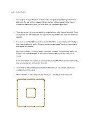
1.1. Elimination 5<br />
Figure 1.1: Forward elimination on a large matrix. The shaded boxes are<br />
nonzero entries, while zero entries are left blank. The pivots are outlined. You<br />
can see the first few steps, and then a step somewhere in the middle of the<br />
calculation, and then the final result.<br />
We are done with that pivot. Move ↘.<br />
⎛<br />
⎞<br />
3 7 4 9<br />
⎜<br />
⎟<br />
⎝ 0 1 −1 6⎠ .<br />
0 0 2 6<br />
Forward elimination is done. Lets turn the numbers back into equations, to see<br />
what we have:<br />
3x 1 +7x 2 +4x 3 = 9<br />
x 2 −x 3 = 6<br />
2x 3 = 6<br />
Each pivot solves for one variable in terms of later variables.<br />
Problem 1.1. Apply forward elimination to<br />
⎛<br />
⎞<br />
0 0 1 1<br />
0 0 1 1<br />
⎜<br />
⎟<br />
⎝1 0 3 0⎠<br />
1 1 1 1<br />
Problem 1.2. Apply forward elimination to<br />
⎛<br />
⎞<br />
1 1 0 1<br />
0 1 1 0<br />
⎜<br />
⎟<br />
⎝0 0 0 0 ⎠<br />
0 0 0 −1<br />
Back Substitution<br />
Starting at the last pivot, and working up:<br />
a. Rescale the entire row to turn the pivot into a 1.
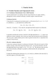
6 Solving <strong>Linear</strong> Equations<br />
Figure 1.2: Back substitution on the large matrix from figure 1.1. You can see<br />
the first few steps, and then a step somewhere in the middle of the calculation,<br />
and then the final result. You can see the pivots turn into 1’s.<br />
b. Add whatever multiples of the pivot row you need to each higher row, in<br />
order to kill off every entry above the pivot.<br />
Applied to our example:<br />
⎛<br />
⎞<br />
Scale row 3 by 1 2 :<br />
⎜<br />
⎝<br />
3 7 4 9<br />
⎟<br />
0 1 −1 6⎠ ,<br />
0 0 2 6<br />
⎛<br />
⎞<br />
3 7 4 9<br />
⎜<br />
⎟<br />
⎝ 0 1 −1 6⎠<br />
0 0 1 3<br />
Add row 3 to row 2, −4 (row 3) to row 1.<br />
⎛<br />
⎞<br />
3 7 0 −3<br />
⎜<br />
⎟<br />
⎝ 0 1 0 9 ⎠<br />
0 0 1 3<br />
Add −7 (row 2) to row 1.<br />
⎛<br />
Scale row 1 by 1 3 .<br />
⎜<br />
⎝<br />
Done. Turn back into equations:<br />
⎞<br />
3 0 0 −66<br />
⎟<br />
⎠<br />
0 1 0 9<br />
0 0 1 3<br />
⎛<br />
⎞<br />
1 0 0 −22<br />
⎜<br />
⎟<br />
⎝ 0 1 0 9 ⎠<br />
0 0 1 3<br />
x 1 = −22<br />
x 2 = 9<br />
x 3 = 3.
1.2. Examples 7<br />
Definition 1.1. Forward elimination and back substitution together are called<br />
Gauss–Jordan elimination or just elimination. (Forward elimination is often<br />
called Gaussian elimination.)<br />
Remark 1.2. Forward elimination already shows us what is going to happen:<br />
which variables are solved for in terms of which other variables. So for answering<br />
most questions, we usually only need to carry out forward elimination, without<br />
back substitution.<br />
1.2 Examples<br />
Example 1.3 (More than one solution).<br />
Write down the numbers:<br />
⎛<br />
x 1 + x 2 + x 3 + x 4 = 7<br />
x 1 + 2x 3 = 1<br />
x 2 + x 3 = 0<br />
⎞<br />
1 1 1 1 7<br />
⎜<br />
⎝ 1 0 2 0<br />
⎟<br />
1⎠ .<br />
0 1 1 0 0<br />
Kill everything under the pivot: add − (row 1) to row 2.<br />
⎛<br />
⎞<br />
1 1 1 1 7<br />
⎜<br />
⎟<br />
⎝ 0 −1 1 −1 −6⎠ .<br />
0 1 1 0 0<br />
Done with that pivot; move ↘.<br />
⎛<br />
⎞<br />
1 1 1 1 7<br />
⎜<br />
⎟<br />
⎝ 0 −1 1 −1 −6⎠ .<br />
0 1 1 0 0<br />
Kill: add row 2 to row 3:<br />
⎛<br />
⎞<br />
1 1 1 1 7<br />
⎜<br />
⎟<br />
⎝ 0 −1 1 −1 −6⎠ .<br />
0 0 2 −1 −6<br />
Move ↘. Forward elimination is done. Lets look at where the pivots lie:<br />
⎛<br />
⎞<br />
1 1 1 1 7<br />
⎜<br />
⎟<br />
⎝ 0 −1 1 −1 −6⎠ .<br />
0 0 2 −1 −6
8 Solving <strong>Linear</strong> Equations<br />
Lets turn back into equations:<br />
x 1 +x 2 +x 3 +x 4 = 7<br />
−x 2 +x 3 −x 4 =−6<br />
2x 3 −x 4 =−6<br />
Look: each pivot solves for one variable, in terms of later variables. There was<br />
never any pivot in the x 4 column, so x 4 is a free variable: x 4 can take on any<br />
value, and then we just use each pivot to solve for the other variables, bottom<br />
up.<br />
Problem 1.3. Back substitute to find the values of x 1 , x 2 , x 3 in terms of x 4 .<br />
Example 1.4 (No solutions). Consider the equations<br />
x 1 + x 2 + x 3 = 1<br />
2x 1 + x 2 + x 3 = 0<br />
4x 1 + 3x 2 + 3x 3 = 1.<br />
Forward eliminate:<br />
⎛<br />
⎞<br />
1 1 2 1<br />
⎜<br />
⎟<br />
⎝ 2 1 1 0⎠<br />
4 3 5 1<br />
Add −2(row 1) to row 2, −4(row 1) to row 3.<br />
⎛<br />
⎞<br />
1 1 2 1<br />
⎜<br />
⎟<br />
⎝ 0 −1 −3 −2⎠<br />
0 −1 −3 −3<br />
Move the pivot ↘ .<br />
⎛<br />
⎞<br />
1 1 2 1<br />
⎜<br />
⎟<br />
⎝ 0 −1 −3 −2⎠<br />
0 −1 −3 −3<br />
Add −(row 2) to row 3.<br />
⎛<br />
⎞<br />
1 1 2 1<br />
⎜<br />
⎟<br />
⎝ 0 −1 −3 −2⎠<br />
0 0 0 −1
1.3. Summary 9<br />
Move the pivot ↘ .<br />
Move the pivot →.<br />
⎛<br />
⎞<br />
1 1 2 1<br />
⎜<br />
⎟<br />
⎝ 0 −1 −3 −2⎠<br />
0 0 0 −1<br />
⎛<br />
⎜<br />
⎝<br />
1 1 2 1<br />
0 −1 −3 −2<br />
0 0 0 −1<br />
⎞<br />
⎟<br />
⎠<br />
Turn back into equations:<br />
x 1 + x 2 + 2 x 3 = 1<br />
−x 2 − 3 x 3 = −2<br />
0 = −1.<br />
You can’t solve these equations: 0 can’t equal −1. So you can’t solve the<br />
original equations either: there are no solutions. Two lessons that save you time<br />
and effort:<br />
a. If a pivot appears in the constants’ column, then there are no solutions.<br />
b. You don’t need to back substitute for this problem; forward elimination<br />
already tells you if there are any solutions.<br />
1.3 Summary<br />
We can turn linear equations into a box of numbers. Start a pivot at the top left<br />
corner, swap rows if needed, move → if swapping won’t work, kill off everything<br />
under the pivot, and then make a new pivot ↘ from the last one. After forward<br />
elimination, we will say that the resulting equations are in echelon form (often<br />
called row echelon form).<br />
The echelon form equations have the same solutions as the original equations.<br />
Each column except the last (the column of constants) represents a variable.<br />
Each pivot solves for one variable in terms of later variables (each pivot “binds”<br />
a variable, so that the variable is not free). The original equations have no<br />
solutions just when the echelon equations have a pivot in the column of constants.<br />
Otherwise there are solutions, and any pivotless column (besides the column<br />
of constants) gives a free variable (a variable whose value is not fixed by the<br />
equations). The value of any free variable can be picked as we like. So if<br />
there are solutions, there is either only one solution (no free variables), or<br />
there are infinitely many solutions (free variables). Setting free variables to<br />
different values gives different solutions. The number of pivots is called the<br />
rank. Forward elimination makes the pattern of pivots clear; often we don’t<br />
need to back substitute.
10 Solving <strong>Linear</strong> Equations<br />
Remark 1.5. We often encounter systems of linear equations for which all of<br />
the constants are zero (the “right hand sides”). When this happens, to save<br />
time we won’t write out a column of constants, since the constants would just<br />
remain zero all the way through forward elimination and back substitution.<br />
Problem 1.4. Use elimination to solve the linear equations<br />
2 x 2 + x 3 = 1<br />
4 x 1 − x 2 + x 3 = 2<br />
4 x 1 + 3 x 2 + 3 x 3 = 4<br />
1.3 Review Problems<br />
Problem 1.5. Apply forward elimination to<br />
⎛<br />
⎞<br />
2 0 2<br />
⎜<br />
⎟<br />
⎝1 0 0⎠<br />
0 2 2<br />
Problem 1.6. Apply forward elimination to<br />
⎛<br />
⎞<br />
⎜<br />
−1 −1 1 ⎟<br />
⎝ 1 1 1⎠<br />
−1 1 0<br />
Problem 1.7. Apply forward elimination to<br />
⎛<br />
⎞<br />
−1 2 −2 −1<br />
⎜<br />
⎟<br />
⎝ 1 2 −2 2 ⎠<br />
−2 0 0 −1<br />
Problem 1.8. Apply forward elimination to<br />
⎛<br />
⎞<br />
0 0 1<br />
⎜<br />
⎟<br />
⎝0 1 1⎠<br />
1 1 1<br />
Problem 1.9. Apply forward elimination to<br />
⎛<br />
⎞<br />
0 1 1 0 0<br />
0 1 0 1 0<br />
⎜<br />
⎟<br />
⎝0 0 0 0 0⎠<br />
1 1 0 1 1
1.3. Summary 11<br />
Problem 1.10. Apply forward elimination to<br />
⎛<br />
⎜<br />
1 3 2 6<br />
⎞<br />
⎟<br />
⎝2 5 4 1⎠<br />
3 8 6 7<br />
Problem 1.11. Apply back substitution to the result of problem 1.2 on page 5.<br />
Problem 1.12. Apply back substitution to<br />
⎛<br />
⎞<br />
−1 1 0<br />
⎜<br />
⎟<br />
⎝ 0 −2 0⎠<br />
0 0 1<br />
Problem 1.13. Apply back substitution to<br />
⎛<br />
⎞<br />
1 0 −1<br />
⎜<br />
⎟<br />
⎝0 −1 −1⎠<br />
0 0 0<br />
Problem 1.14. Apply back substitution to<br />
⎛<br />
⎞<br />
⎜<br />
2 1 −1 ⎟<br />
⎝0 3 −1⎠<br />
0 0 0<br />
Problem 1.15. Apply back substitution to<br />
⎛<br />
⎞<br />
3 0 2 2<br />
0 2 0 −1<br />
⎜<br />
⎟<br />
⎝0 0 3 2 ⎠<br />
0 0 0 2<br />
Problem 1.16. Use elimination to solve the linear equations<br />
−x 1 + 2 x 2 + x 3 + x 4 = 1<br />
−x 1 + 2 x 2 + 2 x 3 + x 4 = 0<br />
x 3 + 2 x 4 = 0<br />
x 4 = 2
12 Solving <strong>Linear</strong> Equations<br />
Problem 1.17. Use elimination to solve the linear equations<br />
x 1 + 2 x 2 + 3 x 3 + 4 x 4 = 5<br />
2 x 1 + 5 x 2 + 7 x 3 + 11 x 4 = 12<br />
x 2 + x 3 + 4 x 4 = 3<br />
Problem 1.18. Use elimination to solve the linear equations<br />
−2 x 1 + x 2 + x 3 + x 4 = 0<br />
x 1 − 2 x 2 + x 3 + x 4 = 0<br />
x 1 + x 2 − 2 x 3 + x 4 = 0<br />
x 1 + x 2 + x 3 − 2 x 4 = 0<br />
Problem 1.19. Write down the simplest example you can to show that adding<br />
one to each entry in a row can change the answers to the linear equations. So<br />
adding numbers to rows is not allowed.<br />
Problem 1.20. Write down the simplest systems of linear equations you can<br />
come up with that have<br />
a. One solution.<br />
b. No solutions.<br />
c. Infinitely many solutions.<br />
Problem 1.21. If all of the constants in some linear equations are zeros, must<br />
the equations have a solution?<br />
Problem 1.22. Draw the two lines 1 2 x 1 − x 2 = − 1 2 and 2 x 1 + x 2 = 3 in R 2 .<br />
In your drawing indicate the points which satisfy both equations.
1.3. Summary 13<br />
Problem 1.23. Which pair of equations cuts out which pair of lines? How<br />
many solutions does each pair of equations have?<br />
x 1 − x 2 = 0 (1)<br />
x 1 + x 2 = 1<br />
x 1 − x 2 = 4 (2)<br />
−2 x 1 + 2 x 2 = 1<br />
x 1 − x 2 = 1 (3)<br />
−3 x 1 + 3 x 2 = −3<br />
(a) (b) (c)<br />
Problem 1.24. Draw the two lines 2 x 1 + x 2 = 1 and x 1 − 2 x 2 = 1 in the<br />
x 1 x 2 -plane. Explain geometrically where the solution of this pair of equations<br />
lies. Carry out forward elimination on the pair, to obtain a new pair of equations.<br />
Draw the lines corresponding to each new equation. Explain why one of these<br />
lines is parallel to one of the axes.<br />
Problem 1.25. Find the quadratic function y = ax 2 + bx + c which passes<br />
through the points (x, y) = (0, 2), (1, 1), (2, 6).<br />
Problem 1.26. Give a simple example of a system of linear equations which<br />
has a solution, but for which, if you alter one of the coefficients by a tiny amount<br />
(as tiny as you like), then there is no solution.<br />
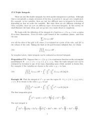
Problem 1.27. If you write down just one linear equation in three variables,<br />
like 2x 1 + x 2 − x 3 = −1, the solutions draw out a plane. So a system of three<br />
linear equations draws out three different planes. The solutions of two of the<br />
equations lie on the intersections of the two corresponding planes. The solutions<br />
of the whole system are the points where all three planes intersect. Which<br />
system of equations in table 1.1 on the next page draws out which picture of<br />
planes from figure 1.3 on page 15?
14 Solving <strong>Linear</strong> Equations<br />
x 1 − x 2 + 2 x 3 = 2 (1)<br />
−2 x 1 + 2 x 2 + x 3 = −2<br />
−3 x 1 + 3 x 2 − x 3 = 0<br />
−x 1 − x 3 = 0 (2)<br />
x 1 − 2 x 2 − x 3 = 0<br />
2 x 1 − 2 x 2 − 2 x 3 = −1<br />
x 1 + x 2 + x 3 = 1 (3)<br />
x 1 + x 2 + x 3 = 0<br />
x 1 + x 2 + x 3 = −1<br />
−2 x 1 + x 2 + x 3 = −2 (4)<br />
−2 x 1 − x 2 + 2 x 3 = 0<br />
−4 x 2 + 2 x 3 = 4<br />
−2 x 2 − x 3 = 0 (5)<br />
−x 1 − x 2 − x 3 = −1<br />
−3x 1 − 3x 2 − 3x 3 = 0<br />
Table 1.1: Five systems of linear equations
1.3. Summary 15<br />
(a) (b) (c)<br />
(d)<br />
(e)<br />
Figure 1.3: When you have three equations in three variables, each one draws a<br />
plane. Solutions of a pair of equations lie where their planes intersect. Solutions<br />
of all three equations lie where all three planes intersect.
2 Matrices<br />
The boxes of numbers we have been writing are called matrices. Lets learn the<br />
arithmetic of matrices.<br />
2.1 Definitions<br />
Definition 2.1. A matrix is a finite box A of numbers, arranged in rows and<br />
columns. We write it as<br />
⎛<br />
⎞<br />
A 11 A 12 . . . A 1q<br />
A<br />
A =<br />
21 A 22 . . . A 2q<br />
⎜<br />
⎟<br />
⎝ . . . . ⎠<br />
A p1 A p2 . . . A pq<br />
and say that A is p × q if it has p rows and q columns. If there are as many<br />
rows as columns, we will say that the matrix is square.<br />
Remark 2.2. A 31 is in row 3, column 1. If we have 10 or more rows or columns<br />
(which won’t happen in this book), we might write A 1,1 instead of A 11 . For<br />
example, we can distinguish A 11,1 from A 1,11 .<br />
Definition 2.3. A matrix x with only one column is called a vector and written<br />
⎛ ⎞<br />
x 1<br />
x<br />
x =<br />
2<br />
⎜ ⎟<br />
⎝ . ⎠ .<br />
x n<br />
The collection of all vectors with n real number entries is called R n .<br />
Think of R 2 as the xy-plane, writing each point as<br />
( )<br />
x<br />
y<br />
instead of (x, y). We draw a vector, for example the vector<br />
( )<br />
2<br />
,<br />
3<br />
17
18 Matrices<br />
⎛<br />
⎜<br />
⎝<br />
⎞<br />
⎟<br />
⎠<br />
Figure 2.1: Echelon form: a staircase, each step down by only 1, but across to<br />
the right by maybe more than one. The pivots are the steps down, and below<br />
them, in the unshaded part, are zeros.<br />
as an arrow, pointing out of the origin, with the arrow head at the point<br />
x = 2, y = 3 :<br />
Similarly, think of R 3 as 3-dimensional space.<br />
Problem 2.1. Draw the vectors:<br />
( ) ( ) ( )<br />
1 0 1<br />
, , ,<br />
0 1 1<br />
( )<br />
2<br />
,<br />
1<br />
( )<br />
3<br />
,<br />
1<br />
( )<br />
−4<br />
,<br />
2<br />
( )<br />
4<br />
.<br />
−2<br />
We draw vectors either as dots or more often as arrows. If there are too<br />
many vectors, pictures of arrows can get cluttered, so we prefer to draw dots.<br />
Sometimes we distinguish between points (drawn as dots) and vectors (drawn<br />
as arrows), but algebraically they are the same objects: columns of numbers.<br />
2.1 Review Problems<br />
Problem 2.2. Find points in R 3 which form the vertices of a regular<br />
(a) cube<br />
(b) octahedron<br />
(c) tetrahedron.<br />
2.2 Echelon Form<br />
Definition 2.4. A matrix is in echelon form if (as in figure 2.1) each row is either<br />
all zeros or starts with more zeros than any earlier row. The first nonzero entry<br />
of each row is called a pivot.
2.3. Matrices in Blocks 19<br />
Problem 2.3. Draw dots where the pivots are in figure 2.1 on the facing page.<br />
Problem 2.4. Give the simplest examples you can of two matrices which are<br />
not in echelon form, each for a different reason.<br />
Problem 2.5. The entries A 11 , A 22 , . . . of a square matrix A are called the<br />
diagonal. Prove that every square matrix in echelon form has all pivots lying<br />
on or above the diagonal.<br />
Problem 2.6. Prove that a square matrix in echelon form has a zero row just<br />
when it is either all zeroes or it has a pivot above the diagonal.<br />
Problem 2.7. Prove that a square matrix in echelon form has a column with<br />
no pivot just when it has a zero row. Thus all diagonal entries are pivots or<br />
else there is a zero row.<br />
Theorem 2.5. Forward elimination brings any matrix to echelon form, without<br />
altering the solutions of the associated linear equations.<br />
Obviously proof is by induction, but the result is clear enough, so we won’t<br />
give a proof.<br />
2.2 Review Problems<br />
Problem 2.8. In one colour, draw the locations of the pivots, and in another<br />
draw the “staircase” (as in figure 2.1 on the preceding page) for the matrices<br />
⎛<br />
(<br />
)<br />
0 1 0 1 0 ⎜<br />
1 2<br />
⎞<br />
( ) ( )<br />
⎟<br />
A =<br />
, B = ⎝0 3⎠ , C = 0 0 , D = 1 0 .<br />
0 0 0 0 1<br />
0 0<br />
2.3 Matrices in Blocks<br />
If<br />
then write<br />
(<br />
A<br />
B<br />
A =<br />
(<br />
)<br />
=<br />
(<br />
1 2<br />
3 4<br />
)<br />
and B =<br />
1 2 5 6<br />
3 4 7 8<br />
)<br />
(<br />
and<br />
5 6<br />
7 8<br />
(<br />
A<br />
B<br />
)<br />
,<br />
⎛<br />
)<br />
= ⎜<br />
⎝<br />
1 2<br />
3 4<br />
5 6<br />
7 8<br />
(We will often colour various rows and columns of matrices, just to make the<br />
discussion easier to follow. The colours have no mathematical meaning.)<br />
⎞<br />
⎟<br />
⎠ .
20 Matrices<br />
Definition 2.6. Any matrix which has only zero entries will be written 0.<br />
Problem 2.9. What could (0<br />
0) mean?<br />
Problem 2.10. What could (A 0) mean if<br />
( )<br />
1 2<br />
A = ?<br />
3 4<br />
2.4 Matrix Arithmetic<br />
Example 2.7. Add matrices like:<br />
( ) ( ) (<br />
)<br />
1 2 5 6<br />
1 + 5 2 + 6<br />
A =<br />
, B =<br />
, A + B =<br />
.<br />
3 4 7 8<br />
3 + 7 4 + 8.<br />
Definition 2.8. If two matrices have matching numbers of rows and columns,<br />
we add them by adding their components: (A + B) ij = A ij + B ij . Similarly for<br />
subtracting.<br />
Problem 2.11. Let<br />
( )<br />
1 2<br />
A =<br />
, B =<br />
3 4<br />
(<br />
−1<br />
−1<br />
)<br />
−2<br />
.<br />
−2<br />
Find A + B.<br />
When we add matrices in blocks,<br />
( ) ( )<br />
A B + C D =<br />
(<br />
A + C<br />
)<br />
B + D<br />
(as long as A and C have the same numbers of rows and columns and B and D<br />
do as well).<br />
Problem 2.12. Draw the vectors<br />
( ) ( )<br />
u =<br />
2 3<br />
, v =<br />
−1 1<br />
,<br />
and the vectors 0 and u + v. In your picture, you should see that they form the<br />
vertices of a parallelogram (a quadrilateral whose opposite sides are parallel).<br />
Multiply by numbers like:<br />
( ) (<br />
)<br />
7<br />
1 2 7 · 1 7 · 2<br />
=<br />
3 4 7 · 3 7 · 4<br />
.
2.5. Matrix Multiplication 21<br />
Definition 2.9. If A is a matrix and c is a number, cA is the matrix with<br />
(cA) ij<br />
= cA ij .<br />
Example 2.10. Let<br />
( )<br />
−1<br />
x = .<br />
2<br />
The multiples x, 2x, 3x, . . . and −x, −2x, −3x, . . . live on a straight line through<br />
0:<br />
3x<br />
2x<br />
x<br />
0<br />
−x<br />
−2x<br />
−3x<br />
2.5 Matrix Multiplication<br />
Surprisingly, matrix multiplication is more difficult.<br />
Example 2.11. To multiply a single row by a single column, just multiply entries<br />
in order, and add up:<br />
( ) ( )<br />
3<br />
1 2 = 1 · 3 + 2 · 4 = 3 + 8 = 11.<br />
4<br />
Put your left hand index finger on the row, and your right hand index finger on<br />
the column, and as you run your left hand along, run your right hand down:<br />
( ) ( )<br />
↓<br />
→ → .<br />
↓<br />
As your fingers travel, you multiply the entries you hit, and add up all of the<br />
products.<br />
Problem 2.13. Multiply<br />
⎛ ⎞<br />
(<br />
)<br />
⎜<br />
8 ⎟<br />
1 −1 2 ⎝1⎠<br />
3
22 Matrices<br />
Example 2.12. To multiply the matrices<br />
( ) ( )<br />
1 2 5 6<br />
A =<br />
, B =<br />
,<br />
3 4 7 8<br />
multiply any row of A by any column of B:<br />
(<br />
1<br />
) (<br />
2<br />
)<br />
5<br />
7<br />
=<br />
(<br />
1 · 5 + 2 · 7<br />
)<br />
.<br />
As your left hand finger travels along a row, and your right hand down a column,<br />
you produce the entry in that row and column; the second row of A times the<br />
first column of B gives the entry of AB in second row, first column.<br />
Problem 2.14. Multiply<br />
(<br />
) ⎛ ⎞<br />
1 2<br />
1 2 3 ⎜ ⎟ ⎝ 2 3⎠<br />
2 3 4<br />
3 4<br />
Definition 2.13. We write ∑ k<br />
in front of an expression to mean the sum for k<br />
taking on all possible values for which the expression makes sense. For example,<br />
if x is a vector with 3 entries,<br />
⎛ ⎞<br />
⎜<br />
x 1<br />
⎟<br />
x = ⎝x 2 ⎠ ,<br />
x 3<br />
then ∑ k x k = x 1 + x 2 + x 3 .<br />
Definition 2.14. If A is p × q and B is q × r, then AB is the p × r matrix whose<br />
entries are (AB) ij<br />
= ∑ k A ikB kj .<br />
2.5 Review Problems<br />
Problem 2.15. If A is a matrix and x a vector, what constraints on dimensions<br />
need to be satisfied to multiply Ax? What about xA?<br />
Problem 2.16.<br />
⎛ ⎞<br />
⎜<br />
2 0 ( )<br />
⎟ 0 1<br />
A = ⎝2 0⎠ , B =<br />
, C =<br />
0 1<br />
2 0<br />
Compute all of the following which are defined:<br />
AB, AC, AD, BC, CA, CD.<br />
(<br />
) ( )<br />
2 1 2<br />
0 0<br />
, D =<br />
0 1 −1 2 −1
2.5. Matrix Multiplication 23<br />
Problem 2.17. Find some 2 × 2 matrices A and B with no zero entries for<br />
which AB = 0.<br />
Problem 2.18. Find a 2 × 2 matrix A with no zero entries for which A 2 = 0.<br />
Problem 2.19. Suppose that we have a matrix A, so that whenever x is a<br />
vector with integer entries, then Ax is also a vector with integer entries. Prove<br />
that A has integer entries.<br />
Problem 2.20. A matrix is called upper triangular if all entries below the<br />
diagonal are zero. Prove that the product of upper triangular square matrices<br />
is upper triangular, and if, for example<br />
⎛<br />
⎞<br />
A 11 A 12 A 13 A 14 . . . A 1n<br />
A 22 A 23 A 24 . . . A 2n<br />
A 33 A 34 . . . A 3n<br />
A =<br />
. .. . .. ,<br />
.<br />
⎜<br />
.<br />
⎝<br />
..<br />
⎟<br />
. ⎠<br />
A nn<br />
(with zeroes under the diagonal) and<br />
⎛<br />
⎞<br />
B 11 B 12 B 13 B 14 . . . B 1n<br />
B 22 B 23 B 24 . . . B 2n<br />
B 33 B 34 . . . B 3n<br />
B =<br />
. .. . .. ,<br />
.<br />
⎜<br />
.<br />
⎝<br />
..<br />
⎟<br />
. ⎠<br />
B nn<br />
then<br />
⎛<br />
⎞<br />
A 11 B 11 ∗ ∗ ∗ . . . ∗<br />
A 22 B 22 ∗ ∗ . . . ∗<br />
A 33 B 33 ∗ . . . ∗<br />
AB =<br />
. .. . .. .<br />
.<br />
⎜<br />
.<br />
⎝<br />
..<br />
⎟<br />
∗ ⎠<br />
A nn B nn<br />
Problem 2.21. Prove the analogous result for lower triangular matrices.
24 Matrices<br />
<strong>Algebra</strong>ic Properties of Matrix Multiplication<br />
Problem 2.22. If A and B matrices, and AB is defined, and c is any number,<br />
prove that c(AB) = (cA)B = A(cB).<br />
Problem 2.23. Prove that matrix multiplication is associative: (AB)C =<br />
A(BC) (and that if either side is defined, then the other is, and they are equal).<br />
Problem 2.24. Prove that matrix multiplication is distributive: A(B + C) =<br />
AB + AC and (P + Q)R = P R + QR for any matrices A, B, C, P, Q, R (again<br />
if one side is defined, then both are and they are equal).<br />
like:<br />
etc.<br />
Running your finger along rows and columns, you see that blocks multiply<br />
( ) ( )<br />
C<br />
A B = AC + BD<br />
D<br />
Problem 2.25. To make sense of this last statement, what do we need to know<br />
about the numbers of rows and columns of A, B, C and D?
3 Important Types of Matrices<br />
Some matrices, or types of matrices, are especially important.<br />
3.1 The Identity Matrix<br />
Define matrices<br />
⎛<br />
⎞<br />
( )<br />
1 0 ⎜<br />
1 0 0 ⎟<br />
I 1 = (1) , I 2 =<br />
, I 3 = ⎝0 1 0⎠ , . . .<br />
0 1<br />
0 0 1<br />
Definition 3.1. The n × n matrix with 1’s on the diagonal and zeros everywhere<br />
else is called the identity matrix, and written I n . We often write it as I to be<br />
deliberately ambiguous about what size it is.<br />
An equivalent definition:<br />
⎧<br />
⎨<br />
1 if i = j<br />
I ij =<br />
⎩0 if i ≠ j.<br />
Problem 3.1. What could I 13 mean? (Careful: it has two meanings.) What<br />
does I 2 mean?<br />
Problem 3.2. Prove that IA = AI = A for any matrix A.<br />
Problem 3.3. Suppose that B is an n × n matrix, and that AB = A for any<br />
n × n matrix A. Prove that B = I n .<br />
Problem 3.4. If A and B are two matrices and Ax = Bx for any vector x,<br />
prove that A = B.<br />
Definition 3.2. The columns of I n are vectors called e 1 , e 2 , . . . , e n .<br />
Problem 3.5. Consider the identity matrix I 3 . What are the vectors e 1 , e 2 , e 3 ?<br />
25
26 Important Types of Matrices<br />
Problem 3.6. The vector e j has a one in which row? And zeroes in which<br />
rows?<br />
Problem 3.7. If A is a matrix, prove that Ae 1 is the first column of A.<br />
Problem 3.8. If A is any matrix, prove that Ae j is the j-th column of A.<br />
If A is a p × q matrix, by the previous exercise,<br />
A = (Ae 1 Ae 2 . . . Ae q ) .<br />
In particular, when we multiply matrices<br />
AB = (ABe 1 ABe 2 . . . ABe q )<br />
(and if either side of this equation is defined, then both sides are and they are<br />
equal). In other words, the columns of AB are A times the columns of B.<br />
This next exercise is particularly vital:<br />
Problem 3.9. If A is a matrix, and x a vector, prove that Ax is a sum of the<br />
columns of A, each weighted by entries of x:<br />
Ax = x 1 (Ae 1 ) + x 2 (Ae 2 ) + · · · + x n (Ae n ) .<br />
3.1 Review Problems<br />
Problem 3.10. True or false (if false, give a counterexample):<br />
a. If the second column of B is 3 times the first column, then the same is<br />
true of AB.<br />
b. Same question for rows instead of columns.<br />
Problem 3.11. Can you find matrices A and B so that A is 3 × 5 and B is<br />
5 × 3, and AB = I?<br />
Problem 3.12. Prove that the rows of AB are the rows of A multiplied by B.
3.1. The Identity Matrix 27<br />
(a) The<br />
original<br />
(b) (c) (d) (e)<br />
Figure 3.1: Faces formed by y = Ax. Each face is centered at the origin.<br />
Problem 3.13. The Fibonacci numbers are the numbers x 0 = 1, x 1 = 1, x n+1 =<br />
x n + x n−1 . Write down x 0 , x 1 , x 2 , x 3 and x 4 . Let<br />
( )<br />
1 1<br />
A =<br />
.<br />
1 0<br />
Prove that ( )<br />
x n+1<br />
x n<br />
( )<br />
= A n 1<br />
.<br />
1<br />
Problem 3.14. Let<br />
( ) ( )<br />
1 0<br />
x = , y = .<br />
0 2<br />
Draw these vectors in the plane. Let<br />
( ) ( ) ( )<br />
1 0 2 0 1 1<br />
A =<br />
, B =<br />
, C =<br />
,<br />
0 1 0 3 0 0<br />
( ) ( ) ( )<br />
1 0 0 0 0 −1<br />
D =<br />
, E =<br />
, F =<br />
.<br />
1 0 0 0 1 0<br />
For each matrix M = A, B, C, D, E, F draw Mx and My (in a different colour<br />
for each matrix), and explain in words what each matrix is “doing” (for example,<br />
rotating, flattening onto a line, expanding, contracting, etc.).<br />
Problem 3.15. The first picture in figure 3.1 is the original in the x 1 , x 2 plane,<br />
and the center of the circular face is at the origin. If we pick a matrix A and<br />
set y = Ax, and draw the image in the y 1 , y 2 plane, which matrix below draws<br />
which picture?
28 Important Types of Matrices<br />
( )<br />
2 0<br />
,<br />
1 0<br />
( )<br />
0 −1<br />
,<br />
1 0<br />
( )<br />
2 0<br />
,<br />
1 1<br />
( )<br />
1 0<br />
−1 1<br />
Problem 3.16. Can you figure out which matrices give rise to the pictures in<br />
the last problem, just by looking at the pictures? Assume that you known that<br />
all the entries of each matrix are integers between -2 and 2.<br />
Problem 3.17. What are the simplest examples you can find of 2 × 2 matrices<br />
A for which taking vectors x to Ax<br />
(a) contracts the plane,<br />
(b) dilates the plane,<br />
(c) dilates one direction, while contracting another,<br />
(d) rotates the plane by a right angle,<br />
(e) reflects the plane in a line,<br />
(f) moves the vertical axis, but leaves every point of the horizontal axis where<br />
it is (a “shear”)?<br />
3.2 Inverses<br />
Definition 3.3. A matrix is called square if it has the same number of rows as<br />
columns.<br />
Definition 3.4. If A is a square matrix, a square matrix B of the same size as<br />
A is called the inverse of A and written A −1 if AB = BA = I.<br />
Problem 3.18. If<br />
check that<br />
( )<br />
2 1<br />
A =<br />
,<br />
1 1<br />
( )<br />
A −1 1 −1<br />
=<br />
.<br />
−1 2<br />
Problem 3.19. If A, B and C are square matrices, and AB = I and CA = I,<br />
prove that B = C. In particular, there is only one inverse (if there is one at all).<br />
Problem 3.20. Which 1×1 matrices have inverses, and what are their inverses?<br />
Problem 3.21. By multiplying out the matrices, prove that any 2 × 2 matrix<br />
( )<br />
a b<br />
A =<br />
c d
3.2. Inverses 29<br />
has inverse<br />
as long as ad − bc ≠ 0.<br />
A −1 =<br />
(<br />
1 d<br />
ad − bc −c<br />
)<br />
−b<br />
a<br />
Problem 3.22. If A and B are invertible matrices, prove that AB is invertible,<br />
and (AB) −1 = B −1 A −1 .<br />
Problem 3.23. Prove that ( A −1) −1<br />
= A, for any invertible square matrix A.<br />
Problem 3.24. If A is invertible, prove that Ax = 0 only for x = 0.<br />
Problem 3.25. If A is invertible, and AB = I, prove that A = B −1 and<br />
B = A −1 .<br />
3.2 Review Problems<br />
Problem 3.26. Write down a pair of nonzero 2 × 2 matrices A and B for which<br />
AB = 0.<br />
Problem 3.27. If A is an invertible matrix, prove that Ax = Ay just when<br />
x = y.<br />
Problem 3.28. If a matrix M splits up into square blocks like<br />
( )<br />
A B<br />
M =<br />
0 D<br />
explain how to find M −1 in terms of A −1 and D −1 . (Warning: for a matrix<br />
which splits into blocks like<br />
( )<br />
A B<br />
M =<br />
C D<br />
the inverse of M cannot be expressed in any elementary way in terms of the<br />
blocks and their inverses.)
30 Important Types of Matrices<br />
Original<br />
Matrices<br />
Inverse matrices<br />
Figure 3.2: Images coming from some matrices, and from their inverses.<br />
Problem 3.29. Figure 3.2 shows how various matrices (on the left hand side)<br />
and their inverses (on the right hand side) affect vectors. But the two columns<br />
are scrambled up. Which right hand side picture is produced by the inverse<br />
matrix of each left hand side picture?<br />
3.3 Permutation Matrices<br />
Permutations<br />
Definition 3.5. Write down the numbers 1, 2, . . . , n in any order. Call this a<br />
permutation of the numbers 1, 2, . . . , n.
3.3. Permutation Matrices 31<br />
Problem 3.30. Suppose that I write down a list of numbers, and<br />
(a) they are all different and<br />
(b) there are 25 of them and<br />
(c) all of them are integers between 1 and 25.<br />
Prove that this list is a permutation of the numbers 1, 2, . . . , 25.<br />
We can draw a picture of a permutation: the permutation 2,4,1,3 is<br />
1 2<br />
2 4<br />
3 1<br />
4 3<br />
In general, write the numbers 1, 2, . . . , n down the left side, and the permutation<br />
down the right side, and then connect left to right, 1 to 1, 2 to 2, etc. We don’t<br />
need to write out the labels, so from now on lets draw 2,4,1,3 as<br />
Problem 3.31. Which permutations are , , ?<br />
Inverting a Permutation<br />
Definition 3.6. Flip a picture of a permutation left to right to give the inverse<br />
permutation: to . So the inverse of 2, 4, 1, 3 is 3, 1, 4, 2.<br />
Problem 3.32. Find the inverses of<br />
a. 1,2,4,3<br />
b. 4,3,2,1<br />
c. 3,1,2<br />
Multiplying<br />
We need to write down names for permutations. Write down the numbers in a<br />
permutation as p(1), p(2), . . . , p(n), and call the permutation p. If p and q are<br />
permutations, write pq for the permutation p(q(1)), p(q(2)), . . . , p(q(n)) (the<br />
product of p and q). So pq scrambles up numbers by first getting q to scramble<br />
them, and then getting p to scramble them. Multiply by drawing the pictures<br />
beside each other:<br />
p = , q = , pq = .<br />
Write the inverse permutation of p as p −1 . So pp −1 = p −1 p = 1, where 1 (the<br />
identity permutation) means the permutation that just leaves all of the numbers<br />
where they were: 1, 2, . . . , n.<br />
Problem 3.33. Let p be 2, 3, 1, 4 and q be 1, 4, 2, 3. What is pq?<br />
Problem 3.34. Write down two permutations p and q for which pq ≠ qp.
32 Important Types of Matrices<br />
Transpositions<br />
Definition 3.7. A transposition is a permutation which swaps precisely two<br />
numbers, leaving all of the others alone.<br />
For example,<br />
is a transposition.<br />
Problem 3.35. Prove that every permutation is a product of transpositions.<br />
Problem 3.36. Draw each of the following permutations as a product of<br />
transpositions:<br />
(a) 3,1,2<br />
(b) 4,3,2,1<br />
(c) 4,1,2,3<br />
Flipping the picture of a transposition left to right gives the same picture:<br />
a transposition is its own inverse. When a permutation is written as a product<br />
of transpositions, its inverse is written as the same transpositions, taken in<br />
reverse order.<br />
Problem 3.37. Prove that every permutation is a product of transpositions<br />
swapping successive numbers, i.e. swapping 1 with 2, or 2 with 3, etc.<br />
Permutation Matrices<br />
Problem 3.38. Let<br />
( )<br />
0 1<br />
P =<br />
.<br />
1 0<br />
Prove that, for any vector x in R 2 , P x is x with rows 1 and 2 swapped.<br />
Definition 3.8. The permutation matrix associated to a permutation p of the<br />
numbers 1, 2, . . . , n is<br />
)<br />
P =<br />
(e p(1) e p(2) . . . e p(n) .<br />
Example 3.9. Let p be the permutation 3, 1, 2. The permutation matrix of p is<br />
⎛<br />
⎞<br />
) 0 1 0<br />
⎜<br />
⎟<br />
P =<br />
(e 3 e 1 e 2 = ⎝0 0 1⎠ .<br />
1 0 0<br />
Problem 3.39. What is the permutation matrix P associated to the permutation<br />
4, 2, 5, 3, 1?
3.3. Permutation Matrices 33<br />
Problem 3.40. What permutation p has permutation matrix<br />
⎛<br />
⎞<br />
0 0 1 0<br />
1 0 0 0<br />
⎜<br />
⎟<br />
⎝0 1 0 0⎠ ?<br />
0 0 0 1<br />
Problem 3.41. What is the permutation matrix of the identity permutation?<br />
Problem 3.42. Prove that a matrix is the permutation matrix of some permutation<br />
just when<br />
a. its entries are all 0’s or 1’s and<br />
b. it has exactly one 1 in each column and<br />
c. it has exactly one 1 in each row.<br />
Lemma 3.10. Let P be the permutation matrix associated to a permutation p.<br />
Then for any vector x, P x is just x with the x 1 entry moved to row p(1), the<br />
x 2 entry moved to row p(2), etc.<br />
Remark 3.11. All we need to remember is that P x is x with rows permuted<br />
somehow, and that we could permute the rows of x any way we want by<br />
choosing a suitable permutation matrix P . We will never have to actually find<br />
the permutation.<br />
Proof.<br />
P x = P ∑ j<br />
x j e j<br />
= ∑ j<br />
= ∑ j<br />
x j P e j<br />
x j e p(j) .<br />
Proposition 3.12. Let P be the permutation matrix associated to a permutation<br />
p. Then for any matrix A, P A is just A with the row 1 moved to row p(1), row<br />
2 moved to row p(2), etc.<br />
Proof. The columns of P A are just P multiplied by the columns of A.<br />
Remark 3.13. It is faster and easier to work directly with permutations than<br />
with permutation matrices. Avoid writing down permutation matrices if you<br />
can; otherwise you end up wasting time juggling huge numbers of 0’s. Replace<br />
permutation matrices by permutations.
34 Important Types of Matrices<br />
Problem 3.43. If p and q are two permutations with permutation matrices P<br />
and Q, prove that pq has permutation matrix P Q.<br />
3.3 Review Problems<br />
Problem 3.44. Let<br />
⎛<br />
⎞<br />
0 1 2<br />
⎜<br />
⎟<br />
A = ⎝0 0 0⎠ .<br />
3 0 0<br />
Which permutation p do we need to make sure that P A is in echelon form, with<br />
P the permutation matrix of p?<br />
Problem 3.45. Confusing: Prove that the permutation matrix P of a permutation<br />
p is the result of permuting the columns of the identity matrix by p, or<br />
the rows of the identity matrix by p −1 .<br />
Problem 3.46. What happens to a permutation matrix when you carry out<br />
forward elimination? back substitution?<br />
Problem 3.47. Let p be a permutation with permutation matrix P . Prove<br />
that P −1 is the permutation matrix of p −1 .
4 Elimination Via Matrix<br />
Arithmetic<br />
In this chapter, we will describe linear equations and elimination using only<br />
matrix multiplication.<br />
4.1 Strictly Lower Triangular Matrices<br />
Definition 4.1. A square matrix is strictly lower triangular if it has the form<br />
⎛<br />
⎞<br />
1<br />
1<br />
S =<br />
⎜<br />
.<br />
⎝<br />
.. ⎟<br />
⎠<br />
1<br />
with 1’s on the diagonal, 0’s above the diagonal, and anything below.<br />
Problem 4.1. Let S be strictly lower triangular. Must it be true that S ij = 0<br />
for i > j? What about for j > i?<br />
Lemma 4.2. If S is a strictly lower triangular matrix, and A any matrix, then<br />
SA is A with S ij (row j) added to row i. In particular, S adds multiples of rows<br />
to lower rows.<br />
Proof. For x a vector,<br />
⎛<br />
1<br />
S<br />
Sx =<br />
21 1<br />
⎜<br />
⎝<br />
S 31 S 32 1<br />
. . .<br />
. . .<br />
⎛<br />
x 1<br />
⎞<br />
x<br />
=<br />
2 + S 21 x 1<br />
⎜<br />
⎝<br />
x 3 + S 31 x 1 + S 32 x 2<br />
⎟<br />
⎠<br />
.<br />
⎞ ⎛<br />
⎟ ⎜<br />
⎠ ⎝<br />
. ..<br />
x 1<br />
x 2<br />
x 3<br />
.<br />
⎞<br />
⎟<br />
⎠<br />
35
36 Elimination Via Matrix Arithmetic<br />
adds S 21 x 1 to x 2 , etc.<br />
If A is any matrix then the columns of SA are S times columns of A.<br />
Problem 4.2. Let S be a matrix so that for any matrix A (of appropriate<br />
size), SA is A with multiples of some rows added to later rows. Prove that S is<br />
strictly lower triangular.<br />
Problem 4.3. Which 3 × 3 matrix S adds −5 row 2 to row 3, and −7 row 1 to<br />
row 2?<br />
Problem 4.4. Prove that if R and S are strictly lower triangular, then RS is<br />
too.<br />
Problem 4.5. Say that a strictly lower triangular matrix is elementary if it<br />
has only one nonzero entry below the diagonal. Prove that every strictly lower<br />
triangular matrix is a product of elementary strictly lower triangular matrices.<br />
Lemma 4.3. Every strictly lower triangular matrix is invertible, and its inverse<br />
is also strictly lower triangular.<br />
Proof. Clearly true for 1 × 1 matrices. Lets consider an n × n strictly lower<br />
triangular matrix S, and assume that we have already proven the result for all<br />
matrices of smaller size. Write<br />
S =<br />
(<br />
1 0<br />
c A<br />
where c is a column and A is a smaller strictly lower triangular matrix. Then<br />
(<br />
)<br />
S −1 =<br />
1 0<br />
−A −1 c A −1 ,<br />
which is strictly lower triangular.<br />
Definition 4.4. A matrix M is strictly upper triangular if it has ones down the<br />
diagonal zeroes everywhere below the diagonal.<br />
Problem 4.6. For each fact proven above about strictly lower triangular<br />
matrices, prove an analogue for strictly upper triangular matrices.<br />
)
4.2. Diagonal Matrices 37<br />
Problem 4.7. Draw a picture indicating where some vectors lie in the x 1 x 2<br />
plane, and where they get mapped to in the y 1 y 2 plane by y = Ax with<br />
( )<br />
1 0<br />
A =<br />
.<br />
2 1<br />
4.2 Diagonal Matrices<br />
A diagonal matrix is one like<br />
⎛<br />
⎞<br />
t 1 t<br />
D =<br />
2 ⎜<br />
.<br />
⎝<br />
.. ⎟<br />
⎠ ,<br />
t n<br />
(with blanks representing 0 entries).<br />
Problem 4.8. Show by calculation that<br />
⎛<br />
1<br />
⎜<br />
⎝<br />
1<br />
⎞ ⎛<br />
⎞ ⎛<br />
⎞<br />
1 2 3 1 2 3<br />
⎟ ⎜<br />
⎟ ⎜<br />
⎟<br />
⎠ ⎝4 5 6⎠ = ⎝4 5 6⎠ .<br />
7 8 9<br />
1<br />
7<br />
1<br />
8<br />
7<br />
9<br />
7<br />
Problem 4.9. Prove that a diagonal matrix D is invertible just when none of<br />
its diagonal entries are zero. Find its inverse.<br />
Lemma 4.5. If<br />
⎛<br />
⎞<br />
t 1 t<br />
D =<br />
2 ⎜<br />
.<br />
⎝<br />
.. ⎟<br />
⎠ ,<br />
t n<br />
then DA is A with row 1 scaled by t 1 , etc.
38 Elimination Via Matrix Arithmetic<br />
Proof. For a vector x,<br />
⎛<br />
⎞ ⎛ ⎞<br />
t 1 x 1<br />
t<br />
Dx =<br />
2 x 2<br />
⎜<br />
.<br />
⎝<br />
.. ⎟ ⎜ ⎟<br />
⎠ ⎝ . ⎠<br />
t n x n<br />
⎛ ⎞<br />
t 1 x 1<br />
t<br />
=<br />
2 x 2<br />
⎜ ⎟<br />
⎝ . ⎠<br />
t n x n<br />
(just running your fingers along rows and down columns). So D scales row i by<br />
t i . For any matrix A, the columns of DA are D times columns of A.<br />
4.2 Review Problems<br />
Problem 4.10. Which diagonal matrix D takes the matrix<br />
( )<br />
3 4<br />
A =<br />
5 6<br />
to the matrix<br />
( )<br />
DA =<br />
4<br />
1<br />
3<br />
5 6<br />
?<br />
Problem 4.11. Multiply<br />
⎛<br />
⎞ ⎛<br />
⎞<br />
⎜<br />
a 0 0 d 0 0<br />
⎟ ⎜<br />
⎟<br />
⎝0 b 0⎠<br />
⎝0 e 0⎠<br />
0 0 c 0 0 f<br />
Problem 4.12. Draw a picture indicating where some vectors lie in the x 1 x 2<br />
plane, and where they get mapped to in the y 1 y 2 plane by y = Ax with each of<br />
the following matrices playing the part of A:<br />
( )<br />
2 0<br />
,<br />
0 3<br />
( )<br />
1 0<br />
,<br />
0 −1<br />
( )<br />
2 0<br />
.<br />
0 −3
4.3. Encoding <strong>Linear</strong> Equations in Matrices 39<br />
4.3 Encoding <strong>Linear</strong> Equations in Matrices<br />
<strong>Linear</strong> equations<br />
x 2 − x 3 = 6<br />
3x 1 + 7x 2 + 4x 3 = 9<br />
3x 1 + 5x 2 + 8x 3 = 3<br />
can be written in matrix form as<br />
⎛<br />
⎞ ⎛ ⎞ ⎛ ⎞<br />
0 1 −1<br />
⎜<br />
⎟ ⎜<br />
x 1 6<br />
⎟ ⎜ ⎟<br />
⎝3 7 4 ⎠ ⎝x 2 ⎠ = ⎝9⎠ .<br />
3 5 8 x 3 3<br />
Any linear equations<br />
A 11 x 1 + A 12 x 2 + · · · + A 1q x q = b 1<br />
A 21 x 1 + a 22 x 2 + · · · + A 2q x q = b 2<br />
. = . .<br />
A p1 x 1 + A p2 x 2 + · · · + A pq x q = b p<br />
become ⎛<br />
⎞ ⎛ ⎞ ⎛ ⎞<br />
A 11 A 12 . . . A 1q x 1 b 1<br />
A 21 A 22 . . . A 2q<br />
x 2<br />
⎜<br />
.<br />
⎝ . . .. ⎟ ⎜ ⎟ . ⎠ ⎝ . ⎠ = b 2 ⎜ ⎟<br />
⎝ . ⎠<br />
A p1 A p2 . . . A pq x q b p<br />
which we write as Ax = b.<br />
Problem 4.13. Write the linear equations<br />
x 1 + 2 x 2 = 7<br />
3 x 1 + 4 x 2 = 8<br />
in matrices.<br />
4.4 Forward Elimination Encoded in Matrix Multiplication<br />
Forward elimination on a matrix A is carried out by multiplying on the left of<br />
A by a sequence of permutation matrices and strictly lower triangular matrices.<br />
Example 4.6.<br />
⎛<br />
⎞<br />
⎜<br />
0 1 −1 ⎟<br />
A = ⎝3 7 4 ⎠<br />
3 5 8
40 Elimination Via Matrix Arithmetic<br />
Swap rows 1 and 2 (and lets write out the permutation matrix):<br />
⎛<br />
⎞ ⎛<br />
⎞<br />
0 1 0 3 7 4<br />
⎜<br />
⎟ ⎜<br />
⎟<br />
⎝1 0 0⎠ A = ⎝ 0 1 −1⎠<br />
0 0 1 3 5 8<br />
Add − (row 1) to (row 3):<br />
⎛<br />
⎞ ⎛<br />
⎞ ⎛<br />
⎞<br />
1 0 0<br />
⎜<br />
⎟ ⎜<br />
0 1 0 3 7 4<br />
⎟ ⎜<br />
⎟<br />
⎝ 0 1 0⎠<br />
⎝1 0 0⎠ A = ⎝ 0 1 −1⎠<br />
−1 0 1 0 0 1 0 −2 4<br />
The string of matrices in front of A just gets longer at each step. Add 2 (row 2)<br />
to (row 3).<br />
⎛<br />
⎞ ⎛<br />
⎞ ⎛<br />
⎞ ⎛<br />
⎞<br />
⎜<br />
1 0 0 1 0 0 0 1 0 3 7 4<br />
⎟ ⎜<br />
⎟ ⎜<br />
⎟ ⎜<br />
⎟<br />
⎝0 1 0⎠<br />
⎝ 0 1 0⎠<br />
⎝1 0 0⎠ A = ⎝ 0 1 −1⎠<br />
0 2 1 −1 0 1 0 0 1 0 0 2<br />
Call this U. This is the echelon form:<br />
⎛<br />
⎞ ⎛<br />
⎞ ⎛<br />
⎞<br />
1 0 0 1 0 0<br />
⎜<br />
⎟ ⎜<br />
⎟ ⎜<br />
0 1 0 ⎟<br />
U = ⎝0 1 0⎠<br />
⎝ 0 1 0⎠<br />
⎝1 0 0⎠ A.<br />
0 2 1 −1 0 1 0 0 1<br />
Remark 4.7. We won’t write out these tedious matrices on the left side of A<br />
ever again, but it is important to see it done once.<br />
Remark 4.8. Back substitution is similarly carried out by multiplying by strictly<br />
upper triangular and invertible diagonal matrices.<br />
4.4 Review Problems<br />
Problem 4.14. Let P be the 3 × 3 permutation matrix which swaps rows 1<br />
and 2. What does the matrix P 99 do? Write it down.<br />
Problem 4.15. Let S be the 3 × 3 strictly lower triangular matrix which adds<br />
2 (row 1) to row 3. What does the 3 × 3 matrix S 101 do? Write it down.<br />
Problem 4.16. Which 3 × 3 matrix adds twice the first row to the second row<br />
when you multiply by it?<br />
Problem 4.17. Which 4 × 4 matrix swaps the second and fourth rows when<br />
you multiply by it?
4.4. Forward Elimination Encoded in Matrix Multiplication 41<br />
Problem 4.18. Which 4 × 4 matrix doubles the second and quadruples the<br />
third rows when you multiply by it?<br />
Problem 4.19. If P is the permutation matrix of a permutation p, what is<br />
AP ?<br />
Problem 4.20. If we start with<br />
⎛<br />
⎞<br />
⎜<br />
0 0 1 ⎟<br />
A = ⎝2 3 4⎠<br />
0 5 6<br />
and end up with<br />
what permutation matrix is P ?<br />
⎛<br />
⎞<br />
⎜<br />
2 3 4 ⎟<br />
P A = ⎝0 5 6⎠<br />
0 0 1<br />
Problem 4.21. If A is a 2×2 matrix, and AP = P A for every 2×2 permutation<br />
matrix P or strictly lower triangular matrix, then prove that A = c I for some<br />
number c.<br />
Problem 4.22. If the third and fourth columns of a matrix A are equal, are<br />
they still equal after we carry out forward elimination? After back substitution?<br />
Problem 4.23. How many pivots can there be in a 3 × 5 matrix in echelon<br />
form?<br />
Problem 4.24. Write down the simplest 3 × 5 matrices you can come up with<br />
in echelon form and for which<br />
a. The second and third variables are the only free variables.<br />
b. There are no free variables.<br />
c. There are pivots in precisely the columns 3 and 4.<br />
Problem 4.25. Write down the simplest matrices A you can for which the<br />
number of solutions to Ax = b is<br />
a. 1 for any b;<br />
b. 0 for some b, and ∞ for other b;<br />
c. 0 for some b, and 1 for other b;<br />
d. ∞ for any b.<br />
Problem 4.26. Suppose that A is a square matrix. Prove that all entries of A<br />
are positive just when, for any nonzero vector x which has no negative entries,<br />
the vector Ax has only positive entries.
42 Elimination Via Matrix Arithmetic<br />
Problem 4.27. Prove that short matrices kill. A matrix is called short if it<br />
is wider than it is tall. We say that a matrix A kills a vector x if x ≠ 0 but<br />
Ax = 0.<br />
4.5 Summary<br />
The many steps of elimination can each be encoded into a matrix multiplication.<br />
The resulting matrices can all be multiplied together to give the single equation<br />
U = V A, where A is the matrix we started with, U is the echelon matrix we<br />
end up with and V is the product of the various matrices that carry out all<br />
of our elimination steps. There is a big idea at work here: encode a possibly<br />
huge number of steps into a single algebraic equation (in this case the equation<br />
U = V A), turning a large computation into a simple piece of algebra. We will<br />
return to this idea periodically.
5 Finding the Inverse of a Matrix<br />
Lets use elimination to calculate the inverse of a matrix.<br />
5.1 Finding the Inverse of a Matrix By Elimination<br />
Example 5.1. If Ax = y then multiplying both sides by A −1 gives x = A −1 y,<br />
solving for x. We can write out Ax = y as linear equations, and solve these<br />
equations for x. For example, if<br />
( )<br />
1 −2<br />
A =<br />
,<br />
2 −3<br />
then writing out Ax = y:<br />
x 1 −2 x 2 = y 1<br />
2 x 1 −3 x 2 = y 2 .<br />
Let apply Gauss–Jordan elimination, but watch the equations instead of the<br />
matrices. Add -2(equation 1) to equation 2.<br />
Add 2(equation 2) to equation 1.<br />
x 1 −2 x 2 = y 1<br />
x 2 = −2 y 1 + y 2 .<br />
x 1 = −3 y 1 + 2 y 2<br />
x 2 = −2 y 1 + y 2 .<br />
So<br />
( )<br />
A −1 −3 2<br />
=<br />
.<br />
−2 1<br />
Theorem 5.2. Let A be a square matrix. Suppose that Gauss–Jordan elimination<br />
applied to the matrix (A I) ends up with (U V ) with U and V square<br />
matrices. A is invertible just when U = I, in which case V = A −1 .<br />
43
44 Finding the Inverse of a Matrix<br />
Example 5.3. Before the proof, lets have an example. Lets invert<br />
( )<br />
1 −2<br />
A =<br />
.<br />
2 −3<br />
(<br />
A<br />
I<br />
(<br />
)<br />
=<br />
1 −2 1 0<br />
2 −3 0 1<br />
)<br />
Add -2(row 1) to row 2.<br />
(<br />
1 −2 1 0<br />
0 1 −2 1<br />
)<br />
Make a new pivot ↘.<br />
(<br />
1 −2 1 0<br />
0 1 −2 1<br />
)<br />
Add 2(row 2) to row 1.<br />
(<br />
1 0 −3 2<br />
0<br />
(<br />
1 −2<br />
)<br />
1<br />
= U V .<br />
)<br />
Obviously these are the same steps we used in the example above; the shaded<br />
part represents coefficients in front of the y vector above. Since U = I, A is<br />
invertible and<br />
A −1 = V<br />
( )<br />
−3 2<br />
=<br />
.<br />
−2 1<br />
Proof. Gauss–Jordan elimination on (A I) is carried out by multiplying by<br />
various invertible matrices (strictly lower triangular, permutation, invertible<br />
diagonal and strictly upper triangular), say like<br />
( ) ( )<br />
U V = M N M N−1 . . . M 2 M 1 A I .<br />
So<br />
U = M N M N−1 . . . M 2 M 1 A<br />
V = M N M N−1 . . . M 2 M 1 ,
5.1. Finding the Inverse of a Matrix By Elimination 45<br />
which we summarize as U = V A. Clearly V is a product of invertible matrices,<br />
so invertible. Thus U is invertible just when A is.<br />
First suppose that U has pivots all down the diagonal. Every pivot is a 1.<br />
Entries above and below each pivot are 0, so U = I. Since U = V A, we find<br />
I = V A. Multiply both sides on the left by V −1 , to see that V −1 = A. But<br />
then multiply on the right by V to see that I = AV . So A and V are inverses<br />
of one another.<br />
Next suppose that U doesn’t have pivots all down the diagonal. We always<br />
start Gauss–Jordan elimination on the diagonal, so we fail to place a pivot somewhere<br />
along the diagonal just because we move → during forward elimination.<br />
That move makes a pivotless column, hence a free variable for the equation<br />
Ax = 0. Setting the free variable to a nonzero value produces a nonzero x with<br />
Ax = 0. By problem 3.24 on page 29, A is not invertible.<br />
Problem 5.1. Find the inverse of<br />
⎛<br />
⎜<br />
0 0 1<br />
⎞<br />
⎟<br />
A = ⎝1 1 0⎠ .<br />
1 2 1<br />
5.1 Review Problems<br />
Problem 5.2. Find the inverse of<br />
⎛<br />
⎞<br />
⎜<br />
1 2 3 ⎟<br />
A = ⎝1 2 0⎠ .<br />
1 0 0<br />
Problem 5.3. Find the inverse of<br />
⎛<br />
⎞<br />
1 −1 1<br />
⎜<br />
⎟<br />
A = ⎝−1 1 −1⎠ .<br />
1 −1 1<br />
Problem 5.4. Find the inverse of<br />
⎛<br />
⎜<br />
1 1 1<br />
⎞<br />
⎟<br />
A = ⎝0 1 3⎠ .<br />
1 1 3<br />
Problem 5.5. Is there a faster method than Gauss–Jordan elimination to find<br />
the inverse of a permutation matrix?
46 Finding the Inverse of a Matrix<br />
5.2 Invertibility and Forward Elimination<br />
Proposition 5.4. A square matrix U in echelon form is invertible just when<br />
U has pivots all the way down the diagonal, which occurs just when U has no<br />
zero rows.<br />
Proof. Applying back substitution to a matrix U which is already in echelon<br />
form preserves the locations of the pivots, and just rescales them to be 1, killing<br />
everything above them. So back substitution takes U to I just when U has<br />
pivots all the way down the diagonal.<br />
Example 5.5. (<br />
is invertible, while<br />
is not invertible.<br />
)<br />
1 2<br />
0 7<br />
⎛<br />
⎞<br />
⎜<br />
0 1 2 ⎟<br />
⎝0 0 3 ⎠<br />
0 0 0<br />
Theorem 5.6. A square matrix A is invertible just when its echelon form U<br />
is invertible.<br />
Remark 5.7. So we can quickly decide if a matrix is invertible by forward<br />
elimination. We only need back substitution if we actually need to compute<br />
out the inverse.<br />
Proof. U = V A, and V is invertible, so U is invertible just when A is.<br />
Example 5.8.<br />
has echelon form<br />
so A is invertible.<br />
( )<br />
0 1<br />
A =<br />
1 1<br />
U =<br />
(<br />
)<br />
1 1<br />
0 1<br />
Problem 5.6. Is ( )<br />
0 1<br />
1 0<br />
invertible?
5.2. Invertibility and Forward Elimination 47<br />
Problem 5.7. Is<br />
invertible?<br />
⎛<br />
⎞<br />
⎜<br />
0 1 0 ⎟<br />
⎝1 0 1⎠<br />
1 1 1<br />
Problem 5.8. Prove that a square matrix A is invertible just when the only<br />
solution x to the equation Ax = 0 is x = 0.<br />
Inversion and Solvability of <strong>Linear</strong> Equations<br />
Theorem 5.9. Take a square matrix A. The equation Ax = b has a solution x<br />
for every vector b just when A is invertible. For each b, the solution x is then<br />
unique. On the other hand, if A is not invertible, then Ax = b has either no<br />
solution or infinitely many, and both of these possibilities occur for different<br />
choices of b.<br />
Proof. If A is invertible, then multiplying both sides of Ax = b by A −1 , we see<br />
that we have to have x = A −1 b.<br />
On the other hand, suppose that A is not invertible. There is a free variable<br />
for Ax = b, so no solutions or infinitely many. Lets see that for different choices<br />
of b both possibilities occur. Carry out forward elimination, say U = V A. Then<br />
U has a zero row, say row n. We can’t solve Ux = e n (look at row n). So<br />
set b = V −1 e n and we can’t solve Ax = b. But now instead set b = 0 and we<br />
can solve Ax = 0 (for example with x = 0) and therefore solve Ax = 0 with<br />
infinitely many solutions x, since there is a free variable.<br />
Example 5.10. The equations<br />
x 1 + 2x 2 = 9845039843453455938453<br />
x 1 − 2x 2 = 90853809458394034464578<br />
have a unique solution, because they are Ax = b with<br />
( )<br />
1 2<br />
A =<br />
1 −2<br />
which has echelon form<br />
U =<br />
(<br />
)<br />
1 2<br />
.<br />
0 −4
48 Finding the Inverse of a Matrix<br />
Problem 5.9. Suppose that A and B are n × n matrices and AB = I. Prove<br />
that A and B are both invertible, and that B = A −1 and that A = B −1 .<br />
Problem 5.10. Prove that for square matrices A and B of the same size<br />
(AB) −1 = B −1 A −1<br />
(and if either side is defined, then the other is and they are equal).<br />
5.2 Review Problems<br />
Problem 5.11. Is<br />
invertible?<br />
( )<br />
0 −1<br />
A =<br />
1 0<br />
Problem 5.12. How many solutions are there to the following equations?<br />
x 1 + 2x 2 + 3x 3 = 284905309485083<br />
x 1 + 2x 2 + x 3 = 92850234853408<br />
x 2 + 15x 3 = 4250348503489085.<br />
Problem 5.13. Let A be the n × n matrix which has 1 in every entry on or<br />
under the diagonal, and 0 in every entry above the diagonal. Find A −1 .<br />
Problem 5.14. Let A be the n × n matrix which has 1 in every entry on or<br />
above the diagonal, and 0 in every entry below the diagonal. Find A −1 .<br />
Problem 5.15. Give an example of a 3 × 3 invertible matrix A for which A<br />
and A t have different values for their pivots.<br />
Problem 5.16. Imagine that you start with a matrix A which might not be<br />
invertible, and carry out forward elimination on (A I). Suppose you arrive at<br />
⎛<br />
⎞<br />
∗ ∗ ∗ ∗ ∗ ∗ ∗ ∗<br />
∗ ∗ ∗ ∗ ∗ ∗ ∗ ∗<br />
(U V ) = ⎜<br />
⎟<br />
⎝0 0 0 0 2 8 3 9⎠ ,<br />
0 0 0 0 0 1 5 2
5.2. Invertibility and Forward Elimination 49<br />
with some pivots somewhere on the first two rows of U. Fact: you can solve<br />
Ax = b just for those vectors b which solve the equations<br />
Explain why.<br />
2b 1 +8b 2 +3b 3 +9b 4 = 0<br />
b 2 +5b 3 +2b 4 = 0 .
6 The Determinant<br />
We can see whether a matrix is invertible by computing a single number, the<br />
determinant.<br />
Problem 6.1. Use forward elimination to prove that a 2 × 2 matrix<br />
( )<br />
a b<br />
A =<br />
c d<br />
is invertible just when ad − bc ≠ 0.<br />
( )<br />
a b<br />
For any 2 × 2 matrix<br />
, the determinant is ad − bc. For larger<br />
c d<br />
matrices, the determinant is complicated.<br />
6.1 Definition<br />
Determinants are computed as in figure 6.1 on the next page. To compute<br />
a determinant, run your finger down the first column, writing down plus and<br />
minus signs in the pattern +, −, +, −, . . . in front the entry your finger points<br />
at, and then writing down the determinant of the matrix you get by deleting<br />
the row and column where your finger lies (always the first column), and add<br />
up.<br />
Problem 6.2. Prove that<br />
det<br />
(<br />
a<br />
c<br />
)<br />
b<br />
= ad − bc.<br />
d<br />
6.1 Review Problems<br />
Problem 6.3. Find the determinant of<br />
( )<br />
3 1<br />
1 −3<br />
51
52 The Determinant<br />
⎛<br />
⎞<br />
⎛<br />
⎜<br />
3 2 1 ⎟<br />
⎜<br />
det ⎝1 4 5⎠ = + (3) det ⎝<br />
6 7 2<br />
⎛<br />
⎜<br />
− (1) det ⎝<br />
⎛<br />
⎜<br />
+ (6) det ⎝<br />
=3 det<br />
(<br />
4 5<br />
7 2<br />
3 2 1<br />
1 4 5<br />
6 7 2<br />
3 2 1<br />
1 4 5<br />
6 7 2<br />
3 2 1<br />
1 4 5<br />
6 7 2<br />
)<br />
− det<br />
(<br />
⎞<br />
⎟<br />
⎠<br />
⎞<br />
⎟<br />
⎠<br />
⎞<br />
⎟<br />
⎠<br />
2 1<br />
7 2<br />
) ( )<br />
2 1<br />
+ 6 det<br />
4 5<br />
Figure 6.1: Computing a 3 × 3 determinant.<br />
Problem 6.4. Find the determinant of<br />
⎛<br />
⎞<br />
⎜<br />
1 −1 0 ⎟<br />
⎝0 1 1 ⎠<br />
1 0 −1<br />
Problem 6.5. Does A 2 11 appear in the expression for det A, when you expand<br />
out all of the determinants in the expression completely?<br />
Problem 6.6. Prove that the determinant of<br />
⎛<br />
∗ ∗ ∗ ∗ ∗ ∗ ∗ ∗<br />
0 0 0 ∗ ∗ ∗ ∗ ∗<br />
0 0 0 ∗ ∗ ∗ ∗ ∗<br />
A =<br />
0 0 0 ∗ ∗ ∗ ∗ ∗<br />
0 0 0 ∗ ∗ ∗ ∗ ∗<br />
0 0 0 ∗ ∗ ∗ ∗ ∗<br />
⎜<br />
⎝ 0 0 0 ∗ ∗ ∗ ∗ ∗<br />
∗ ∗ ∗ ∗ ∗ ∗ ∗ ∗<br />
⎞<br />
⎟<br />
⎠<br />
is zero, no matter what number we put in place of the ∗’s, even if the numbers<br />
are all different.
6.2. Easy Determinants 53<br />
Problem 6.7. Give an example of a matrix all of whose entries are positive,<br />
even though its determinant is zero.<br />
Problem 6.8. What is det I? Justify your answer.<br />
Problem 6.9. Prove that<br />
( )<br />
A B<br />
det<br />
= det A det C,<br />
0 C<br />
for A and C any square matrices, and B any matrix of appropriate size to fit<br />
in here.<br />
6.2 Easy Determinants<br />
Example 6.1. Lets find the determinant of<br />
⎛<br />
7<br />
⎜<br />
A = ⎝ 4<br />
⎞<br />
⎟<br />
⎠ .<br />
2<br />
(There are zeros wherever entries are not written.) Running down the first<br />
column, we only hit the 7. So<br />
( )<br />
4<br />
det A = 7 det .<br />
2<br />
By the same trick:<br />
Summing up:<br />
det A = (7)(4) det(2)<br />
= (7)(4)(2).<br />
Lemma 6.2. The determinant of a diagonal matrix<br />
⎛<br />
⎞<br />
p 1 p<br />
A =<br />
2 ⎜<br />
.<br />
⎝<br />
.. ⎟<br />
⎠<br />
p n<br />
is det A = p 1 p 2 . . . p n .<br />
We can easily do better: recall that a matrix A is upper triangular if all<br />
entries below the diagonal are 0. By the same trick again:
54 The Determinant<br />
Lemma 6.3. The determinant of an upper triangular square matrix<br />
⎛<br />
⎞<br />
U 11 U 12 U 13 U 14 . . . U 1n<br />
U 22 U 23 U 24 . . . U 2n<br />
U 33 U 34 . . . U 3n<br />
U =<br />
. .. . .. .<br />
⎜<br />
.<br />
⎝<br />
..<br />
⎟<br />
. ⎠<br />
U nn<br />
is the product of the diagonal terms: det U = U 11 U 22 . . . U nn .<br />
Corollary 6.4. A square matrix A is invertible just when det U ≠ 0, with U<br />
obtained from A by forward elimination.<br />
Proof. The matrix U is upper triangular. The fact that det U ≠ 0 says just<br />
precisely that all diagonal entries of U are not zero, so are pivots—a pivot in<br />
every column. Apply theorem 5.6 on page 46.<br />
6.2 Review Problems<br />
Problem 6.10. Find<br />
⎛<br />
⎞<br />
1 2 3<br />
⎜<br />
⎟<br />
det ⎝0 4 5⎠ .<br />
0 0 6<br />
Problem 6.11. Suppose that U is an invertible upper triangular matrix.<br />
a. Prove that U −1 is upper triangular.<br />
b. Prove that the diagonal entries of U −1 are the reciprocals of the diagonal<br />
entries of U.<br />
c. How can you calculate by induction the entries of U −1 in terms of the<br />
entries of U?<br />
Problem 6.12. Let U be any upper triangular matrix with integer entries.<br />
Prove that U −1 has integer entries just when det U = ±1.<br />
6.3 Tricks to Find Determinants<br />
Lemma 6.5. Swapping any two neighbouring rows of a square matrix changes<br />
the sign of the determinant. For example,<br />
( ) ( )<br />
1 2<br />
3 4<br />
det<br />
= − det<br />
.<br />
3 4<br />
1 2
6.3. Tricks to Find Determinants 55<br />
Proof. It is obvious for 1 × 1 (you can’t swap anything). It is easy to check for<br />
a 2 × 2. Picture a 3 × 3 matrix A (like example 6.1 on page 52). For simplicity,<br />
lets swap rows 1 and 2. Then the plus sign of row 1 and the minus sign of row<br />
2 are clearly switched in the 1st and 2nd terms in the determinant. In the 3rd<br />
term, the leading plus sign is not switched. Look at the determinant in the<br />
3rd term: rows 1 and 2 don’t get crossed out, and have been switched, so the<br />
determinant factor changes sign. So all terms in the determinant formula have<br />
changed sign, and therefore the determinant has changed sign. The argument<br />
goes through identically with any size of matrix (by induction) and any two<br />
neighboring rows, instead of just rows 1 and 2.<br />
Lemma 6.6. Swapping any two rows of a square matrix changes the sign<br />
of the determinant, so det P A = − det A for P the permutation matrix of a<br />
transposition.<br />
Proof. Suppose that we want to swap two rows, not neighboring. For concreteness,<br />
imagine rows 1 and 4. Swapping the first with the second, then second<br />
with third, etc., a total of 3 swaps will drive row 1 into place in row 4, and<br />
drives the old row 4 into row 3. Two more swaps (of row 3 with row 2, row 2<br />
with row 1) puts everything where we want it.<br />
More generally, to swap two rows, start by swapping the higher of the two<br />
with the row immediately under it, repeatedly until it fits into place. Some<br />
number s of swaps will do the trick. Now the row which was the lower of the<br />
two has become the higher of the two, and we have to swap it s − 1 swaps into<br />
place. So 2s − 1 swaps in all, an odd number.<br />
Problem 6.13. If a square matrix has two rows the same, prove that it has<br />
determinant 0.<br />
Problem 6.14. Find 2 × 2 matrices A and B for which<br />
det(A + B) ≠ det A + det B.<br />
So det doesn’t behave well under adding matrices. But it does behave well<br />
under adding rows of matrices.<br />
Example 6.7. Watch each row:<br />
(<br />
) (<br />
1 + 5 2 + 6<br />
det<br />
= det<br />
3 4<br />
1 2<br />
3 4<br />
)<br />
+ det<br />
(<br />
5 6<br />
3 4<br />
Theorem 6.8. The determinant of any square matrix scales when you scale<br />
across any row like<br />
(<br />
) ( )<br />
7 · 1 7 · 2<br />
1 2<br />
det<br />
= 7 · det<br />
3 4<br />
3 4<br />
)<br />
.
56 The Determinant<br />
or when you scale down any column like<br />
( ) ( )<br />
7 · 1 2<br />
1 2<br />
det<br />
= 7 · det .<br />
7 · 3 4<br />
3 4<br />
It adds when you add across any row like<br />
(<br />
) ( )<br />
1 + 5 2 + 6 1 2<br />
det<br />
= det<br />
3 4<br />
3 4<br />
or when you add down any column like<br />
( ) ( )<br />
1 2 + 5 1 2<br />
det<br />
= det<br />
3 4 + 6 3 4<br />
( )<br />
5 6<br />
+ det<br />
3 4<br />
( )<br />
1 5<br />
+ det .<br />
3 6<br />
Proof. To compute a determinant, you pick an entry from the first column, and<br />
then delete its row and column. You then multiply it by the determinant of<br />
what is left over, which is computed by picking out an entry from the second<br />
column, not from the same row, etc. If we ignore for a moment the plus and<br />
minus signs, we can see the pattern emerging: you just pick something from<br />
the first column, and cross out its row and column,<br />
⎛<br />
⎞<br />
⎜<br />
⎝<br />
⎟<br />
⎠<br />
and then something from the second column, and cross out its row and column,<br />
⎛<br />
⎞ ⎛<br />
⎞ ⎛<br />
,<br />
, . . . ,<br />
⎜<br />
⎟ ⎜<br />
⎟ ⎜<br />
⎝<br />
⎠ ⎝<br />
⎠ ⎝<br />
⎞<br />
⎟<br />
⎠<br />
and so on. Finally, you have picked one entry from each column, all from<br />
different rows. In our example, we picked A 31 , A 52 , A 23 , A 14 , A 45 . Multiply these<br />
together, and you get just one term from the determinant: A 31 A 52 A 23 A 14 A 45 .<br />
Your term has exactly one entry from the first column, and then you crossed out<br />
the first column and moved on. Suppose that you double all of the entries in<br />
the first column. Your term contains exactly one entry from that column, A 31<br />
in our example, so your term doubles. Adding up the terms, the determinant<br />
doubles.<br />
The determinant is the sum over all choices you could make of rows to pick<br />
at each step; and of course, there are some plus and minus signs which we are
6.3. Tricks to Find Determinants 57<br />
still ignoring. For example, with this kind of picture, a 2 × 2 determinant looks<br />
like<br />
− = A 11 A 22 − A 21 A 12 .<br />
In the same way, scaling any column, you scale your entry from that column,<br />
so you scale your term. You scale all of the terms, so you scale the determinant.<br />
When you cobbled together your term, you picked out an entry from some<br />
row, and then crossed out that row. So you didn’t use the same row twice.<br />
There are as many rows as columns, and you picked an entry in each column,<br />
so you have picked as many entries as there are rows, never using the same row<br />
twice. So you must have picked out exactly one entry from each row. In our<br />
example term above, we see this clearly: the rows used were 3, 5, 2, 1, 4. By the<br />
same argument as for columns, if you scale row 2, you must scale the entry A 23 ,<br />
any only that entry, so you scale the term. Adding up all possible terms, you<br />
scale the determinant.<br />
Lets see why we can add across rows. If I try to add entries across the first<br />
row, a single term looks like<br />
⎛<br />
⎜<br />
⎝<br />
1 + 6 2 + 7 3 + 8 4 + 9 5 + 10<br />
⎞<br />
⎟<br />
⎠<br />
= (4 + 9) (. . . )<br />
where the (. . . ) indicates all of the other factors from the lower rows, which we<br />
will leave unspecified,<br />
= 4 (. . . ) + 9 (. . . )<br />
⎛<br />
1 2 3 4 5 ⎞ ⎛<br />
⎟ ⎟⎟⎟⎟⎠ =<br />
+<br />
⎜<br />
⎜<br />
⎝<br />
⎝<br />
6 7 8 9 10 ⎞ ⎟ ⎟⎟⎟⎟⎠<br />
since we keep all of the entries in the lower rows exactly the same in each matrix.<br />
This shows that each term adds when you add across a single row, so the sum<br />
of the terms, the determinant, must add. This reasoning works for any size of<br />
matrix in the same way. Moreover, it works for columns just in the same way<br />
as for rows.<br />
Problem 6.15. What happens to the determinant if I double the first row and<br />
then triple the second row?
58 The Determinant<br />
Proposition 6.9. Suppose that S is the strictly upper or strictly lower triangular<br />
matrix which adds a multiple of one row to another row. Then<br />
det SA = det A.<br />
i.e. we can add a multiple of any row to any other row without affecting the<br />
determinant.<br />
Proof. We can always swap rows as needed, to get the rows involved to be the<br />
first and second rows. Then swap back again. This just changes signs somehow,<br />
and then changes them back again. So we need only work with the first and<br />
second rows. For simplicity, picture a 3 × 3 matrix as 3 rows:<br />
⎛ ⎞<br />
A =<br />
⎜<br />
⎝<br />
a 1<br />
a 2<br />
a 3<br />
⎟<br />
⎠ .<br />
Adding s (row 1) to (row 2) gives<br />
⎛<br />
⎜<br />
⎝<br />
a 1<br />
a 2 + s a 1<br />
a 3<br />
⎞<br />
⎟<br />
⎠ ,<br />
which has determinant<br />
⎛<br />
⎜<br />
det ⎝<br />
a 1<br />
a 2 + s a 1<br />
a 3<br />
⎞ ⎛<br />
⎟ ⎜<br />
⎠ = det ⎝<br />
a 1<br />
a 2<br />
a 3<br />
⎞ ⎛<br />
⎟ ⎜<br />
⎠ + s det ⎝<br />
a 1<br />
a 1<br />
a 3<br />
⎞<br />
⎟<br />
⎠ .<br />
by the last lemma. The second determinant vanishes because it has two identical<br />
rows. The general case is just the same with more notation: we stuff more rows<br />
around the three rows we had above.<br />
Problem 6.16. Which property of the determinant is illustrated in each of<br />
these examples?<br />
(a)<br />
⎛<br />
⎞ ⎛<br />
⎞<br />
10 −5 −5 2 −1 −1<br />
(b)<br />
⎜<br />
⎝<br />
−1 0 2<br />
−1 0 1<br />
⎟ ⎜<br />
⎠ = 5 ⎝<br />
−1 0 2<br />
−1 0 1<br />
⎟<br />
⎠<br />
⎛<br />
⎞ ⎛<br />
⎞<br />
1 −2 −3 1 −2 −3<br />
⎜<br />
⎟ ⎜<br />
⎟<br />
⎝−1 0 2 ⎠ = − ⎝−3 0 2 ⎠<br />
−3 0 2 −1 0 2
6.3. Tricks to Find Determinants 59<br />
(c)<br />
⎛<br />
⎞ ⎛<br />
⎞<br />
1 −1 −2<br />
⎜<br />
⎟ ⎜<br />
1 −1 2 ⎟<br />
⎝4 0 2 ⎠ = ⎝4 0 2⎠<br />
2 −2 −1 0 0 3
7 The Determinant via Elimination<br />
The fast way to compute the determinant of a large matrix is via elimination.<br />
The fast formula for the determinant:<br />
Theorem 7.1. Via forward elimination,<br />
⎧<br />
⎨<br />
± (product of the pivots) if there is a pivot in each column,<br />
det A =<br />
⎩0 otherwise.<br />
where<br />
⎧<br />
⎨<br />
+ if we make an even number of row swaps during forward elimination,<br />
± =<br />
⎩−<br />
otherwise.<br />
Example 7.2. Forward elimination takes<br />
( ) ( )<br />
0 7<br />
2 3<br />
A =<br />
to U =<br />
2 3<br />
0 7<br />
with one row swap so det A = −(2)(7) = −14.<br />
Remark 7.3. The fast formula isn’t actually any faster for small matrices, so<br />
for a 2 × 2 or 3 × 3 you wouldn’t use it. But we need the fast formula anyway;<br />
each of the two formulas gives different insight.<br />
Proof. We can see how the determinant changes during elimination: adding<br />
multiples of rows to other rows does nothing, swapping rows changes sign.<br />
Problem 7.1. Use the fast formula to find the determinant of<br />
⎛<br />
⎞<br />
2 5 5<br />
⎜<br />
⎟<br />
A = ⎝2 5 7 ⎠<br />
2 6 11<br />
61
62 The Determinant via Elimination<br />
Problem 7.2. Just by looking, find<br />
⎛<br />
⎞<br />
1001 1002 1003 1004<br />
2002 2004 2006 2008<br />
det ⎜<br />
⎟<br />
⎝2343 6787 1938 4509⎠ .<br />
9873 7435 2938 9038<br />
Problem 7.3. Prove that a square matrix is invertible just when its determinant<br />
is not zero.<br />
7.0 Review Problems<br />
Problem 7.4. Find the determinant of<br />
⎛<br />
⎞<br />
1 0 1 −1<br />
1 0 0 0<br />
⎜<br />
⎟<br />
⎝0 1 −1 −1⎠<br />
1 0 −1 0<br />
Problem 7.5. Find the determinant of<br />
⎛<br />
⎞<br />
0 2 2 0<br />
−1 1 0 0<br />
⎜<br />
⎟<br />
⎝−1 −1 0 1⎠<br />
2 0 1 1<br />
Problem 7.6. Find the determinant of<br />
⎛<br />
⎞<br />
2 −1 −1<br />
⎜<br />
⎟<br />
⎝−1 −1 0 ⎠<br />
2 −1 −1<br />
Problem 7.7. Find the determinant of<br />
⎛<br />
⎞<br />
⎜<br />
0 2 0 ⎟<br />
⎝0 0 −1⎠<br />
2 2 −1
The Determinant via Elimination 63<br />
Problem 7.8. Find the determinant of<br />
⎛<br />
⎞<br />
⎜<br />
2 1 −1 ⎟<br />
⎝2 0 2 ⎠<br />
0 2 1<br />
Problem 7.9. Find the determinant of<br />
⎛<br />
⎞<br />
0 −1 −1<br />
⎜<br />
⎟<br />
⎝0 −1 2 ⎠<br />
0 1 0<br />
Problem 7.10. Prove that a square matrix with a zero row has determinant 0.<br />
Problem 7.11. Prove that det P A = (−1) N det A if P is the permutation<br />
matrix of a product of N transpositions.<br />
Problem 7.12. Use the fast formula to find the determinant of<br />
⎛<br />
⎞<br />
⎜<br />
0 2 1 ⎟<br />
A = ⎝3 1 2⎠<br />
3 5 2<br />
Problem 7.13. Prove that the determinant of any lower triangular square<br />
matrix<br />
⎛<br />
⎞<br />
L 11<br />
L 21 L 22<br />
L 31 L 32 L 33<br />
L =<br />
. L 41 L 42 L ..<br />
43 ⎜<br />
.<br />
⎝ . . . . ..<br />
⎟<br />
⎠<br />
L n1 L n2 L n3 . . . L n(n−1) L nn<br />
(with zeroes above the diagonal) is the product of the diagonal terms: det L =<br />
L 11 L 22 . . . L nn .
64 The Determinant via Elimination<br />
7.1 Determinants Multiply<br />
Theorem 7.4.<br />
det (AB) = det A det B. (7.1)<br />
Proof. Suppose that det A = 0. By the fast formula, A is not invertible. Problem<br />
5.10 on page 48 tells us that therefore AB is not invertible, and both sides of<br />
equation 7.1 are 0. So we can safely suppose that det A ≠ 0. Via Gauss-Jordan<br />
elimination, any invertible matrix is a product of matrices each of which adds<br />
a multiple of one row to another, or scales a row, or swaps two rows. Write<br />
A as a product of such matrices, and peel off one factor at a time, applying<br />
lemma 6.5 on page 54 and proposition 6.9 on page 58.<br />
Example 7.5. If<br />
⎛<br />
⎜<br />
1 4 6<br />
⎞ ⎛<br />
⎞<br />
1 0 0<br />
⎟ ⎜<br />
⎟<br />
A = ⎝0 2 5⎠ , B = ⎝2 2 0⎠ ,<br />
0 0 3 7 5 4<br />
then it is hard to compute out AB, and then compute out det AB.<br />
det AB = det A det B = (1)(2)(3)(1)(2)(4) = 48.<br />
But<br />
7.2 Transpose<br />
Definition 7.6. The transpose of a matrix A is the matrix A t whose entries are<br />
A t ij = A ji (switching rows with columns).<br />
Example 7.7. Flip over the diagonal:<br />
⎛ ⎞<br />
⎜<br />
10 2 (<br />
)<br />
⎟<br />
A = ⎝ 3 40⎠ , A t 10 3 5<br />
=<br />
.<br />
2 40 6<br />
5 6<br />
Problem 7.14. Find the transpose of<br />
⎛<br />
⎞<br />
1 2 3<br />
⎜<br />
⎟<br />
A = ⎝4 5 6⎠ .<br />
0 0 0<br />
Problem 7.15. Prove that<br />
(AB) t = B t A t .<br />
(The transpose of the product is the product of the transposes, in the reverse<br />
order.)
7.3. Expanding Down Any Column or Across Any Row 65<br />
Problem 7.16. Prove that the transpose of any permutation matrix is a<br />
permutation matrix. How is the permutation of the transpose related to the<br />
original permutation?<br />
Corollary 7.8.<br />
det A = det A t<br />
Proof. Forward elimination gives U = V A, U upper triangular and V a product<br />
of permutation and strictly lower triangular matrices. Tranpose: U t = A t V t .<br />
But V t is a product of permutation and strictly upper triangular matrices,<br />
with the same number of row swaps as V , so det V t = det V = ±1. The<br />
matrix U t is lower triangular, so det U t is the product of the diagonal entries<br />
of U t (by problem 7.13 on page 63), which are the diagonal entries of U, so<br />
det U t = det U.<br />
7.3 Expanding Down Any Column or Across Any Row<br />
Consider the “checkerboard pattern”<br />
+ − + − . . .<br />
− + − + . . ..<br />
. .<br />
Theorem 7.9. We can compute the determinant of any square matrix A by<br />
picking any column (or any row) of A, writing down plus and minus signs<br />
from the same column (or row) of the checkboard matrix, writing down the<br />
entries of A from that column (or row), multiplying each of these entries by<br />
the determinant obtained from deleting the row and column of that entry, and<br />
adding all of these up.<br />
Example 7.10. For<br />
⎛<br />
⎞<br />
3 2 1<br />
⎜<br />
⎟<br />
A = ⎝1 4 5⎠ ,<br />
6 7 2
66 The Determinant via Elimination<br />
if we expand along the second row, we get<br />
⎛<br />
3 2 1<br />
⎜<br />
det A = − (1) det ⎝ 1 4 5<br />
6 7 2<br />
⎛<br />
3 2 1<br />
⎜<br />
+ (4) det ⎝ 1 4 5<br />
6 7 2<br />
⎛<br />
3 2 1<br />
⎜<br />
− (5) det ⎝ 1 4 5<br />
6 7 2<br />
⎞<br />
⎟<br />
⎠<br />
⎞<br />
⎟<br />
⎠<br />
⎞<br />
⎟<br />
⎠<br />
Proof. By swapping columns (or rows), we change signs of the determinant.<br />
Swap columns (or rows) to get the required column (or row) to slide over to<br />
become the first column (or row). Take the sign changes into account with the<br />
checkboard pattern: changing all plus and minus signs for each swap.<br />
Problem 7.17. Use this to calculate the determinant of<br />
⎛<br />
⎞<br />
1 2 0 1<br />
3 4 0 0<br />
A = ⎜<br />
⎟<br />
⎝ 0 0 0 2 ⎠ .<br />
839 −1702 1 493<br />
7.4 Summary<br />
Determinants<br />
(a) scale when you scale across a row (or down a column),<br />
(b) add when you add across a row (or down a column),<br />
(c) switch sign when you swap two rows, (or when you swap two columns),<br />
(d) don’t change when you add a multiple of one row to another row (or a<br />
multiple of one column to another column),<br />
(e) don’t change when you transpose,<br />
(f) multiply when you multiply matrices.<br />
The determinant of<br />
(a) an upper (or lower) triangular matrix is the product of the diagonal entries.<br />
(b) a permutation matrix is (−1) # of transpositions .<br />
(c) a matrix is not zero just when the matrix is invertible.<br />
(d) any matrix is det A = (−1) N det U, if A is taken by forward elimination<br />
with N row swaps to a matrix U.
7.4. Summary 67<br />
Problem 7.18. If A is a square matrix, prove that<br />
for k = 1, 2, 3, . . . .<br />
det ( A k) = (det A) k<br />
Problem 7.19. Use this last exercise to find<br />
det ( A 2222444466668888)<br />
where<br />
A =<br />
(<br />
)<br />
0 1<br />
.<br />
1 1234567890<br />
Problem 7.20. If A is invertible, prove that<br />
det ( A −1) = 1<br />
det A .<br />
7.4 Review Problems<br />
Problem 7.21. What are all of the different ways you know to calculate<br />
determinants?<br />
Problem 7.22. How many solutions are there to the following equations?<br />
x 1 + 1010x 2 + 130923x 3 = 2839040283<br />
2x 2 + 23932x 3 = 2390843248<br />
3x 3 = 98234092384<br />
Problem 7.23. Prove that no matter which entry of an n × n matrix you pick<br />
(n > 1), you can find some invertible n × n matrix for which that entry is zero.
Bases and Subspaces<br />
69
8 Span<br />
We want to think not only about vectors, but also about lines and planes. We<br />
will find a convenient language in which to describe lines and planes and similar<br />
objects.<br />
8.1 The Problem<br />
Look at a very simple linear equation:<br />
x 1 + 2x 2 + x 3 = 0. (8.1)<br />
There are many solutions. Each is a point in R 3 , and together they draw out a<br />
plane. But how do we write down this plane? The picture is useless—we can’t<br />
see for sure which vectors live on it. We need a clear method to write down<br />
planes, lines, and similar things, so that we can communicate about them (e.g.<br />
over the telephone or to a computer).<br />
One method to describe a plane is to write down an equation, like x 1 +<br />
2x 2 + x 3 = 0, cutting out the plane. But there is another method, which we<br />
will often prefer, building up the plane out of vectors.<br />
The solutions of an<br />
equation forming a<br />
plane.<br />
8.2 Span<br />
Example 8.1. Consider the equations<br />
Solutions have<br />
x 1 + 2x 2 − 7x 4 = 0<br />
x 3 + x 4 = 0<br />
x 1 = −2 x 2 + 7 x 4<br />
x 3 = −x 4 ,<br />
71
72 Span<br />
giving<br />
⎛ ⎞<br />
x 1<br />
x<br />
x = 2<br />
⎜ ⎟<br />
⎝x 3 ⎠<br />
x 4<br />
⎛<br />
⎞<br />
−2 x 2 + 7 x 4<br />
x<br />
=<br />
2<br />
⎜<br />
⎟<br />
⎝ −x 4 ⎠<br />
x 4<br />
⎛ ⎞ ⎛<br />
−2<br />
1<br />
= x 2 ⎜ ⎟<br />
⎝ 0 ⎠ + x 4 ⎜<br />
⎝<br />
0<br />
But x 2 and x 4 are free—they can be anything. The solutions are just arbitrary<br />
“combinations” of<br />
⎛ ⎞ ⎛ ⎞<br />
−2 7<br />
1<br />
⎜ ⎟<br />
⎝ 0 ⎠ and 0<br />
⎜ ⎟<br />
⎝−1⎠<br />
0<br />
1<br />
We can just remember these two vectors, to describe all of the solutions.<br />
Definition 8.2. A multiple of a vector v is a vector cv where c is a number. A<br />
linear combination of some vectors v 1 , v 2 , . . . , v p in R n is a vector<br />
7<br />
0<br />
−1<br />
1<br />
⎞<br />
⎟<br />
⎠<br />
v = c 1 v 1 + c 2 v 2 + · · · + c p v p ,<br />
for some numbers c 1 , c 2 , . . . , c p (a sum of multiples). The span of some vectors<br />
is the collection of all of their linear combinations.<br />
8.3 The Solution<br />
We can describe the plane of solutions of equation 8.1 on the previous page: it<br />
is the span of the vectors ⎛ ⎞ ⎛ ⎞<br />
2 0<br />
⎜ ⎟ ⎜ ⎟<br />
⎝−1⎠ , ⎝−1⎠ .<br />
0 2<br />
That isn’t obvious. (You can apply forward elimination to check that it is<br />
correct.) But immediately we see our next problem: you might describe it as<br />
this span, and I might describe it as the span of<br />
⎛ ⎞<br />
2<br />
⎜ ⎟<br />
⎝−1⎠ ,<br />
0<br />
⎛<br />
⎜<br />
⎝<br />
1<br />
0<br />
−1<br />
⎞<br />
⎟<br />
⎠ .
8.4. How to Tell if a Vector Lies in a Span 73<br />
How do we see that these are the same thing?<br />
8.4 How to Tell if a Vector Lies in a Span<br />
If we have some vectors, lets say<br />
⎛ ⎞ ⎛<br />
⎜<br />
⎟ ⎜<br />
x 1 = ⎝2⎠ , x 2 = ⎝<br />
3<br />
1<br />
0<br />
−1<br />
how do we tell if another vector lies in their span? Lets ask if<br />
⎛ ⎞<br />
1<br />
⎜ ⎟<br />
y = ⎝4⎠<br />
7<br />
lies in the span of x 1 and x 2 . So we are asking if y is a linear combination<br />
c 1 x 1 + c 2 x 2 .<br />
Example 8.3. Solving the linear equations<br />
c 1 + c 2 = 1<br />
2c 1 = 4<br />
3c 1 − c 2 = 7<br />
⎞<br />
⎟<br />
⎠<br />
just means finding numbers c 1 and c 2 for which<br />
⎛ ⎞ ⎛ ⎞ ⎛ ⎞<br />
⎜<br />
1 1 1<br />
⎟ ⎜ ⎟ ⎜ ⎟<br />
c 1 ⎝2⎠ + c 2 ⎝ 0 ⎠ = ⎝4⎠ ,<br />
3 −1 7<br />
writing y as a linear combination of x 1 and x 2 . Solving linear equations is<br />
exactly the same problem as asking whether one vector is a linear combination<br />
of some other vectors.<br />
Problem 8.1. Write down some linear equations, so that solving them is the<br />
same problem as asking whether<br />
⎛ ⎞<br />
1<br />
⎜ ⎟<br />
⎝ 0 ⎠<br />
−2<br />
is a linear combination of<br />
⎛<br />
⎜<br />
⎝<br />
1<br />
0<br />
−1<br />
⎞<br />
⎟<br />
⎠ ,<br />
⎛ ⎞<br />
2<br />
⎜ ⎟<br />
⎝1⎠ ,<br />
1<br />
⎛ ⎞<br />
1<br />
⎜ ⎟<br />
⎝1⎠ .<br />
0
74 Span<br />
Definition 8.4. A pivot column of a matrix A is a column in which a pivot<br />
appears when we forward eliminate A.<br />
Example 8.5. The matrix<br />
(<br />
)<br />
0 0 1<br />
A =<br />
−1 1 1<br />
has echelon form<br />
(<br />
)<br />
−1 1 1<br />
U =<br />
0 0 −1<br />
so columns 1 and 3 of A:<br />
(<br />
A =<br />
are pivot columns.<br />
0 0 1<br />
−1 1 1<br />
)<br />
Lemma 8.6. Write some vectors into the columns of a matrix, say<br />
(<br />
)<br />
A = x 1 x 2 . . . x p y<br />
and apply forward elimination. Then y lies in the span of x 1 , x 2 , . . . , x p just<br />
when y is not a pivot column.<br />
Proof. As in example 8.3 on the preceding page, the problem is precisely whether<br />
we can solve the linear equations whose matrix is A, with y the column of<br />
constants. We already know that linear equations have solutions just when the<br />
column of constants is not a pivot column.<br />
Applied to our example, this gives<br />
(<br />
)<br />
A = x 1 x 2 y<br />
⎛<br />
⎞<br />
⎜<br />
1 1 1 ⎟<br />
= ⎝2 0 4⎠<br />
3 −1 7<br />
to which we apply forward elimination:<br />
⎛<br />
⎞<br />
1 1 1<br />
⎜<br />
⎟<br />
⎝ 2 0 4⎠<br />
3 −1 7
8.4. How to Tell if a Vector Lies in a Span 75<br />
Add −2(row 1) to row 2, and −3(row 1) to row 3.<br />
⎛<br />
⎞<br />
1 1 1<br />
⎜<br />
⎟<br />
⎝ 0 −2 2⎠<br />
0 −4 4<br />
Add −2(row 2) to row 3.<br />
⎛<br />
⎞<br />
1 1 1<br />
⎜<br />
⎟<br />
⎝ 0 −2 2⎠<br />
0 0 0<br />
There is no pivot in the last column, so y is a linear combination of x 1 and x 2 ,<br />
i.e. lies in their span. (In fact, in the echelon form, we see that the last column<br />
is twice the first column minus the second column. So this must hold in the<br />
original matrix too: y = 2 x 1 − x 2 .)<br />
Problem 8.2. What if we have a lot of vectors y to test? Prove that vectors<br />
y 1 , y 2 , . . . , y q all lie in the span of vectors x 1 , x 2 , . . . , x p just when the matrix<br />
(x 1 x 2 . . . x p y 1 y 2 . . . y q<br />
)<br />
has no pivots in the last q columns.<br />
8.4 Review Problems<br />
Problem 8.3. Is the span of the vectors<br />
⎛ ⎞ ⎛ ⎞<br />
1<br />
⎜ ⎟ ⎜<br />
1 ⎟<br />
⎝−1⎠ , ⎝1⎠<br />
0 1<br />
the same as the span of the vectors<br />
⎛ ⎞<br />
⎜<br />
0 ⎟<br />
⎝4⎠ ,<br />
2<br />
⎛ ⎞<br />
4<br />
⎜ ⎟<br />
⎝2⎠?<br />
3<br />
Problem 8.4. Describe the span of the vectors<br />
⎛ ⎞ ⎛ ⎞ ⎛ ⎞<br />
1 1<br />
⎜ ⎟ ⎜ ⎟ ⎜<br />
1 ⎟<br />
⎝0⎠ , ⎝0⎠ , ⎝1⎠ .<br />
1 0 0
76 Span<br />
Problem 8.5. Does the vector<br />
⎛ ⎞<br />
−1<br />
⎜ ⎟<br />
⎝ 0 ⎠<br />
1<br />
lie in the span of the vectors<br />
⎛ ⎞ ⎛ ⎞ ⎛ ⎞<br />
0<br />
⎜ ⎟ ⎜<br />
⎟ ⎜<br />
⎟<br />
⎝−1⎠ , ⎝1⎠ , ⎝−1⎠?<br />
0 2 1<br />
Problem 8.6. Does the vector<br />
⎛<br />
⎜<br />
0<br />
⎞<br />
⎟<br />
⎝2⎠<br />
0<br />
lie in the span of the vectors<br />
⎛ ⎞ ⎛ ⎞ ⎛ ⎞<br />
2 2 4<br />
⎜ ⎟ ⎜ ⎟ ⎜ ⎟<br />
⎝0⎠ , ⎝−1⎠ , ⎝0⎠?<br />
0 1 0<br />
Problem 8.7. Does the vector<br />
lie in the span of the vectors<br />
⎛<br />
⎜<br />
⎝<br />
0<br />
1<br />
−1<br />
Problem 8.8. Does the vector<br />
lie in the span of the vectors<br />
⎛<br />
⎛ ⎞<br />
−1<br />
⎜ ⎟<br />
⎝ 0 ⎠<br />
1<br />
⎞ ⎛ ⎞ ⎛ ⎞<br />
⎟ ⎜<br />
2 ⎟ ⎜<br />
−1 ⎟<br />
⎠ , ⎝0⎠ , ⎝ 1 ⎠?<br />
1 0<br />
⎞ ⎛<br />
1<br />
⎜ ⎟ ⎜<br />
⎝−1⎠ , ⎝<br />
0<br />
⎛ ⎞<br />
0<br />
⎜ ⎟<br />
⎝−3⎠<br />
6<br />
1<br />
2<br />
−6<br />
⎞ ⎛ ⎞<br />
−3<br />
⎟ ⎜ ⎟<br />
⎠ , ⎝ 0 ⎠?<br />
6
8.5. Subspaces 77<br />
Problem 8.9. Find a linear equation satisfied on the span of the vectors<br />
⎛ ⎞ ⎛ ⎞<br />
1 2<br />
⎜ ⎟ ⎜ ⎟<br />
⎝ 1 ⎠ , ⎝ 0 ⎠<br />
−1 −1<br />
8.5 Subspaces<br />
Picture a straight line through the origin, or a plane through the origin. We<br />
generalize this picture:<br />
Definition 8.7. A subspace P of R n is a collection of vectors in R n so that<br />
a. P is not empty (i.e. some vector belongs to the collection P )<br />
b. If x belongs to P , then ax does too, for any number a.<br />
c. If x and y belong to P , then x + y does too.<br />
We can see in pictures that a plane through the origin is a subspace:<br />
My plane is not<br />
empty: the origin<br />
lies in my plane<br />
Scale a vector<br />
from my plane:<br />
it stays in that<br />
plane<br />
Problem 8.10. Prove that 0 belongs to every subspace.<br />
Add vectors from<br />
my plane: the<br />
sum also lies in<br />
my plane<br />
Problem 8.11. Prove that if a subspace contains some vectors, then it contains<br />
their span.<br />
Intuitively, a subspace is a flat object, like a line or a plane, passing through<br />
the origin 0 of R n .<br />
Example 8.8. The set P of vectors<br />
x =<br />
( )<br />
x 1<br />
x 2<br />
for which x 1 + 2x 2 = 0 is a subspace of R 2 , because<br />
a. x = 0 satisfies x 1 + 2x 2 = 0 (so P is not empty).<br />
b. If x satisfies x 1 + 2x 2 = 0, then ax satisfies<br />
(ax) 1 + 2(ax) 2 = a x 1 + 2a x 2<br />
= a (x 1 + 2 x 2 )<br />
= 0.
78 Span<br />
c. If x and y are points of P , satisfying<br />
then x + y satisfies<br />
x 1 + 2x 2 = 0<br />
y 1 + 2y 2 = 0<br />
(x 1 + y 1 ) + 2 (x 2 + y 2 ) = (x 1 + 2x 2 ) + (y 1 + 2y 2 )<br />
= 0.<br />
Problem 8.12. Is the set S of all points<br />
( )<br />
x<br />
x = 1<br />
x 2<br />
of the plane with x 2 = 1 a subspace?<br />
Problem 8.13. Is the set P of all points<br />
⎛ ⎞<br />
⎜<br />
x 1<br />
⎟<br />
x = ⎝x 2 ⎠<br />
x 3<br />
with x 1 + x 2 + x 3 = 0 a subspace?<br />
The word “subspace” really means just the same as “the span of some<br />
vectors,” as we will eventually see.<br />
Proposition 8.9. The span of a set of vectors is a subspace; in fact, it is the<br />
smallest subspace containing those vectors. Conversely, every subspace is a<br />
span: the span of all of the vectors inside it.<br />
Remark 8.10. In order to make this proposition true, we have to change our<br />
definitions just a little: if we have an empty collection of vectors (i.e. we don’t<br />
have any vectors at all), then we will declare that the span of that empty<br />
collection is the origin.<br />
Remark 8.11. If we have an infinite collection of vectors, then their span just<br />
means the collection of all linear combinations we can build up from all possible<br />
choices we can make of any finite number of vectors from our collection. We<br />
don’t allow infinite sums. We would really like to avoid using spans of infinite<br />
sets of vectors; we will address this problem in chapter 9.<br />
Proof. Given any set of vectors X in R n , let U be their span. So any vector in<br />
U is a linear combination of vectors from X. Scaling any linear combination<br />
yields another linear combination, and adding two linear combinations yields<br />
a further linear combination, so U is a subspace. If W is any other subspace
8.5. Subspaces 79<br />
containing X, then we can add and scale vectors from W , yielding more vectors<br />
from W , so we can make linear combinations of any vectors from W making<br />
more vectors from W . Therefore W contains the span of X, i.e. contains U.<br />
Finally, if V is any subspace, then we can add and scale vectors from V to<br />
make more vectors from V , so V is the span of all vectors in V .<br />
Problem 8.14. Prove that every subspace is the span of the vectors that it<br />
contains. (Warning: this fact isn’t very helpful, because any subspace will<br />
either contain only the origin, or contain infinitely many vectors. We would<br />
really rather only think about spans of finitely many vectors. So we will have<br />
to reconsider this problem later.)<br />
Problem 8.15. What are the subspaces of R?<br />
Problem 8.16. If U and V are subspaces of R n :<br />
a. Let W be the set of vectors which either belong to U or belong to V . Is<br />
W a subspace?<br />
b. Let Z be the set of vectors which belong to U and to V . Is Z a subspace?<br />
8.5 Review Problems<br />
Problem 8.17. Is the set X of all points<br />
( )<br />
x<br />
x = 1<br />
x 2<br />
of the plane with x 2 = x 2 1 a subspace?<br />
Problem 8.18. Which of the following are subspaces of R 4 ?<br />
a. The set of points x for which x 1 x 4 = x 2 x 3 .<br />
b. The set of points x for which 2x 1 = 3x 2 .<br />
c. The set of points x for which x 1 + x 2 + x 3 + x 4 = 0.<br />
d. The set of points x for which x 1 , x 2 , x 3 and x 4 are all ≥ 0.<br />
Problem 8.19. Is a circle in the plane a subspace? Prove your answer. Draw<br />
pictures to explain your answer.<br />
Problem 8.20. Which lines in the plane are subspaces? Draw pictures to<br />
explain your answer.
80 Span<br />
8.6 Summary<br />
We have solved the problem of this chapter: to describe a subspace. You write<br />
down a set of vectors spanning it. If I write down a different set of vectors,<br />
you can check to see if mine are linear combinations of yours, and if yours are<br />
linear combinations of mine, so you know when yours and mine span the same<br />
subspace.
9 Bases<br />
Our goal in this book is to greatly simplify equations in many variables by<br />
changing to new variables. In linear algebra, the concept of changing variables<br />
is replaced with the more concrete concept of a basis.<br />
9.1 Definition<br />
A basis is a list of “just enough” vectors to span a subspace. For example, we<br />
should be able to span a line by writing down just one vector lying in it, a plane<br />
with just two vectors, etc.<br />
Definition 9.1. A linear relation among some vectors x 1 , x 2 , . . . , x p in R n is an<br />
equation<br />
c 1 x 1 + c 2 x 2 + · · · + c p x p = 0,<br />
where c 1 , c 2 , . . . , c p are not all zero. A set of vectors is linearly independent if<br />
the vectors admit no linear relation. A set of vectors is a basis of R n if (1) the<br />
vectors are linearly independent and (2) adding any other vector into the set<br />
would render them no longer linearly independent.<br />
Example 9.2. The vectors<br />
( ) ( )<br />
1 2<br />
x 1 = , x 2 =<br />
2 4<br />
satisfy the linear relation 2x 1 − x 2 = 0.<br />
9.2 Properties<br />
Lemma 9.3. The columns of a matrix are linearly independent just when each<br />
one is a pivot column.<br />
Only this plane contains<br />
0 and these<br />
two vectors. Threelegged<br />
tables don’t<br />
wobble, unless all of<br />
the feet of the table<br />
legs lie on the same<br />
straight line.<br />
The vector sticking<br />
up is linearly independent<br />
of the other<br />
two vectors.<br />
Proof. Obvious from lemma 8.6 on page 74.<br />
Problem 9.1. Is ( )<br />
0<br />
,<br />
1<br />
a basis of R 2 ?<br />
( )<br />
1<br />
1<br />
81
82 Bases<br />
Problem 9.2. The standard basis of R n is the basis e 1 , e 2 , . . . , e n (where e 1 is<br />
the first column of I n , etc.). Prove that the standard basis of R n is a basis.<br />
Problem 9.3. Prove that there is a linear relation between some vectors<br />
w 1 , w 2 , . . . , w q just when one of those vectors, say w k , is a linear combination<br />
of earlier vectors w 1 , w 2 , . . . , w k−1 .<br />
Theorem 9.4. Every linearly independent set of vectors in R n consists in at<br />
most n vectors, and consists in exactly n vectors just when it is a basis.<br />
Proof. Suppose that x 1 , x 2 , . . . , x p are a linearly independent. Let<br />
)<br />
A =<br />
(x 1 x 2 . . . x p .<br />
There is either one pivot or no pivot in each row. So the number of rows is at<br />
least as large as the number of pivots. There are n rows. There is one pivot in<br />
each column, so p pivots. So p ≤ n.<br />
If p = n, we have one pivot in each row, so adding another vector (another<br />
column) can’t add another pivot. Therefore adding any other vector to the<br />
vectors x 1 , x 2 , . . . , x p would break linear independence.<br />
If p < n, then we have zero rows after forward elimination. Suppose that<br />
forward elimination yields U = V A. Then (U e p+1 ) has more pivot columns<br />
than U has, so ( A V −1 e p+1<br />
)<br />
has more pivot columns than A has. Thus adding<br />
a new vector x p+1 = V −1 e p+1 to the collection of vectors x 1 , x 2 , . . . , x p , we<br />
have a larger linearly independent collection.<br />
Problem 9.4. Prove that every linearly independent set of vectors in R n<br />
belongs to a basis.<br />
Lemma 9.5. A set of vectors u 1 , u 2 , . . . , u n is a basis of R n just when every<br />
vector b in R n can be written as a linear combination<br />
b = a 1 u 1 + a 2 u 2 + · · · + a n u n ,<br />
for a unique choice of numbers a 1 , a 2 , . . . , a n .<br />
Proof. Let<br />
)<br />
A =<br />
(u 1 u 2 . . . u n ,<br />
⎛ ⎞<br />
a 1<br />
a<br />
a =<br />
2<br />
⎜ ⎟<br />
⎝ . ⎠ ,<br />
a n<br />
and apply theorem 5.9 on page 47 to the equation Aa = b.
9.3. The Change of Basis Matrix 83<br />
9.2 Review Problems<br />
Problem 9.5. Are the vectors<br />
⎛ ⎞ ⎛<br />
1<br />
⎜ ⎟ ⎜<br />
⎝−1⎠ , ⎝<br />
0<br />
linearly independent?<br />
0<br />
1<br />
−1<br />
⎞<br />
⎟<br />
⎠ ,<br />
⎛<br />
⎜<br />
⎝<br />
1<br />
0<br />
−1<br />
⎞<br />
⎟<br />
⎠<br />
Problem 9.6. Are the vectors<br />
a basis?<br />
( )<br />
2<br />
,<br />
1<br />
( )<br />
1<br />
2<br />
Problem 9.7. Can you find matrices A and B so that A is 3 × 5 and B is<br />
5 × 3, and AB = 1?<br />
Problem 9.8. Suppose that A is 3 × 5 and B is 5 × 3, and that AB is invertible.<br />
Must the columns of B be linearly independent? the rows of B? the columns<br />
of A? the rows of A?<br />
Problem 9.9. Give an example of a 3×3 matrix for which any two columns are<br />
linearly independent, but the three columns together are not linearly independent.<br />
Can such a matrix be invertible?<br />
9.3 The Change of Basis Matrix<br />
Definition 9.6. The change of basis matrix F associated to a basis u 1 , u 2 , . . . , u n<br />
of R n is the matrix<br />
)<br />
F =<br />
(u 1 u 2 . . . u n .<br />
Note that F e 1 = u 1 , F e 2 = u 2 , . . . , F e n = u n . So taking x to F x is a<br />
“change of basis”, taking the standard basis to the new basis.<br />
Problem 9.10. Prove that an n × n matrix A is the change of basis matrix of<br />
a basis just when the equation Ax = 0 has x = 0 as its only solution, which<br />
occurs just when A is invertible.<br />
Suppose that you and I look at the sky and watch a falling star. You measure<br />
its position against the fixed choice of basis e 1 , e 2 , e 3 , while I measure against
p<br />
84 Bases<br />
some funny choice of basis u 1 , u 2 , u 3 . The actual position is some vector p in<br />
R 3 . Lets say<br />
p = x 1 e 1 + x 2 e 2 + x 3 e 3 as you measure it,<br />
= y 1 u 1 + y 2 u 2 + y 3 u 3 as I measure it.<br />
Let<br />
)<br />
F =<br />
(u 1 u 2 u 3<br />
be the change of basis matrix, so that F e 1 = u 1 , etc. So F takes your basis to<br />
mine. If we let<br />
⎛ ⎞ ⎛ ⎞<br />
x 1<br />
⎜ ⎟ ⎜<br />
y 1<br />
⎟<br />
x = ⎝x 2 ⎠ and y = ⎝y 2 ⎠<br />
x 3 y 3<br />
then in your basis:<br />
p = x 1 e 1 + x 2 e 2 + x 3 e 3<br />
= x<br />
but in mine:<br />
p = y 1 u 1 + y 2 u 2 + y 3 u 3<br />
= y 1 F e 1 + y 2 F e 2 + y 3 F e 3<br />
= F (y 1 e 1 + y 2 e 2 + y 3 e 3 )<br />
= F y.<br />
So x = F y converts my measurements to yours.<br />
Remark 9.7. Suppose that we change variables by x = F y and so y = F −1 x,<br />
with F some invertible matrix. Then any matrix A acting on the x variables<br />
by taking x to Ax is represented in y variables as<br />
the matrix F −1 AF .<br />
F −1<br />
turn x’s to y’s<br />
A<br />
act on x’s<br />
F<br />
turn y’s to x’s<br />
Problem 9.11. Take<br />
⎛<br />
⎞ ⎛<br />
⎞<br />
1 0 1 1 0 0<br />
⎜<br />
⎟ ⎜<br />
⎟<br />
F = ⎝0 1 0⎠ , A = ⎝0 2 0⎠ .<br />
0 0 1 0 0 2<br />
Compute F −1 AF .
9.3. The Change of Basis Matrix 85<br />
Problem 9.12. A shower of falling stars fall to Earth. Each star falls from a<br />
position<br />
⎛ ⎞<br />
⎜<br />
x 1<br />
⎟<br />
x = ⎝x 2 ⎠<br />
x 3<br />
to a position on the ground<br />
⎛<br />
x 1<br />
⎞<br />
⎜ ⎟<br />
Ax = ⎝x 2 ⎠ .<br />
0<br />
What is the matrix A? Suppose that I measure the positions of the stars against<br />
the basis<br />
⎛ ⎞ ⎛ ⎞ ⎛ ⎞<br />
⎜<br />
1 ⎟ ⎜<br />
2 ⎟ ⎜<br />
0 ⎟<br />
u 1 = ⎝0⎠ , u 2 = ⎝1⎠ , u 3 = ⎝2⎠ .<br />
0<br />
0<br />
1<br />
Find the change of basis matrix F , and find F −1 AF , the matrix that describes<br />
how each star falls from the sky as measured against my basis.<br />
9.3 Review Problems<br />
Problem 9.13. Is<br />
⎛ ⎞<br />
⎜<br />
1 ⎟<br />
⎝2⎠ ,<br />
0<br />
⎛ ⎞<br />
⎜<br />
0 ⎟<br />
⎝2⎠ ,<br />
0<br />
⎛ ⎞<br />
⎜<br />
1 ⎟<br />
⎝1⎠<br />
1<br />
a basis of R 3 ?<br />
Problem 9.14. If A is a matrix, show how each vector which A kills determines<br />
a linear relation between the columns of A, and vice versa.<br />
Problem 9.15. Are ( )<br />
1<br />
,<br />
0<br />
( )<br />
0<br />
0<br />
linearly independent?<br />
Problem 9.16. Write down a basis of R 2 other than the standard basis, and<br />
prove that your basis really is a basis.
86 Bases<br />
Problem 9.17. Is ( )<br />
1<br />
,<br />
1<br />
a basis of R 2 ?<br />
( )<br />
2<br />
1<br />
Problem 9.18. Is ( )<br />
0 1<br />
1 1<br />
a change of basis matrix? If so, for what basis?<br />
Problem 9.19. If x 1 , x 2 , . . . , x n and y 1 , y 2 , . . . , y n are two bases of R n , prove<br />
that there is a unique invertible matrix A so that A x 1 = y 1 , A x 2 = y 2 , etc.<br />
9.4 Bases of Subspaces<br />
We can write down a subspace, by writing down a spanning set of vectors. But<br />
you might write down more vectors than you need to. We want to squeeze<br />
the description down to the bare simplest minimum, throwing out redundant<br />
information.<br />
Definition 9.8. If V is a subspace of R n , a basis of V is a set of linearly<br />
independent vectors from V , so that adding any other vector from V into the<br />
set would render them no longer linearly independent.<br />
Example 9.9. The vectors<br />
⎛ ⎞ ⎛ ⎞<br />
⎜<br />
1 ⎟ ⎜<br />
0 ⎟<br />
⎝0⎠ , ⎝1⎠<br />
0 0<br />
are a basis for the subspace V in R 3 of vectors of the form<br />
⎛ ⎞<br />
Obviously:<br />
x 1<br />
⎜ ⎟<br />
⎝x 2 ⎠ .<br />
0<br />
Lemma 9.10. If some vectors span a subspace, then putting them into the<br />
columns of a matrix, the pivot columns form a basis of the subspace.<br />
Example 9.11. Lets find a basis for the span of the vectors<br />
⎛ ⎞ ⎛ ⎞ ⎛ ⎞<br />
⎜<br />
1 ⎟ ⎜<br />
1 ⎟ ⎜<br />
0 ⎟<br />
⎝1⎠ , ⎝1⎠ , ⎝0⎠ .<br />
1 0 1
9.5. Dimension 87<br />
Put them into a matrix<br />
Forward eliminate:<br />
⎛<br />
⎞<br />
1 1 0<br />
⎜<br />
⎟<br />
⎝1 1 0⎠ .<br />
1 0 1<br />
⎛<br />
⎞<br />
1 1 0<br />
⎜<br />
⎟<br />
⎝ 0 −1 1⎠ ,<br />
0 0 0<br />
so the first and second columns are pivot columns. Therefore<br />
are a basis for the span.<br />
Are there any bases?<br />
⎛ ⎞ ⎛ ⎞<br />
1 1<br />
⎜ ⎟ ⎜ ⎟<br />
⎝1⎠ , ⎝1⎠<br />
1 0<br />
Proposition 9.12. Every subspace of R n has a basis. Moreover, any basis<br />
v 1 , v 2 , . . . , v p of a subspace V of R n lives in a basis v 1 , v 2 , . . . , v p , w 1 , w 2 , . . . , w q<br />
of R n .<br />
Proof. If V only contains the 0 vector, then we can take no vectors as a basis<br />
for V , and let w 1 , w 2 , . . . , w n be any basis for R n . On the other hand, if V<br />
contains a nonzero vector, then pick as many linearly independent vectors from<br />
V as possible. By theorem 9.4 on page 82, we could only pick at most n vectors.<br />
They must span V , because otherwise we could pick another one. If V = R n ,<br />
then we are finished. Otherwise, pick as many vectors from R n as possible<br />
which are linearly independent of v 1 , v 2 , . . . , v p . Clearly we stop just when we<br />
hit a total of n vectors.<br />
9.5 Dimension<br />
Do all bases look pretty much the same?<br />
Theorem 9.13. Any two bases of a subspace have the same number of vectors.<br />
Proof. Imagine two bases, say x 1 , x 2 , . . . , x p and y 1 , y 2 , . . . , y q , for the same<br />
subspace. Forward eliminate<br />
(<br />
x 1 x 2 . . . x p y 1 y 2 . . . y q<br />
)
88 Bases<br />
yielding<br />
⎛<br />
⎜<br />
⎝<br />
⎞<br />
.<br />
⎟<br />
⎠<br />
Each x vector generates a pivot, p pivots in all, straight down the diagonal.<br />
Forward eliminate the right hand portion of the matrix, yielding<br />
⎛<br />
⎜<br />
⎝<br />
⎞<br />
,<br />
⎟<br />
⎠<br />
giving at most p pivots because of the zero rows. Each y vector generates a<br />
pivot. So there aren’t more than p of these y vectors. Thus no more y vectors<br />
than x vectors. Reversing the roles of x and y vectors, we find that there can’t<br />
be more x vectors than y vectors.<br />
Problem 9.20. Prove that every subspace of R n has a basis with at most n<br />
vectors.<br />
Definition 9.14. The dimension of a subspace is the number of vectors in any<br />
basis. Write the dimension of a subspace U as dim U.<br />
9.5 Review Problems<br />
Problem 9.21. Consider the vectors in R n of the form e i − e j (for all possible<br />
values of i and j from 1 to n). Find a basis for the subspace they span.<br />
9.6 Summary<br />
• A subspace is a flat thing passing through 0.<br />
• A basis for a subspace is a collection of just enough vectors to span the<br />
subspace.<br />
• A change of basis matrix is a basis organized into the columns of a matrix.
9.7. Uniqueness of Reduced Echelon Form 89<br />
9.7 Uniqueness of Reduced Echelon Form<br />
When we carry out elimination, we choose rows to swap.<br />
Problem 9.22. Find the simplest matrix A you can with two different ways of<br />
carrying out forward elimination, with different results.<br />
Recall that Gauss–Jordan elimination means forward elimination followed<br />
by back substitution. The matrix resulting from Gauss–Jordan elimination is<br />
said to be in reduced echelon form.<br />
Theorem 9.15. The result of Gauss–Jordan elimination does not depend on<br />
the choices made of which rows to swap.<br />
Proof. Suppose that U and W are two different eliminations of the same matrix<br />
A, obtained using different choices of rows to swap. The first pivot column is<br />
just the first nonzero column of A. The second pivot column is the earliest<br />
column which is linearly independent of the first pivot column, etc. This is<br />
true for A, and doesn’t change under forward elimination or back substitution.<br />
Therefore A and U and W have the same pivot columns. After elimination, the<br />
first pivot column becomes e 1 , the second becomes e 2 , etc. So all of the pivot<br />
columns of U and W must be identical.<br />
Every pivotless column is a linear combination of earlier pivot columns, and<br />
the coefficients in this linear combination are not affected by Gauss–Jordan<br />
elimination. Therefore the pivotless columns of U and W are the same linear<br />
combinations of the pivot columns. The pivot columns are the same, so all<br />
columns are the same.<br />
Problem 9.23. The rank is the number of pivots in the forward elimination.<br />
Prove that the rank of a matrix does not depend on which rows you choose<br />
when forward eliminating.
10 Kernel and Image<br />
Each matrix A has two important subspaces associated to it: its kernel (the<br />
vectors it kills), and its image (the vectors b for which you can solve Ax = b).<br />
10.1 Kernel<br />
Definition 10.1. If A is any matrix, say p × q, then the vectors x in R q for which<br />
Ax = 0 (vectors “killed” by A) form a subspace of R q called the kernel of A,<br />
and written ker A.<br />
The kernel is a subspace, because<br />
a. 0 belongs to the kernel of any matrix A, since A0 = 0 (everything kills 0).<br />
b. If Ax = 0 and Ay = 0, then A(x + y) = Ax + Ay = 0 (when you kill two<br />
vectors, you kill their sum).<br />
c. If Ax = 0, then A (ax) = aAx = 0 (when you kill a vector, you kill its<br />
multiples).<br />
Problem 10.1. If a matrix is wider than it is tall (a “short” matrix), then its<br />
kernel contains nonzero vectors.<br />
Problem 10.2. Prove that the kernel of AB contains the kernel of B. Does it<br />
have to contain the kernel of A?<br />
We will often need to find kernels of matrices. To rapidly calculate the kernel<br />
of a matrix, for example<br />
⎛<br />
⎞<br />
⎜<br />
2 0 1 1 ⎟<br />
A = ⎝1 1 2 1⎠<br />
3 −1 0 1<br />
a. Carry out forward elimination and back substitution.<br />
⎛<br />
⎞<br />
1 1<br />
1 0<br />
2 2<br />
b. Cut out all zero rows.<br />
⎜<br />
⎝<br />
(<br />
3 1<br />
0 1<br />
2 2<br />
0 0 0 0<br />
1<br />
1 0<br />
2<br />
3<br />
0 1<br />
2<br />
91<br />
1<br />
2<br />
1<br />
2<br />
⎟<br />
⎠<br />
)
92 Kernel and Image<br />
c. Change the signs of all entries after each pivot.<br />
(<br />
)<br />
1 0 − 1 2<br />
− 1 2<br />
0 1 − 3 2<br />
− 1 2<br />
(This corresponds to changing equations like x 1 + 1 2 x 3 + 1 2 x 4 = 0 to<br />
x 1 = − 1 2 x 3 − 1 2 x 4. Think of it as moving everything after the pivot over<br />
to the right hand side, although we won’t actually move anything.)<br />
d. Stuff in whatever rows from the identity matrix you need into your matrix,<br />
so that it ends up with nonzero entries all down the diagonal.<br />
⎛<br />
⎞<br />
1 0 − 1 2<br />
− 1 2<br />
0 1 − 3<br />
⎜<br />
2<br />
− 1 2<br />
⎟<br />
⎝ 0 0 1 0 ⎠ .<br />
0 0 0 1<br />
We won’t mark the new rows with pivots. Each new row corresponds to<br />
setting one of the free variables to 1 and the others to 0.<br />
e. Cut out all of the pivot columns. The remaining columns are a basis for<br />
the kernel.<br />
⎛ ⎞ ⎛ ⎞<br />
− 1 2<br />
− 1 − 3 2<br />
⎜<br />
2<br />
⎟<br />
⎝ ⎠ , − 1 ⎜<br />
2<br />
⎟<br />
⎝ ⎠ .<br />
Problem 10.3. Apply this algorithm to the matrix<br />
⎛<br />
⎞<br />
0 1 2<br />
⎜<br />
⎟<br />
A = ⎝ 2 2 2⎠<br />
−2 0 2<br />
1<br />
0<br />
and check that Ax = 0 for each vector x in your resulting basis for the kernel.<br />
0<br />
1<br />
Lemma 10.2. The algorithm works, giving a basis for the kernel of any matrix.<br />
Proof. Each vector in the kernel is obtained by setting arbitrary values for<br />
the free variables, and letting the pivots solve for the other variables. Let v 1<br />
be the vector in the kernel which has value 1 for the 1 st free variable, and 0<br />
for all other free variables. Similarly, make a vector v 2 , v 3 , . . . , v s for each free<br />
variable–suppose that there are s free variables. The kernel is a subspace, so<br />
each linear combination<br />
c 1 v 1 + c 2 v 2 + · · · + c s v s<br />
lies in the kernel. This linear combination has value c 1 for the first free variable,<br />
c 2 for the second, etc. (just looking at the rows of the free variables). Each
10.1. Kernel 93<br />
vector in the kernel has some values c 1 , c 2 , . . . , c s for the free variables. So each<br />
vector in the kernel is a unique linear combination of v 1 , v 2 , . . . , v s . Supose<br />
we find a linear relation among v 1 , v 2 , . . . , v s , say c 1 v 1 + c 2 v 2 + · · · + c s v s = 0.<br />
Look at the row in which v 1 has a 1 and all of the other vectors have 0’s: the<br />
linear relation gives c 1 = 0 in that row. Similarly all of c 1 , c 2 , . . . , c s must<br />
vanish, so there is no linear relation among these vectors. Therefore the vectors<br />
v 1 , v 2 , . . . , v s form a basis for the kernel.<br />
Finally, we need to see why these vectors v 1 , v 2 , . . . , v s are precisely the<br />
vectors which come out of our process above. First, look at our example. The<br />
reduced echelon form turns back into equations as<br />
x 1 + 1 2 x 3 + 1 2 x 4 = 0<br />
Solving for pivots means subtracting off:<br />
x 2 + 3 2 x 3 + 1 2 x 4 = 0<br />
x 1 = − 1 2 x 3 − 1 2 x 4<br />
x 2 = − 3 2 x 3 − 1 2 x 4.<br />
All free variables line up on the right hand side, and we have changed the signs<br />
of their coefficients. Setting x 3 = 1 and x 4 = 0, go down the right hand side,<br />
killing the x 4 entries, and putting x 3 = 1 in each x 3 entry, i.e. writing down<br />
just the entries from the x 3 column:<br />
⎛ ⎞<br />
v 1 = ⎜<br />
⎝<br />
The general algorithm works in the same way: if we put all free variables on to<br />
the right hand side, and then set one free variable to 1 (“turn it on”) and the<br />
others to 0’s (“turn them off”), we can picture this as “turning on” the column<br />
associated to that free variable. Each pivot solves for a pivot variable—the<br />
value of that pivot variable is the entry in the corresponding row of the “turned<br />
on” column.<br />
− 1 2<br />
− 3 2<br />
1<br />
0<br />
⎟<br />
⎠ .<br />
Problem 10.4. Give an example of a square matrix whose kernel is not the<br />
kernel of its transpose.<br />
Problem 10.5. Draw a picture of the kernel for each of<br />
(<br />
) ( )<br />
1 0 0 1 0<br />
( ) ( )<br />
A =<br />
, B =<br />
, C = 1 , D = 0 0 .<br />
0 1 0 2 0<br />
Corollary 10.3. The dimension of the kernel of a matrix is the number of<br />
pivotless columns after forward elimination.<br />
Remark 10.4. Another way to say it: the dimension of the kernel of a matrix A<br />
is the number of free variables in the equation Ax = 0.
94 Kernel and Image<br />
10.1 Review Problems<br />
Problem 10.6. Find a basis for the kernel of<br />
⎛<br />
⎞<br />
1 0 0 0 0<br />
0 1 0 0 1<br />
⎜<br />
⎟<br />
⎝0 0 1 2 2⎠<br />
0 0 0 0 0<br />
Problem 10.7. Find a basis for the kernel of<br />
⎛<br />
⎞<br />
0 1 0 0 0<br />
0 0 1 0 0<br />
⎜<br />
⎟<br />
⎝0 0 0 1 0⎠<br />
0 0 0 0 1<br />
Problem 10.8. Find a basis for the kernel of<br />
⎛<br />
⎞<br />
1 −1 −1 −1 1<br />
2 2 0 0 −1<br />
⎜<br />
⎟<br />
⎝ 2 2 0 1 0 ⎠<br />
−1 0 2 −1 2<br />
Problem 10.9. Find a basis for the kernel of<br />
⎛<br />
⎞<br />
1 1 2<br />
⎜<br />
⎟<br />
⎝−1 −1 0⎠<br />
1 1 1<br />
Problem 10.10. Find a basis for the kernel of<br />
⎛<br />
⎞<br />
1 1 2<br />
⎜<br />
⎟<br />
⎝−1 −1 0⎠<br />
1 1 1<br />
Problem 10.11. Find a basis for the kernel of<br />
⎛<br />
⎞<br />
1 0 1<br />
⎜<br />
⎟<br />
⎝ 2 1 −1⎠<br />
−1 1 0
10.2. Image 95<br />
10.2 Image<br />
Definition 10.5. The image of a matrix is the set of vectors y of the form y = Ax<br />
for some vector x, written im A.<br />
Problem 10.12. Prove that the image of a matrix is the span of its columns.<br />
Example 10.6. The image of<br />
⎛<br />
⎞<br />
1 1 2 3<br />
⎜<br />
⎟<br />
A = ⎝ 0 −1 −2 −3⎠<br />
−1 0 0 0<br />
is the span of<br />
⎛<br />
⎜<br />
⎝<br />
1<br />
0<br />
−1<br />
⎞<br />
⎟<br />
⎠ ,<br />
⎛ ⎞<br />
1<br />
⎜ ⎟<br />
⎝−1⎠ ,<br />
0<br />
⎛ ⎞<br />
2<br />
⎜ ⎟<br />
⎝−2⎠ ,<br />
0<br />
⎛ ⎞<br />
3<br />
⎜ ⎟<br />
⎝−3⎠ .<br />
0<br />
Problem 10.13. Prove that the equation Ax = b has a solution x just when b<br />
lies in the image of A.<br />
10.2 Review Problems<br />
Problem 10.14. Describe the image of the matrix<br />
⎛ ⎞<br />
⎜<br />
2 0 ⎟<br />
A = ⎝0 3⎠ .<br />
0 0<br />
Problem 10.15. (a) Suppose that A is a 2 × 2 matrix which, when taking a<br />
vector x to the vector Ax, takes multiples of e 1 to multiples of e 1 . Show<br />
that A is upper triangular.<br />
(b) Similarly, if A is a 3×3 matrix which takes multiples of e 1 to multiples of e 1 ,<br />
and takes linear combinations of e 1 and e 2 to other such linear combinations,<br />
then A is upper triangular.<br />
(c) Generalize this to R n , and use it to show that the inverse of an invertible<br />
upper triangular matrix is upper triangular.<br />
Problem 10.16. Prove that if a matrix is taller than it is wide (a “tall” matrix),<br />
then some vector does not belong to its image.
96 Kernel and Image<br />
Problem 10.17. Find the dimension of the kernel of<br />
( ) ( ) ( )<br />
0 0 1 0 0 0<br />
A =<br />
, B =<br />
, C =<br />
,<br />
0 1 0 0 0 0<br />
( ) (<br />
) ( )<br />
1 1 1 1 1 1 0<br />
D =<br />
, E =<br />
, F =<br />
.<br />
1 1 0 0 1 0 −1<br />
Problem 10.18. Prove that the kernel of A is the kernel of<br />
( )<br />
A<br />
.<br />
A<br />
Problem 10.19. If you know the kernel of a p × q matrix A, how do you find<br />
the dimension of the kernel of<br />
⎛<br />
⎞<br />
A A A<br />
⎜<br />
⎟<br />
B = ⎝A A A⎠?<br />
A A A<br />
10.3 Kernel and Image<br />
Problem 10.20. If A and B are matrices, and there is an invertible matrix C<br />
for which B = CA, prove that A and B have the same kernel.<br />
Problem 10.21. If A and B are two matrices, and B = CA for an invertible<br />
matrix C, prove that A and B have images of the same dimension.<br />
Theorem 10.7. For any matrix A,<br />
dim ker A + dim im A = number of columns.<br />
Proof. The image of A is the span of the columns. By lemma 8.6 on page 74,<br />
each pivotless column is a linear combination of earlier pivot columns. So<br />
the pivot columns span the image. Pivot columns are linearly independent: a<br />
basis. Each pivotless column contributes (in our algorithm) to our basis for the<br />
kernel.<br />
Example 10.8. The matrix<br />
⎛<br />
⎞<br />
⎜<br />
−1 1 −1 1 ⎟<br />
A = ⎝−1 1 1 1⎠<br />
−2 2 −1 1
10.4. Summary 97<br />
has echelon form<br />
⎛<br />
⎞<br />
−1 1 −1 1<br />
⎜<br />
⎟<br />
U = ⎝ 0 0 2 0 ⎠<br />
0 0 0 −1<br />
So columns 1, 3 and 4 of A (not of U) are a basis for the image of A:<br />
⎛ ⎞ ⎛ ⎞ ⎛ ⎞<br />
⎜<br />
−1 ⎟ ⎜<br />
−1 ⎟ ⎜<br />
1 ⎟<br />
⎝−1⎠ , ⎝ 1 ⎠ , ⎝1⎠ .<br />
−2 −1 1<br />
The image has dimension 3 because there are 3 pivot columns. The kernel has<br />
dimension 1, because there is one pivotless column. The pivotless column is not<br />
a basis for the kernel. It just shows you the dimension of the kernel. (In this<br />
example, the pivotless column isn’t even in the kernel.)<br />
Problem 10.22. Find the rank of<br />
⎛<br />
⎞<br />
0 2 2 2<br />
1 2 0 0<br />
A = ⎜<br />
⎟<br />
⎝0 1 2 2⎠<br />
0 2 2 2<br />
and explain what this tells you about image and kernel.<br />
10.3 Review Problems<br />
Problem 10.23. Find two matrices A and B, which have different images, but<br />
for which B = CA for an invertible matrix C. Prove that the images really are<br />
different, but of the same dimension.<br />
Problem 10.24. Prove that rank A = rank A t for any matrix A.<br />
10.4 Summary<br />
a. The kernel of a matrix is the set of vectors it kills. It is large just when<br />
linear equations Ax = b with one solution have lots of solutions (measures<br />
plurality of solutions when they exist).<br />
b. Our algorithm makes a basis for the kernel out of the pivotless columns.<br />
c. The image of a matrix is the stuff that comes out of it—the vectors b for<br />
which you can solve Ax = b (measures existence of solutions).<br />
d. The pivot columns are a basis of the image.
98 Kernel and Image<br />
10.4 Review Problems<br />
Problem 10.25. Suppose that Ax = b. Prove that A(x + y) = b too, just<br />
when y lies in the kernel. So the kernel measures the plurality of solutions of<br />
equations, while the image measures existence of solutions.<br />
Problem 10.26. What is the maximum possible rank of a 4 × 3 matrix? A<br />
3 × 5 matrix?<br />
Problem 10.27. If a 3 × 5 matrix A has rank 3 must the equation Ax = b have<br />
a solution x? Can it have more than one solution? If it has one solution, must<br />
it have infinitely many?<br />
Problem 10.28. As for the previous question, but with a 5 × 3 matrix A.<br />
Problem 10.29. If A = BC and B is 5 × 4 and C is 4 × 5, prove that det A = 0.<br />
Problem 10.30. Write down a 2 × 2 matrix A so that if I choose any vector<br />
x with positive entries, then the vector Ax also has positive entries, and lies<br />
between (but not on) the horizontal axis and a diagonal line.<br />
Problem 10.31. The Fredholm Alternative: for any matrix A and vector b,<br />
prove that just one of the following two problems has a solution: (1) Ax = b or<br />
(2) A t y = 0 with b t y ≠ 0.<br />
Problem 10.32. Prove that the image of AB is contained in the image of A.<br />
Problem 10.33. Prove that the rank of AB is never more than the rank of A<br />
or of B.<br />
Problem 10.34. Prove that the rank of a sum of matrices is never more than<br />
the sum of the ranks.<br />
Problem 10.35. Which of the following can change when you carry out forward<br />
elimination?<br />
a. image,<br />
b. kernel,<br />
c. dimension of image,<br />
d. dimension of kernel?<br />
Problem 10.36. Prove that the rank of AB is no larger than the ranks of A<br />
and B.
99<br />
Eigenvectors
11 Eigenvalues and Eigenvectors<br />
In this chapter, we study certain special vectors, called eigenvectors, associated<br />
to a square matrix. When a vector x is struck by a matrix A, it becomes a new<br />
vector Ax. Usually the new vector is unrelated to the old one. Rarely, the new<br />
vector might just be the old one stretched or squished; we will then call x an<br />
eigenvector of A. If we have a basis worth of eigenvectors, then the matrix A<br />
just squishes or stretches each one, and we can completely recover the matrix if<br />
we know the basis of eigenvectors and their eigenvalues.<br />
An eigenvector just<br />
gets stretched<br />
11.1 Eigenvalues and Characteristic Polynomial<br />
Definition 11.1. An eigenvector x of a square matrix A is a nonzero vector for<br />
which Ax = λx for some number λ, called the eigenvalue of x.<br />
The eigenvalue is the factor that the eigenvector gets stretched by.<br />
Problem 11.1. For each of the pictures in problem 3.15 on page 27, calculate<br />
the eigenvalues of the associated matrix and draw on each face the directions<br />
that the eigenvectors point in.<br />
Lemma 11.2. A number λ is an eigenvalue of a square matrix A (which is to<br />
say that there is an eigenvector x with that eigenvalue) just when<br />
det (A − λ I) = 0.<br />
Proof. Rewrite the equation Ax = λx as (A − λ I) x = 0. Recall that the<br />
equation Bx = 0 (with B a square matrix) has a nonzero solution x just when<br />
B is not invertible, so just when det B ≠ 0. Lets pick B to be A − λ I; there is<br />
an eigenvector x with eigenvalue λ just when det (A − λ I) = 0.<br />
Definition 11.3. The expression det (A − λ I) is called the characteristic polynomial<br />
of the matrix A.<br />
We can restate the lemma:<br />
Lemma 11.4. The eigenvalues of a square matrix A are precisely the roots of<br />
its characteristic polynomial.<br />
101
102 Eigenvalues and Eigenvectors<br />
Example 11.5. The matrix<br />
( )<br />
2 0<br />
A =<br />
0 3<br />
has characteristic polynomial<br />
(( ) ( )) (<br />
)<br />
2 0 1 0<br />
2 − λ 0<br />
det<br />
− λ<br />
= det<br />
0 3 0 1<br />
0 3 − λ<br />
So the eigenvalues are λ = 2 and λ = 3.<br />
= (2 − λ) (3 − λ) .<br />
Problem 11.2. Prove that the eigenvalues of an upper (or lower) triangular<br />
matrix are the diagonal entries. For example:<br />
⎛<br />
⎞<br />
⎜<br />
1 2 3 ⎟<br />
A = ⎝0 4 5⎠<br />
0 0 6<br />
has eigenvalues λ = 1, λ = 4, λ = 6.<br />
Problem 11.3. Find a 2 × 2 matrix A whose eigenvalues are not the same as<br />
its diagonal entries.<br />
Problem 11.4. Find 2 × 2 matrices A and B for which A + B has an eigenvalue<br />
which is not a sum of some eigenvalue of A with some eigenvalue of B.<br />
Definition 11.6. The set of eigenvalues of a matrix is called its spectrum.<br />
Example 11.7.<br />
( )<br />
0 −1<br />
A =<br />
1 0<br />
has det (A − λ I) = λ 2 + 1, which has no roots, so there are no eigenvalues<br />
(among real numbers λ).<br />
Problem 11.5. Why is the characteristic polynomial a polynomial in λ?<br />
Problem 11.6. What is the highest order term of the variable λ in the characteristic<br />
polynomial of a matrix A?
11.1. Eigenvalues and Characteristic Polynomial 103<br />
Appendix: Why the Fast Formula is So Slow<br />
We use the slow formula to calculate determinants when we compute out<br />
characteristic polynomials. Why not the fast formula? Lets try it on an<br />
example. Take<br />
⎛<br />
⎞<br />
⎜<br />
1 1 2 ⎟<br />
A = ⎝2 3 0⎠ .<br />
1 1 4<br />
Lets hunt down the eigenvalues of A, by computing the characteristic polynomial<br />
as before. But this time, lets try the fast formula for the determinant, to find<br />
det (A − λ I). We apply forward elimination to<br />
⎛<br />
⎞<br />
1 − λ 1 2<br />
⎜<br />
⎟<br />
A − λ I = ⎝ 2 3 − λ 0 ⎠ .<br />
1 1 4 − λ<br />
to find<br />
⎛<br />
1 − λ 1 2<br />
⎜<br />
⎝<br />
2 3 − λ 0<br />
1 1 4 − λ<br />
⎞<br />
⎟<br />
⎠<br />
Add − 2<br />
1<br />
1−λ<br />
(row 1) to row 2, −<br />
1−λ<br />
(row 1) to row 3.<br />
⎛<br />
⎞<br />
1 − λ 1 2<br />
⎜<br />
1−4 λ+λ2<br />
⎝ 0 −<br />
−1+λ<br />
4 (−1 + λ) −1 ⎟<br />
⎠<br />
Move the pivot ↘.<br />
Add<br />
0<br />
λ<br />
−1+λ<br />
2−5 λ+λ2<br />
−<br />
−1+λ<br />
⎛<br />
⎞<br />
1 − λ 1 2<br />
⎜ 0 − 1 − 4 λ + λ2<br />
4 (−1 + λ) −1<br />
⎟<br />
⎝<br />
−1 + λ<br />
⎠<br />
0<br />
λ<br />
−1+λ<br />
λ<br />
1−4 λ+λ 2 (row 2) to row 3.<br />
2−5 λ+λ2<br />
−<br />
−1+λ<br />
⎛<br />
⎞<br />
1 − λ 1 2<br />
⎜ 0 − 1 − 4 λ + λ2<br />
4 (−1 + λ) −1<br />
⎟<br />
⎝<br />
−1 + λ<br />
⎠<br />
0 0 − λ3 −8 λ 2 +15 λ−2<br />
1−4 λ+λ 2
104 Eigenvalues and Eigenvectors<br />
Move the pivot ↘.<br />
⎛<br />
⎞<br />
1 − λ 1 2<br />
0 − 1 − 4 λ + λ2<br />
4 (−1 + λ) −1<br />
−1 + λ<br />
⎜<br />
⎝<br />
0 0 − λ3 − 8 λ 2 ⎟<br />
+ 15 λ − 2 ⎠<br />
1 − 4 λ + λ 2<br />
The point: at each step, the expressions are rational functions of λ, accumulating<br />
to become more complicated at each step. This is not any faster than the slow<br />
process, which gives:<br />
(<br />
)<br />
3 − λ 0<br />
det (A − λ I) = + (1 − λ) det<br />
− 2 det<br />
+ 1 det<br />
(<br />
1 2<br />
1 4 − λ<br />
(<br />
1 2<br />
3 − λ 0<br />
=2 − 15 λ + 8 λ 2 − λ 3 .<br />
1 4 − λ<br />
)<br />
Lets always use the slow process. There is actually a faster method to find<br />
eigenvalues (see section 24.2 on page 230) of large matrices, but it is slower on<br />
small matrices, and we won’t ever want to work with large matrices.<br />
11.1 Review Problems<br />
Problem 11.7. Find the eigenvalues of the matrices<br />
⎛<br />
⎞<br />
( ) ( ) ( )<br />
4 −2 2 3 0 1 ⎜<br />
1 1 0 ⎟<br />
A =<br />
, B =<br />
, C =<br />
, D = ⎝1 1 0⎠<br />
−2 1<br />
1 0 0 1<br />
0 1 0<br />
)<br />
Problem 11.8. Prove that a square matrix A and its transpose A t have the<br />
same eigenvalues.<br />
Problem 11.9. Prove that<br />
det ( F −1 AF − λ I ) = det (A − λ I)<br />
for any square matrix A, and any invertible matrix F . So the characteristic<br />
polynomial is unchanged by change of basis.
11.1. Eigenvalues and Characteristic Polynomial 105<br />
Problem 11.10. If all of the entries of a square matrix are positive, are its<br />
eigenvalues positive?<br />
Problem 11.11. Are the eigenvalues of AB equal to those of BA?<br />
Problem 11.12. Give an example of 2 × 2 matrices A and B for which the<br />
eigenvalues of AB are not products of eigenvalues of A with those of B.<br />
Problem 11.13. What are the eigenvalues of<br />
⎛<br />
⎞<br />
⎜<br />
1 1 1 ⎟<br />
A = ⎝1 1 1⎠?<br />
1 1 1<br />
Problem 11.14. The multiplicity of an eigenvalue λ j is the number of factors of<br />
λ−λ j appearing in the characteristic polynomial. Suppose that the characteristic<br />
polynomial of some n × n matrix A splits into a product of linear factors. Prove<br />
that the determinant of A is the product of its eigenvalues (each taken with<br />
multiplicity), by setting λ = 0 in the characteristic polynomial.<br />
Problem 11.15. From the previous exercise, if a 2 × 2 matrix A has eigenvalues<br />
0 and 1, what is its rank?<br />
Problem 11.16. Write out the characteristic polynomial of an n × n matrix A<br />
as<br />
det (A − λ I) = s 0 (A) − s 1 (A)λ + s 2 (A)λ 2 + · · · + (−1) n s n (A)λ n .<br />
a. Find s n (A).<br />
b. Prove that s 0 (A) = det A.<br />
c. Prove that s j (A) is a sum of products of precisely n − j entries of A. In<br />
particular, s n−1 (A) is a polynomial of degree 1 as a function of each entry<br />
of A.<br />
d. Use this to prove that s n−1 (A) = A 11 + A 22 + · · · + A nn . (This quantity<br />
A 11 + A 22 + · ·(· + A nn is called the trace of A).<br />
e. Prove that s j F −1 AF ) = s j (A) for any invertible matrix F , so the<br />
coefficients of the characteristic polynomial are unchanged by change of<br />
basis.<br />
f. Take a basis u 1 , u 2 , . . . , u n for which the vectors u r+1 , u r+2 , . . . , u n form<br />
a basis of the kernel, let F be the associated change of basis matrix, and<br />
look at F −1 AF . Prove that<br />
F −1 AF =<br />
(<br />
P 0<br />
Q 0<br />
for some invertible r × r matrix P , and some matrix Q.<br />
)
106 Eigenvalues and Eigenvectors<br />
g. If A has rank r, prove that s k (A) = 0 for k ≤ n − r.<br />
h. Write down two 2 × 2 matrices of different ranks with the same characteristic<br />
polynomial.<br />
11.2 Eigenvectors<br />
To find the eigenvectors of a matrix A: once you have the eigenvalues, pick each<br />
eigenvalue λ, and find the kernel of A − λ I.<br />
Example 11.8. The matrix<br />
( )<br />
2 0<br />
A =<br />
1 3<br />
has eigenvalues λ = 2 and λ = 3.<br />
Lets start with λ = 2:<br />
( ) ( )<br />
2 0 1 0<br />
A − λ I =<br />
− 2<br />
1 3 0 1<br />
( )<br />
0 0<br />
=<br />
1 1<br />
Our algorithm (from section 10.1) for finding the kernel yields a basis<br />
for the λ = 2-eigenvectors.<br />
( )<br />
−1<br />
1<br />
Problem 11.17. Do the same for λ = 3.<br />
Problem 11.18. Find the eigenvectors and eigenvalues of<br />
⎛<br />
⎞<br />
1 3 0<br />
⎜<br />
⎟<br />
A = ⎝−2 6 0⎠<br />
0 0 4<br />
Example 11.9. Lets put it all together. How do we calculate the eigenvectors of<br />
( )<br />
3 2<br />
A = ?<br />
0 1
11.2. Eigenvectors 107<br />
a. Find the eigenvalues:<br />
0 = det (A − λ I)<br />
(<br />
)<br />
3 − λ 2<br />
= det<br />
0 1 − λ<br />
= (3 − λ) (1 − λ)<br />
So the eigenvalues are λ = 3 and λ = 1.<br />
b. Find the eigenvectors: for each eigenvalue λ, compute a basis for the<br />
kernel of A − λ I.<br />
(<br />
)<br />
3 − 3 2<br />
A − 3 I =<br />
=<br />
0 1 − 3<br />
)<br />
(<br />
0 2<br />
0 −2<br />
The kernel of A − 3 I has basis<br />
( )<br />
1<br />
.<br />
0<br />
The nonzero linear combinations of this basis are the eigenvectors with<br />
eigenvalue λ = 3.<br />
For λ = 1,<br />
(<br />
)<br />
3 − 1 2<br />
A − I =<br />
0 1 − 1<br />
=<br />
(<br />
2 2<br />
0 0<br />
)<br />
The kernel of A − I has basis<br />
( )<br />
−1<br />
.<br />
1<br />
The nonzero linear combinations of this basis are the λ = 1-eigenvectors.<br />
11.2 Review Problems<br />
Problem 11.19. Without any calculation, what are the eigenvalues and eigenvectors<br />
of<br />
⎛<br />
⎞<br />
⎜<br />
5 0 0 ⎟<br />
A = ⎝0 6 0⎠?<br />
0 0 7
108 Eigenvalues and Eigenvectors<br />
Problem 11.20. Find the eigenvalues and eigenvectors of<br />
( )<br />
1 1<br />
A =<br />
0 1<br />
Problem 11.21. Find the eigenvalues and eigenvectors of<br />
( )<br />
0 3<br />
A =<br />
2 1<br />
Problem 11.22. Find the eigenvalues and eigenvectors of<br />
⎛<br />
⎞<br />
⎜<br />
2 0 0 ⎟<br />
A = ⎝2 1 3⎠<br />
2 0 3<br />
Problem 11.23. Prove that every eigenvector of any square matrix A is an<br />
eigenvector of A −1 , of A 2 , of 3A and of A−7 I. How are the eigenvalues related?<br />
Problem 11.24. Forward elimination messes up eigenvalues and eigenvectors.<br />
Back substitution messes them up further. Give the simplest examples you can.<br />
Problem 11.25. What are the eigenvalues and eigenvectors of the permutation<br />
matrix of a transposition?<br />
Problem 11.26. What are the eigenvalues and eigenvectors of a 2 × 2 strictly<br />
lower triangular matrix?
12 Bases of Eigenvectors<br />
In this chapter, we try (and don’t always succeed) to organize eigenvectors into<br />
bases.<br />
12.1 Eigenspaces<br />
Definition 12.1. The λ-eigenspace of a square matrix A is the set of vectors x<br />
for which (A − λ I)x = 0 (i.e. the kernel of A − λ I).<br />
The eigenvectors are precisely the nonzero vectors in the eigenspace. In<br />
particular, if λ is not an eigenvalue, then the λ-eigenspace is just the 0 vector.<br />
Problem 12.1. Prove that for any value λ, the λ-eigenspace of any square<br />
matrix is a subspace.<br />
12.1 Review Problems<br />
Problem 12.2. Suppose that A and B are n × n matrices, and AB = BA.<br />
Prove that if x is in the λ-eigenspace of A, then so is Bx.<br />
Figure 12.1: An eigenspace with eigenvalue λ = 2: anything you draw in that<br />
subspace get doubled.<br />
109
110 Bases of Eigenvectors<br />
Figure 12.2: A basis of eigenvectors of a matrix. Each vector starts off as<br />
a thickly drawn vector, and gets stretched into the thinly drawn vector. A<br />
negative stretching factor reverses the direction of the vector. We can recover<br />
the entire matrix A if we know the directions of the basis vectors that are<br />
stretched and how much the matrix stretches vectors in each of those directions.<br />
12.2 Bases of Eigenvectors<br />
Diagonal matrices are very easy to work with:<br />
( ) ( ) ( )<br />
2 x 1 2x<br />
= 1<br />
,<br />
3 x 2 3x 2<br />
each variable simply getting scaled by a factor. The next easiest are matrices<br />
that become diagonal when we change variables.<br />
Theorem 12.2 (Decoupling Theorem). If u 1 , u 2 , . . . , u n is a basis of R n , and<br />
each of u 1 , u 2 , . . . , u n is an eigenvector of a square matrix A, say Au 1 =<br />
λ 1 u 1 , Au 2 = λ 2 u 2 , . . . , Au n = λ n u n , then<br />
⎛<br />
⎞<br />
λ 1 λ<br />
F −1 AF =<br />
2 ⎜<br />
.<br />
⎝<br />
.. ⎟<br />
⎠ ,<br />
λ n<br />
where<br />
)<br />
F =<br />
(u 1 u 2 . . . u n<br />
is the change of basis matrix of the basis u 1 , u 2 , . . . , u n .<br />
Definition 12.3. We say that the matrix F (or the basis u 1 , u 2 , . . . , u n ) diagonalizes<br />
the matrix A.<br />
Remark 12.4. We call this the decoupling theorem, because the transformation<br />
taking x to Ax is usually very complicated, mixing up the variables x 1 , x 2 , . . . , x n<br />
in a tangled mess. But if we can somehow change the variables and make A<br />
into a diagonal matrix, then each of the new variables is just being stretched<br />
or squished by a factor λ i , independently of any of the other variables, so the<br />
variables appear “decoupled” from one another.
12.2. Bases of Eigenvectors 111<br />
Proof. F takes e’s to u’s, A scales the u’s, and then F −1 turns the scaled u’s<br />
back into e’s. So F −1 AF e j = λ j e j , giving the j-th column of F −1 AF . So<br />
⎛<br />
⎞<br />
λ 1 λ<br />
F −1 AF =<br />
2 ⎜<br />
.<br />
⎝<br />
.. ⎟<br />
⎠ .<br />
λ n<br />
Problem 12.3. Diagonalize<br />
⎛<br />
⎞<br />
⎜<br />
1 0 0 ⎟<br />
A = ⎝0 2 0⎠ .<br />
2 0 3<br />
We save a lot of time if we notice that:<br />
Theorem 12.5. Eigenvectors with different eigenvalues are linearly independent.<br />
Remark 12.6. This saves us time because we don’t have to check to see if the<br />
eigenvectors we come up with are linearly independent, since we generate a<br />
basis for each eigenspace, and there are no relations between eigenspaces.<br />
Proof. Take a square matrix A. Pick some eigenvectors, say x 1 with eigenvalue<br />
λ 1 , x 2 with eigenvalue λ 2 , etc., up to some x p . Suppose that all of these<br />
eigenvalues λ 1 , λ 2 , . . . , λ p are different from one another. If we found a linear<br />
relation c 1 x 1 = 0 involving just one vector x 1 , we would divide by c 1 to see<br />
that x 1 = 0. But x 1 ≠ 0 (being an eigenvector), so there is no linear relation<br />
involving just one eigenvector. Lets suppose we found a linear relation involving<br />
just two eigenvectors, x 1 and x 2 , like c 1 x 1 + c 2 x 2 = 0. We could just replace x 1<br />
by c 1 x 1 and x 2 by c 2 x 2 to arrange a linear relation x 1 + x 2 = 0. Since x 1 is an<br />
eigenvector with eigenvalue λ 1 , we know that (A − λ 1 I) x 1 = 0. Apply A − λ 1 I<br />
to both sides of our relation to get (λ 2 − λ 1 ) x 2 = 0. Since the eigenvalues are<br />
distinct, we can divide by λ 2 − λ 1 to get x 2 = 0, again a contradiction. So there<br />
are no linear relations involving just two eigenvectors.<br />
Lets imagine a linear relation<br />
c 1 x 1 + c 2 x 2 + · · · + c p x p = 0,<br />
involving any number of eigenvectors, and see why that leads us into a contradiction.<br />
If any of the terms are 0, just drop them, so we can assume that there<br />
are no 0 terms, i.e. that all coefficients c 1 , c 2 , . . . , c p are nonzero. So we can<br />
rescale, replacing x 1 by c 1 x 1 , etc., to arrange that our relation is now<br />
x 1 + x 2 + · · · + x p = 0.
112 Bases of Eigenvectors<br />
Applying A − λ 1 I to our linear relation:<br />
0 = (A − λ 1 I) (x 1 + x 2 + · · · + x p )<br />
= (λ 2 − λ 1 ) x 2 + · · · + (λ p − λ 1 ) x p<br />
a linear relation with fewer terms. Since λ 1 ≠ λ 2 , the coefficient of x 2 won’t<br />
become 0 in the new linear relation unless it was already 0, so this new linear<br />
relation still has nonzero terms. In this way, each linear relation leads to a<br />
linear relation with fewer terms, until we get down to one or two terms, which<br />
we already saw can’t happen. Therefore there are no linear relations among<br />
x 1 , x 2 , . . . , x n .<br />
Problem 12.4. Diagonalize<br />
⎛<br />
⎞<br />
⎜<br />
−1 2 2 ⎟<br />
A = ⎝ 2 2 2 ⎠ .<br />
−3 −6 −6<br />
Problem 12.5. Diagonalize<br />
⎛<br />
⎞<br />
−1 3 −3<br />
⎜<br />
⎟<br />
A = ⎝−3 5 −3⎠ .<br />
−6 6 −4<br />
Problem 12.6. Prove that a square matrix is diagonalizable (i.e. diagonalized<br />
by some matrix) just when it has a basis of eigenvectors.<br />
Remark 12.7. Following remark 9.7 on page 84, F diagonalizes A just when the<br />
change of coordinates y = F −1 x changes the matrix A into a diagonal matrix.<br />
Problem 12.7. Give an example of a matrix which is not diagonalizable.<br />
Problem 12.8. If A is diagonalized by F , say F −1 AF = Λ diagonal, then<br />
prove that A 2 is also diagonalized by F . Apply induction to prove that all<br />
powers of A are diagonalized by F .<br />
Problem 12.9. Use the result of the previous exercise to compute A 100000<br />
where<br />
( )<br />
−3 −2<br />
A =<br />
.<br />
4 3
12.3. Summary 113<br />
12.2 Review Problems<br />
Problem 12.10. Find the eigenvalues and eigenvectors of<br />
⎛<br />
⎞<br />
1<br />
⎜<br />
⎟<br />
A = ⎝ 2 ⎠ .<br />
3<br />
Problem 12.11. Find the matrix A which has eigenvalues 1 and 3 and corresponding<br />
eigenvectors ( ) ( )<br />
2 −4<br />
, .<br />
4 2<br />
Problem 12.12. Imagine that a quarter of all people who are healthy become<br />
sick each month, and a quarter die. Imagine that a quarter of all people who<br />
are sick die each month, and a quarter become healthy. What happens to the<br />
dead people? Write a matrix A to show how the numbers h n , s n , d n of healthy,<br />
sick and dead people change from month n to month n + 1. Diagonalize A.<br />
What happens to the population in the long run? Prove your answer. (Keep in<br />
mind that no one is being born in this story.)<br />
Problem 12.13. Let A be the 5 × 5 matrix all of whose entries are 1.<br />
a. Without any calculation, what is the kernel of A?<br />
b. Use this to diagonalize A.<br />
Problem 12.14. Lets investigate which 2 × 2 matrices are diagonalizable.<br />
a. Prove that every 2 × 2 matrix A can be written uniquely as<br />
(<br />
)<br />
p + q r + s<br />
A =<br />
r − s p − q<br />
for some numbers p, q, r, s.<br />
b. Prove that the characteristic polynomial of A is (p − λ) 2 + s 2 − q 2 − r 2 .<br />
c. Prove that A has two different eigenvalues just when q 2 + r 2 > s 2 .<br />
d. Prove that any 2×2 matrix with two different eigenvalues is diagonalizable.<br />
e. Prove that any 2 × 2 matrix with only one eigenvalue is diagonalizable<br />
just when it is diagonal.<br />
f. Prove that any 2 × 2 matrix with no eigenvalues is not diagonalizable.<br />
12.3 Summary<br />
<strong>Linear</strong> algebra has two problems:<br />
a. Solving linear equations Ax = b for the unknown x. This problem is truly<br />
linear. It has a solution x whenever b lies in the image, and the solution<br />
x is unique up to adding on vectors from the kernel.
114 Bases of Eigenvectors<br />
b. Find eigenvectors and eigenvalues Ax = λx. This problem is nonlinear, in<br />
fact quadratic, since λ and x are multiplied by one another. The nonlinear<br />
part is finding the eigenvalues λ, which are the roots of the characteristic<br />
polynomial det (A − λ I). There is an eigenspace of solutions x for each<br />
λ, and finding a basis of each eigenspace is a linear problem. If we get<br />
lucky (which doesn’t always happen), then the eigenvectors might form a<br />
basis of R n , diagonalizing A.<br />
Table 12.1: Invertibility criteria (Strang’s nutshell [15]). A is n × n.<br />
U is any matrix obtained from A by forward elimination.<br />
§ Invertible Just When . . .<br />
5.1 Gauss–Jordan on A yields 1.<br />
5.2 U is invertible.<br />
5.2 Pivots lie all the way down the diagonal.<br />
5.2 U has no zero rows<br />
5.2 U has n pivots.<br />
5.2 Ax = b has a solution x for each b.<br />
5.2 Ax = b has exactly one solution x for each b.<br />
5.2 Ax = b has exactly one solution x for some b.<br />
5.2 Ax = 0 only for x = 0.<br />
5.2 A has rank n.<br />
7.4 A t is invertible.<br />
7.4 det A ≠ 0.<br />
9.2 The columns are linearly independent.<br />
9.2 The columns form a basis.<br />
9.2 The rows form a basis.<br />
10.2 The kernel of A is just the 0 vector.<br />
10.3 The image of A is all of R n .<br />
11.1 0 is not an eigenvalue of A.<br />
Problem 12.15. Take each of the criteria in table 12.1, and describe an<br />
analogous criterion for showing that A is not invertible. For example, instead<br />
of det A ≠ 0, you would write det A = 0. Make sure that as many as possible<br />
of your criteria express the failure of invertibility in terms of the rank r of the<br />
matrix A. For example, instead of turning<br />
U has no zero rows<br />
into<br />
U has a zero row,
12.3. Summary 115<br />
you should turn it into<br />
U has n − r zero rows.
Orthogonal <strong>Linear</strong> <strong>Algebra</strong><br />
117
13 Inner Product<br />
So far, we haven’t thought about distances or angles. The elegant algebraic<br />
way to describe these geometric notions is in terms of the inner product, which<br />
measures something like how strongly in agreement two vectors are.<br />
13.1 Definition and Simplest Properties<br />
Definition 13.1. The inner product (also called the dot product or scalar product)<br />
of two vectors x and y in R n is the number<br />
〈x, y〉 = x 1 y 1 + x 2 y 2 + · · · + x n y n .<br />
Example 13.2.<br />
have inner product<br />
⎛ ⎞ ⎛<br />
1<br />
⎜ ⎟ ⎜<br />
4<br />
⎞<br />
⎟<br />
x = ⎝0⎠ , y = ⎝5⎠ ,<br />
2 6<br />
〈x, y〉 = (1)(4) + (0)(5) + (2)(6)<br />
= 16.<br />
Example 13.3.<br />
⎧<br />
⎨<br />
1 if i = j,<br />
〈e i , e j 〉 =<br />
⎩0 if i ≠ j.<br />
Problem 13.1. Prove that 〈Ae j , e i 〉 = A ij .<br />
Recall that the transpose A t of a matrix A is the matrix with entries<br />
A t ij = A ji, i.e. with rows and columns switched.<br />
Problem 13.2. Prove that 〈x, y〉 = x t y.<br />
Problem 13.3. Let P be a permutation matrix. Use the result of problem 13.1<br />
to prove that P −1 = P t .<br />
119
120 Inner Product<br />
√<br />
a2 + b 2<br />
a<br />
b<br />
Figure 13.1: The Pythagorean theorem. Rearrange the 4 triangles into 2<br />
rectangles to find the area of all 4 triangles. Add the area of the small white<br />
square.<br />
Definition 13.4. Vectors u and v are perpendicular if 〈u, v〉 = 0.<br />
Definition 13.5. The length of a vector x in R n is ‖x‖ = √ 〈x, x〉.<br />
( )<br />
a<br />
This agrees in the plane with the Pythagorean theorem: if x = then<br />
b<br />
we can draw x as a point of the plane, and the length along x is √ a 2 + b 2 .<br />
Problem 13.4. Prove that for any vectors u and v, with u ≠ 0, the vector<br />
is perpendicular to u.<br />
v −<br />
〈v, u〉<br />
〈u, u〉 u<br />
13.1 Review Problems<br />
Problem 13.5. How many vectors x in R n have integer coordinates x 1 , x 2 , . . . , x n<br />
and have<br />
(a) ‖x‖ = 0?<br />
(b) ‖x‖ = 1?<br />
(c) ‖x‖ = 2?<br />
(d) ‖x‖ = 3?<br />
Problem 13.6. (Due to Ian Christie)<br />
a. What is wrong with the clock?
13.2. Symmetric Matrices 121<br />
b. At what times of day are the minute and hour hands of a properly<br />
functioning clock<br />
a) perpendicular?<br />
b) parallel?<br />
(The answer isn’t very pretty.)<br />
Problem 13.7. Prove that 〈Ax, y〉 = 〈x, A t y〉 for vectors x in R q , y in R p and<br />
A any p × q matrix.<br />
13.2 Symmetric Matrices<br />
Definition 13.6. A matrix A is symmetric if A t = A.<br />
Problem 13.8. Which of the following are symmetric?<br />
⎛<br />
⎞<br />
( ) ( )<br />
1 2 1 1 ⎜<br />
0 1 2 ⎟<br />
,<br />
, ⎝1 3 4⎠<br />
2 1 0 0<br />
2 4 5<br />
Problem 13.9. Prove that an n × n matrix is symmetric just when<br />
for x and y any vectors in R n .<br />
〈Ax, y〉 = 〈x, Ay〉<br />
Clearly a symmetric matrix is square.<br />
Problem 13.10. Prove that<br />
a. The sum and difference of symmetric matrices is symmetric.<br />
b. If A is a symmetric matrix, then 3A is also a symmetric matrix.<br />
Problem 13.11. Give an example of a pair of symmetric 2 × 2 matrices A and<br />
B for which AB is not symmetric.
122 Inner Product<br />
13.2 Review Problems<br />
Problem 13.12. For which matrices A is the matrix<br />
( )<br />
1 A<br />
B =<br />
A 1<br />
symmetric?<br />
Problem 13.13. If A is symmetric, and F an invertible matrix, is F AF −1<br />
symmetric? If not, can you give a 2 × 2 example?<br />
Problem 13.14. If A and B are symmetric, is AB + BA symmetric?<br />
AB − BA symmetric?<br />
Is<br />
13.3 Orthogonal Matrices<br />
Definition 13.7. A matrix F is orthogonal if F t F = 1.<br />
Example 13.8. In problem 13.3, you proved that permutation matrices are<br />
orthogonal.<br />
Problem 13.15. Which of the following are orthogonal?<br />
( ) ( ) ( ) (<br />
1 0 1 0 2 0<br />
,<br />
,<br />
,<br />
0 1 0 −1 0 1<br />
( ) ( ) ( ) (<br />
1√2 1<br />
1 1<br />
√2<br />
1 1<br />
,<br />
0 1 − √ 1 ,<br />
,<br />
√2 1<br />
2<br />
1 1<br />
2 0<br />
0 2<br />
)<br />
0 1<br />
−1 0<br />
Orthogonal matrices are important because they preserve inner products:<br />
Problem 13.16. Prove that a matrix is orthogonal just when<br />
for x and y any vectors.<br />
〈F x, F y〉 = 〈x, y〉<br />
Clearly any orthogonal matrix is square.<br />
Problem 13.17. Prove that<br />
a. The product of orthogonal matrices is orthogonal.<br />
b. The inverse of an orthogonal matrix is orthogonal.<br />
Problem 13.18. If F is orthogonal, and c is a real number, prove that cF is<br />
also orthogonal only when c = ±1.<br />
Problem 13.19. Which diagonal matrices are orthogonal?<br />
,<br />
)
13.4. Orthonormal Bases 123<br />
Problem 13.20. Prove that the matrices<br />
(<br />
cos θ<br />
P =<br />
sin θ<br />
)<br />
− sin θ<br />
cos θ<br />
are orthogonal. Give an example of an orthogonal 2 × 2 matrix not of this form.<br />
Problem 13.21. Give an example of a pair of orthogonal 2 × 2 matrices A and<br />
B for which A + B is not orthogonal.<br />
Problem 13.22. By expanding out the expressions 〈x + y, x + y〉 using the<br />
properties of inner products, express the inner product 〈x, y〉 of two vectors in<br />
terms of their lengths. Use this to prove that a matrix A is orthogonal just<br />
when<br />
for any vector x.<br />
‖Ax‖ = ‖x‖ ,<br />
13.4 Orthonormal Bases<br />
Some bases are much easier to use than others.<br />
Definition 13.9. A basis u 1 , u 2 , . . . , u n is orthonormal if<br />
⎧<br />
⎨<br />
1 if i = j,<br />
〈u i , u j 〉 =<br />
⎩0 if i ≠ j.<br />
Example 13.10. The standard basis is orthonormal.<br />
Example 13.11. The basis<br />
is orthonormal.<br />
u 1 =<br />
( √3<br />
2<br />
1<br />
2<br />
)<br />
, u 2 =<br />
(<br />
− 1 2 √<br />
3<br />
2<br />
)
124 Inner Product<br />
Why Are Orthonormal Bases Better Than Other Bases?<br />
Take any basis u 1 , u 2 , . . . , u n for R n . Every vector x in R n can be written as a<br />
linear combination<br />
x = c 1 u 1 + c 2 u 2 + · · · + c n u n .<br />
How do you find the coefficients c 1 , c 2 , . . . , c n ? You apply elimination to the<br />
matrix (<br />
)<br />
u 1 u 2 . . . u n x .<br />
This is a big job. But if the basis is orthonormal then you can just read off the<br />
coefficients as<br />
c 1 = 〈x, u 1 〉 , c 2 = 〈x, u 2 〉 , . . . , c n = 〈x, u n 〉 .<br />
Problem 13.23. Prove that if u 1 , u 2 , . . . , u n is an orthonormal basis for R n<br />
and x is any vector in R n then<br />
x = 〈x, u 1 〉 u 1 + 〈x, u 2 〉 u 2 + · · · + 〈x, u n 〉 u n .<br />
How Do We Tell If a Basis is Orthonormal?<br />
Proposition 13.12. A square matrix is orthogonal just when its columns are<br />
orthonormal.<br />
Proof. Write the matrix as<br />
F =<br />
(u 1 u 2 . . . u n<br />
)<br />
.<br />
Calculate<br />
⎛<br />
t<br />
u 1<br />
t<br />
u 2<br />
u n<br />
t<br />
⎞<br />
)<br />
F t F =<br />
⎜ ⎟<br />
(u 1 u 2 . . . u n<br />
⎝ . ⎠<br />
⎛<br />
⎞<br />
u t 1 u 1 u t 1 u 2 . . . u t 1 u n<br />
u<br />
=<br />
t 2 u 1 u t 2 u 2 . . . u t 2 u n<br />
⎜ . . . .<br />
⎟<br />
⎝ . . . . ⎠<br />
u t n u 1 u t n u 2 . . . u t n u n<br />
⎛<br />
⎞<br />
〈u 1 , u 1 〉 〈u 1 , u 2 〉 . . . 〈u 1 , u n 〉<br />
〈u<br />
=<br />
2 , u 1 〉 〈u 2 , u 2 〉 . . . 〈u 2 , u n 〉<br />
⎜ .<br />
. . .<br />
⎟<br />
⎝ .<br />
. . . ⎠ .<br />
〈u n , u 1 〉 〈u n , u 2 〉 . . . 〈u n , u n 〉
13.5. Gram–Schmidt Orthogonalization 125<br />
The original vectors.<br />
Project the second<br />
vector perpendicular to<br />
the first.<br />
Projected.<br />
Shrink/stretch all<br />
vectors to length 1.<br />
Done: orthonormal.<br />
Figure 13.2: The Gram–Schmidt process<br />
Problem 13.24. Is the basis<br />
( )<br />
1<br />
,<br />
−2<br />
( )<br />
2<br />
1<br />
orthonormal? Draw a picture of these two vectors.<br />
Problem 13.25. Prove that a square matrix is orthogonal just when its rows<br />
are orthonormal.<br />
13.5 Gram–Schmidt Orthogonalization<br />
The idea: if I start with a basis v 1 , v 2 of R 2 which is not orthonormal, I can fix<br />
it up (as in figure 13.2).
126 Inner Product<br />
The formal definition: given any linearly independent vectors v 1 , v 2 , . . . , v p<br />
(as input), the output are orthonormal vectors u 1 , u 2 , . . . , u p :<br />
w 1 = v 1 ,<br />
w 2 = v 2 − 〈v 2, w 1 〉<br />
〈w 1 , w 1 〉 w 1,<br />
w 3 = v 3 − 〈v 3, w 1 〉<br />
〈w 1 , w 1 〉 w 1 − 〈v 3, w 2 〉<br />
〈w 2 , w 2 〉 w 2,<br />
w j = v j − ∑ 〈v j , w i 〉<br />
〈w<br />
i
13.5. Gram–Schmidt Orthogonalization 127<br />
Problem 13.30. Prove that if v 1 , v 2 , . . . , v p are linearly independent vectors,<br />
then each step of Gram–Schmidt makes sense (no dividing by zero), and the<br />
resulting u 1 , u 2 , . . . , u p are an orthonormal basis for the span of v 1 , v 2 , . . . , v p .<br />
Problem 13.31. Prove that any set of vectors, all of unit length, and perpendicular<br />
to one another, is contained in an orthonormal basis.<br />
Problem 13.32. If u and v are two vectors in R n , and every vector w which is<br />
perpendicular to u is perpendicular to v, then v = au for some number a.<br />
13.5 Review Problems<br />
Problem 13.33. Orthogonalize<br />
( ) ( )<br />
1 5<br />
, .<br />
−1 3<br />
Problem 13.34. Orthogonalize<br />
( ) ( )<br />
−1 0<br />
, .<br />
−1 2<br />
Problem 13.35. Orthogonalize<br />
( ) ( )<br />
−1 −1<br />
,<br />
1 2<br />
.<br />
Problem 13.36. Orthogonalize<br />
( ) ( )<br />
2 −1<br />
,<br />
−1 1<br />
.<br />
Problem 13.37. Orthogonalize<br />
( ) ( )<br />
1 0<br />
, .<br />
2 2
128 Inner Product<br />
Problem 13.38. Orthogonalize<br />
( ) ( )<br />
1 2<br />
, .<br />
1 0<br />
Problem 13.39. Orthogonalize<br />
( ) ( )<br />
1 0<br />
, .<br />
1 2<br />
Problem 13.40. Orthogonalize<br />
( ) ( )<br />
1 −1<br />
, .<br />
1 2<br />
Problem 13.41. Orthogonalize<br />
( ) ( )<br />
0 −1<br />
, .<br />
1 1<br />
Problem 13.42. Orthogonalize<br />
( ) ( )<br />
2 −1<br />
, .<br />
1 2<br />
Problem 13.43. Orthogonalize<br />
( ) ( )<br />
−1 1<br />
,<br />
0 −1<br />
.<br />
Problem 13.44. Orthogonalize<br />
( ) ( )<br />
2 0<br />
,<br />
−1 −1<br />
.<br />
Problem 13.45. Orthogonalize<br />
( ) ( )<br />
1 −1<br />
, .<br />
1 0
13.5. Gram–Schmidt Orthogonalization 129<br />
Problem 13.46. Orthogonalize<br />
( ) ( )<br />
1 −1<br />
, .<br />
2 0<br />
Problem 13.47. Orthogonalize<br />
( ) ( )<br />
1 0<br />
, .<br />
1 −1<br />
Problem 13.48. Orthogonalize<br />
( ) ( )<br />
−1 1<br />
,<br />
2 −1<br />
.<br />
Problem 13.49. Orthogonalize<br />
( ) ( )<br />
0 −1<br />
, .<br />
1 2<br />
Problem 13.50. Orthogonalize<br />
( ) ( )<br />
1 0<br />
, .<br />
1 2<br />
Problem 13.51. Orthogonalize<br />
( ) ( )<br />
1 2<br />
,<br />
−1 −1<br />
.<br />
Problem 13.52. Orthogonalize<br />
( ) ( )<br />
1 −1<br />
, .<br />
1 0<br />
Problem 13.53. Orthogonalize<br />
( ) ( )<br />
1 2<br />
, .<br />
2 2
130 Inner Product<br />
Problem 13.54. Orthogonalize<br />
( ) ( )<br />
2 1<br />
, .<br />
2 2<br />
Problem 13.55. Orthogonalize<br />
( ) ( )<br />
1 0<br />
, .<br />
0 −1<br />
Problem 13.56. Orthogonalize<br />
( ) ( )<br />
1 1<br />
, .<br />
−1 0<br />
Problem 13.57. Orthogonalize<br />
( ) ( )<br />
1 2<br />
, .<br />
−1 0<br />
Problem 13.58. Orthogonalize<br />
( ) ( )<br />
1 2<br />
, .<br />
1 1<br />
Problem 13.59. Orthogonalize<br />
( ) ( )<br />
0 1<br />
, .<br />
2 1<br />
Problem 13.60. Orthogonalize<br />
( ) ( )<br />
1 2<br />
, .<br />
1 1<br />
Problem 13.61. Orthogonalize<br />
( ) ( )<br />
2 1<br />
, .<br />
1 2
13.5. Gram–Schmidt Orthogonalization 131<br />
Problem 13.62. Orthogonalize<br />
( ) ( )<br />
−1 −1<br />
,<br />
2 −1<br />
.<br />
Problem 13.63. Orthogonalize<br />
( ) ( )<br />
2 2<br />
, .<br />
1 0<br />
Problem 13.64. Orthogonalize<br />
( ) ( )<br />
−1 2<br />
,<br />
−1 −1<br />
.<br />
Problem 13.65. Orthogonalize<br />
( ) ( )<br />
1 0<br />
, .<br />
1 −1<br />
Problem 13.66. Orthogonalize<br />
( ) ( )<br />
−1 2<br />
, .<br />
−1 0<br />
Problem 13.67. Orthogonalize<br />
( ) ( )<br />
2 0<br />
, .<br />
0 2<br />
Problem 13.68. Orthogonalize<br />
( ) ( )<br />
0 1<br />
, .<br />
−1 1<br />
Problem 13.69. Orthogonalize<br />
( ) ( )<br />
1 2<br />
, .<br />
0 2
132 Inner Product<br />
Problem 13.70. Orthogonalize<br />
( ) ( )<br />
0 2<br />
, .<br />
2 −1<br />
Problem 13.71. Orthogonalize<br />
( ) ( )<br />
0 2<br />
, .<br />
2 0<br />
Problem 13.72. Orthogonalize<br />
( ) ( )<br />
2 1<br />
, .<br />
2 −1<br />
Problem 13.73. Orthogonalize<br />
( ) ( )<br />
0 1<br />
, .<br />
2 1<br />
Problem 13.74. Orthogonalize<br />
( ) ( )<br />
2 −1<br />
, .<br />
0 −1<br />
Problem 13.75. Orthogonalize<br />
( ) ( )<br />
−1 0<br />
, .<br />
0 1<br />
Problem 13.76. Orthogonalize<br />
( ) ( )<br />
2 0<br />
,<br />
−1 −1<br />
.<br />
Problem 13.77. Orthogonalize<br />
( ) ( )<br />
2 2<br />
, .<br />
0 1
13.5. Gram–Schmidt Orthogonalization 133<br />
Problem 13.78. Orthogonalize<br />
( ) ( )<br />
2 −1<br />
, .<br />
2 1<br />
Problem 13.79. Orthogonalize<br />
( ) ( )<br />
2 2<br />
, .<br />
0 1<br />
Problem 13.80. Orthogonalize<br />
( ) ( )<br />
1 0<br />
, .<br />
2 −1<br />
Problem 13.81. Orthogonalize<br />
( ) ( )<br />
1 1<br />
, .<br />
2 0<br />
Problem 13.82. Orthogonalize<br />
( ) ( )<br />
2 0<br />
, .<br />
2 −1<br />
Problem 13.83. Orthogonalize<br />
( ) ( )<br />
1 1<br />
, .<br />
−1 1<br />
Problem 13.84. What happens to a basis when you carry out Gram–Schmidt,<br />
if it was already orthonormal to begin with?
14 The Spectral Theorem<br />
Finally, our goal: we want to prove that symmetric matrices can be made into<br />
diagonal matrices by orthogonal changes of variable.<br />
14.1 Statement and Proof<br />
Proposition 14.1 (The Minimum Principle). Let A be a symmetric n × n<br />
matrix. The function<br />
Q(x) = 〈Ax, x〉<br />
is a quadratic polynomial function. Restrict x to lie on the sphere of unit length<br />
vectors. Then Q(x) reaches a minimum among all vectors on that sphere at<br />
some vector x = u. This vector u is an eigenvector of A.<br />
Proof. In the appendix to this chapter, we prove that the minimum occurs. So<br />
there is some vector x = u so that 〈Ax, x〉 ≥ 〈Au, u〉 for any x of unit length.<br />
Fixing u, consider the quadratic function<br />
For x of unit length, 〈x, x〉 = 1, so<br />
H(x) = 〈Ax, x〉 − 〈Au, u〉 〈x, x〉 .<br />
H(x) = 〈Ax, x〉 − 〈Au, u〉<br />
≥ 0.<br />
But if we scale x, say to ax, clearly H(x) is quadratic in x, so<br />
H (ax) = a 2 H(x).<br />
So rescaling, we find that H(x) ≥ 0 for any vector x, of any length. Pick w any<br />
vector perpendicular to u. For any number t:<br />
0 ≤ H(u + tw)<br />
= 〈A(u + tw), u + tw〉 − 〈Au, u〉 〈u + tw, u + tw〉<br />
= 〈Au, u〉 + 2t 〈Au, w〉 + t 2 〈Aw, w〉 − 〈Au, u〉 ( 1 + t 2 〈w, w〉 )<br />
= 2t 〈Au, w〉 + t 2 H(w)<br />
= t (2 〈Au, w〉 + tH(w)) .<br />
135
136 The Spectral Theorem<br />
First lets try t positive, so we can divide by t, and find 0 ≤ 2 〈Au, w〉 + tH(w).<br />
Let t to go to zero, to see that 0 ≤ 〈Au, w〉. Next try t negative, and divide by t<br />
and then let t go to zero, and see that 0 ≥ 〈Au, w〉. Therefore 〈Au, w〉 = 0. So<br />
every vector w perpendicular to u is also perpendicular to Au. By problem 13.32<br />
on page 127, Au is a multiple of u, so u is an eigenvector.<br />
Problem 14.1. If two eigenvectors of a symmetric matrix have different eigenvalues,<br />
prove that they are perpendicular.<br />
Theorem 14.2 (Spectral Theorem). Each symmetric matrix A is diagonalized<br />
by an orthogonal matrix F . The columns of F form an orthonormal basis of<br />
eigenvectors. We say that F orthogonally diagonalizes A.<br />
Proof. Start with a unit eigenvector u 1 , given by the minimum principle. Take<br />
any orthonormal basis u 1 , u 2 , . . . , u n that starts with this vector, and let F<br />
be the matrix with these vectors as columns. Replace A with F t AF . After<br />
replacement, A has e 1 as eigenvector: Ae 1 = λe 1 , so the first column of A is<br />
λe 1 . Because A is symmetric, we see that<br />
( )<br />
λ I 0<br />
A =<br />
0 B<br />
with B a smaller symmetric matrix. By induction on the size of matrix, we can<br />
orthogonally diagonalize B.<br />
The previous exercise is vital for calculations: to orthogonally diagonalize,<br />
find all eigenvalues, and for each eigenvalue λ find an orthonormal basis<br />
u 1 , u 2 , . . . of eigenvectors of that eigenvalue λ. All of the eigenvectors of all of<br />
the other eigenvalues will automatically be perpendicular to u 1 , u 2 , . . . , so put<br />
together they make an orthonormal basis of R n .<br />
Problem 14.2. Find a matrix F which orthogonally diagonalizes the matrix<br />
( )<br />
7 −6<br />
A =<br />
,<br />
−6 12<br />
by finding the eigenvectors u 1 , u 2 and eigenvalues λ 1 , λ 2 .<br />
Problem 14.3. Prove that a square matrix is orthogonally diagonalizable just<br />
when it is symmetric.<br />
Remark 14.3. An elegant (but longer) proof of the spectral theorem can be made<br />
along the following lines. Once we have used the minimum principle to find one<br />
eigenvector u 1 , we can then look among all unit length vectors x perpendicular
14.1. Statement and Proof 137<br />
to u 1 , and see which of these vectors has smallest value for 〈Ax, x〉. Call that<br />
vector u 2 . Look among all unit vectors x which are perpendicular to both u 1<br />
and u 2 for one which has the smallest value of 〈Ax, x〉, and call it u 3 , etc. This<br />
recipe will actually generate the eigenvectors for us, although it isn’t easy to<br />
use either by hand or by computer.<br />
14.1 Review Problems<br />
Problem 14.4. Find a matrix F which orthogonally diagonalizes the matrix<br />
( )<br />
4 −2<br />
A =<br />
−2 1<br />
Problem 14.5. Find a matrix F which orthogonally diagonalizes the matrix<br />
⎛<br />
⎞<br />
4 −2 0<br />
⎜<br />
⎟<br />
A = ⎝−2 1 0⎠ .<br />
0 0 3<br />
Problem 14.6. Find a matrix F which orthogonally diagonalizes the matrix<br />
⎛<br />
⎞<br />
7<br />
6<br />
− 1 6<br />
− 1 3<br />
⎜<br />
A =<br />
7 1 ⎟<br />
⎝<br />
⎠<br />
− 1 6<br />
− 1 3<br />
Problem 14.7. Find a matrix F which orthogonally diagonalizes<br />
⎛<br />
⎞<br />
− 7 24<br />
25<br />
0<br />
25<br />
⎜<br />
⎟<br />
A = ⎝ 0 1 0 ⎠<br />
Problem 14.8. Let<br />
⎛<br />
1<br />
⎜<br />
A = ⎝<br />
6<br />
1<br />
3<br />
3<br />
5<br />
3<br />
24<br />
7<br />
25<br />
0<br />
25<br />
2<br />
⎞<br />
⎟<br />
⎠<br />
3<br />
What are all of the orthogonal matrices F for which F t AF is diagonal with<br />
entries increasing as we move down the diagonal?<br />
Problem 14.9. If A is symmetric, prove that A 2 has the same rank as A.<br />
Problem 14.10. If A is n × n, prove that A t A has no negative eigenvalues,<br />
and its eigenvalues are all positive just when A is invertible.
138 The Spectral Theorem<br />
14.2 Quadratic Forms<br />
Definition 14.4. A quadratic form is a polynomial in several variables, with all<br />
terms being quadratic (like x 2 or xy).<br />
In particular, no linear or constant terms can appear in a quadratic form.<br />
Symmetrizing<br />
If we have a quadratic form in variables x 1 and x 2 , we can write it more<br />
symmetrically; for example:<br />
x 1 x 2 = 1 2 x 1x 2 + 1 2 x 2x 1 .<br />
We just leave alone a term like x 2 1, so for example<br />
Problem 14.11. Symmetrize:<br />
a. x 2 2<br />
b. x 2 1 + x 2 2<br />
c. x 2 1 + 3 x 1 x 2<br />
d. x 1 (x 1 + x 2 )<br />
x 2 1 + 8 x 1 x 2 = x 2 1 + 4 x 1 x 2 + 4 x 2 x 1 .<br />
Making a matrix<br />
Pluck out the quadratic terms in the polynomial to make a matrix. For example:<br />
becomes<br />
a x 2 1 + b x 1 x 2 + c x 2 2 = a x 2 1 + b 2 x 1x 2 + b 2 x 2x 1 + c x 2 2<br />
(<br />
a<br />
A =<br />
b<br />
2<br />
b<br />
2<br />
c<br />
More generally, ∑ ij A ijx i x j becomes A = (A ij ). Because we symmetrized, the<br />
matrix is symmetric.<br />
Problem 14.12. Make matrices for<br />
a. x 2 2<br />
b. x 2 1 + x 2 2<br />
c. x 2 1 + 3 2 x 1x 2 + 3 2 x 2x 1<br />
d. x 2 1 + 1 2 x 1x 2 + 1 2 x 2x 1<br />
)<br />
.
14.2. Quadratic Forms 139<br />
Diagonalizing<br />
Diagonalize our matrix, by orthogonal change of variables. Then the same<br />
orthogonal change of variables will simplify our quadratic form, turning it into<br />
a sum of quadratic forms in one variable each. For example, take the quadratic<br />
form<br />
23 x 2 1 + 72 x 1 x 2 + 2 x 2 2.<br />
Symmetrize:<br />
The associated matrix is<br />
23 x 2 1 + 36 x 1 x 2 + 36 x 2 x 1 + 2 x 2 2.<br />
( )<br />
23 36<br />
A =<br />
.<br />
36 2<br />
We let the reader check that A is orthogonally diagonalized by<br />
( )<br />
F =<br />
3<br />
5<br />
− 4 5<br />
4<br />
5<br />
3<br />
5<br />
,<br />
so that<br />
( )<br />
F t −25 0<br />
AF =<br />
.<br />
0 50<br />
We also let the reader check that if we take new variables y, defined by y = F t x,<br />
i.e. by x = F y, then the same quadratic form is<br />
−25 y 2 1 + 50 y 2 2.<br />
Theorem 14.5 (Decoupling Theorem). Any quadratic form in any number of<br />
variables becomes a sum of quadratic forms in one variable each, after a change<br />
of variables x = F y given by an orthogonal matrix F .<br />
Remark 14.6. We will say that the quadratic form is diagonalized by the<br />
orthogonal matrix.<br />
Proof. The problem comes from the mixed terms, like x 1 x 2 . Symmetrize and<br />
write a symmetric matrix A out of the coefficients. Then the quadratic form<br />
is ∑ ij A ijx i x j = 〈Ax, x〉. Diagonalize A to Λ = F t AF . Let y = F t x. Then<br />
x = F y, so<br />
〈Ax, x〉 = 〈AF y, F y〉<br />
= 〈 F t AF y, y 〉<br />
= 〈Λy, y〉<br />
= λ 1 y 2 1 + · · · + λ n y 2 n.
140 The Spectral Theorem<br />
14.2 Review Problems<br />
Problem 14.13. Diagonalize<br />
(a) 3 x 1 2 − 2 x 1 x 2 + 3 x 2<br />
2<br />
(b) 9 x 1 2 + 18 x 1 x 2 + 9 x 2<br />
2<br />
(c) 11 x 1 2 + 6 x 1 x 2 + 3 x 2<br />
2<br />
(d) 3 x 1 2 + 4 x 1 x 2 + 6 x 2<br />
2<br />
(e) 8 x 1 2 − 12 x 1 x 2 + 3 x 2<br />
2<br />
(f) 10 x 1 2 + 6 x 1 x 2 + 2 x 2<br />
2<br />
Problem 14.14. Diagonalize<br />
(a) 4 x 1 x 2 + 3 x 2<br />
2<br />
(b) 6 x 1 2 − 12 x 1 x 2 + 11 x 2<br />
2<br />
(c) 10 x 1 2 − 12 x 1 x 2 + 5 x 2<br />
2<br />
(d) −2 x 1 2 − 4 x 1 x 2 + x 2<br />
2<br />
(e) 2 x 1 2 − 6 x 1 x 2 + 10 x 2<br />
2<br />
(f) −2 x 1 2 + 6 x 1 x 2 + 6 x 2<br />
2<br />
Problem 14.15. Diagonalize<br />
(a) 10 x 1 2 + 12 x 1 x 2 + 5 x 2<br />
2<br />
(b) 10 x 1 2 − 18 x 1 x 2 + 10 x 2<br />
2<br />
(c) 11 x 1 2 + 12 x 1 x 2 + 6 x 2<br />
2<br />
(d) −2 x 1 2 + 4 x 1 x 2 + x 2<br />
2<br />
(e) x 1 2 − 4 x 1 x 2 + 4 x 2<br />
2<br />
(f) 8 x 1 2 + 18 x 1 x 2 + 8 x 2<br />
2<br />
Problem 14.16. Diagonalize<br />
(a) 4 x 1 2 − 4 x 1 x 2 + x 2<br />
2<br />
(b) 11 x 1 2 + 18 x 1 x 2 + 11 x 2<br />
2<br />
(c) 9 x 1 2 + 12 x 1 x 2 + 4 x 2<br />
2<br />
(d) x 1 2 − 2 x 1 x 2 + x 2<br />
2<br />
(e) 3 x 1 2 + 4 x 1 x 2<br />
(f) 4 x 1 2 + 8 x 1 x 2 + 4 x 2<br />
2<br />
Problem 14.17. Diagonalize<br />
(a) x 1 2 + 4 x 1 x 2 − 2 x 2<br />
2<br />
(b) x 1 2 − 12 x 1 x 2 + 6 x 2<br />
2<br />
(c) −x 1 2 − 6 x 1 x 2 + 7 x 2<br />
2<br />
(d) −x 1 2 + 2 x 1 x 2 − x 2<br />
2<br />
(e) 6 x 1 2 − 18 x 1 x 2 + 6 x 2<br />
2<br />
(f) 8 x 1 2 + 12 x 1 x 2 + 3 x 2<br />
2<br />
Problem 14.18. Diagonalize<br />
(a) x 1 2 − 8 x 1 x 2 + x 2<br />
2<br />
(b) 6 x 1 2 − 8 x 1 x 2 + 6 x 2<br />
2<br />
(c) 2 x 1 2 + 4 x 1 x 2 + 5 x 2<br />
2<br />
(d) 3 x 1 2 − 12 x 1 x 2 + 8 x 2<br />
2<br />
(e) x 1 2 − 4 x 1 x 2 − 2 x 2<br />
2<br />
(f) −2 x 1 2 − 6 x 1 x 2 + 6 x 2<br />
2
14.2. Quadratic Forms 141<br />
Problem 14.19. Diagonalize<br />
(a) 7 x 1 2 + 12 x 1 x 2 + 2 x 2<br />
2<br />
(b) 2 x 1 2 − 4 x 1 x 2 − x 2<br />
2<br />
(c) 6 x 1 2 + 18 x 1 x 2 + 6 x 2<br />
2<br />
(d) 3 x 1 2 + 6 x 1 x 2 + 11 x 2<br />
2<br />
(e) 9 x 1 2 + 6 x 1 x 2 + x 2<br />
2<br />
(f) 8 x 1 2 − 6 x 1 x 2<br />
Problem 14.20. Diagonalize<br />
(a) 8 x 1 2 + 18 x 1 x 2 + 8 x 2<br />
2<br />
(b) 7 x 1 2 − 6 x 1 x 2 − x 2<br />
2<br />
(c) 11 x 1 2 − 18 x 1 x 2 + 11 x 2<br />
2<br />
(d) 9 x 1 2 − 6 x 1 x 2 + x 2<br />
2<br />
(e) 11 x 1 2 − 12 x 1 x 2 + 6 x 2<br />
2<br />
(f) 5 x 1 2 + 12 x 1 x 2 + 10 x 2<br />
2<br />
Problem 14.21. Diagonalize<br />
(a) 4 x 1 2 + 12 x 1 x 2 + 9 x 2<br />
2<br />
(b) 6 x 1 2 − 6 x 1 x 2 − 2 x 2<br />
2<br />
(c) −2 x 1 x 2<br />
(d) 2 x 1 2 + 8 x 1 x 2 + 2 x 2<br />
2<br />
(e) 3 x 1 2 − 6 x 1 x 2 + 11 x 2<br />
2<br />
(f) 7 x 1 2 + 18 x 1 x 2 + 7 x 2<br />
2<br />
Problem 14.22. Diagonalize<br />
(a) 3 x 1 2 − 4 x 1 x 2<br />
(b) −x 1 2 + 6 x 1 x 2 + 7 x 2<br />
2<br />
(c) 3 x 1 2 + 12 x 1 x 2 + 8 x 2<br />
2<br />
(d) −2 x 1 2 − 2 x 1 x 2 − 2 x 2<br />
2<br />
(e) −6 x 1 x 2 + 8 x 2<br />
2<br />
(f) 3 x 1 2 + 8 x 1 x 2 + 3 x 2<br />
2<br />
Problem 14.23. Diagonalize<br />
(a) x 1 2 + 2 x 1 x 2 + x 2<br />
2<br />
(b) 7 x 1 2 − 18 x 1 x 2 + 7 x 2<br />
2<br />
(c) 6 x 1 2 + 12 x 1 x 2 + 11 x 2<br />
2<br />
(d) 2 x 1 2 − 8 x 1 x 2 + 2 x 2<br />
2<br />
(e) 5 x 1 2 + 4 x 1 x 2 + 2 x 2<br />
2<br />
(f) 2 x 1 2 + 4 x 1 x 2 − x 2<br />
2<br />
Problem 14.24. Diagonalize<br />
(a) 4 x 1 2 − 8 x 1 x 2 + 4 x 2<br />
2<br />
(b) 11 x 1 2 − 6 x 1 x 2 + 3 x 2<br />
2<br />
(c) x 1 2 − 6 x 1 x 2 + 9 x 2<br />
2<br />
(d) 2 x 1 2 + 6 x 1 x 2 + 10 x 2<br />
2<br />
(e) 4 x 1 2 + 4 x 1 x 2 + x 2<br />
2<br />
(f) x 1 2 + 12 x 1 x 2 + 6 x 2<br />
2<br />
Problem 14.25. Diagonalize
142 The Spectral Theorem<br />
(a) −4 x 1 x 2 + 3 x 2<br />
2<br />
(b) 6 x 1 2 − 4 x 1 x 2 + 3 x 2<br />
2<br />
(c) 6 x 1 2 + 6 x 1 x 2 − 2 x 2<br />
2<br />
(d) 10 x 1 2 − 6 x 1 x 2 + 2 x 2<br />
2<br />
(e) x 1 2 + 6 x 1 x 2 + 9 x 2<br />
2<br />
(f) −x 1 2 − 4 x 1 x 2 + 2 x 2<br />
2<br />
Problem 14.26. Diagonalize<br />
(a) −x 1 2 + 4 x 1 x 2 + 2 x 2<br />
2<br />
(b) 2 x 1 2 − 4 x 1 x 2 + 5 x 2<br />
2<br />
(c) 7 x 1 2 + 6 x 1 x 2 − x 2<br />
2<br />
(d) 8 x 1 2 − 18 x 1 x 2 + 8 x 2<br />
2<br />
(e) 3 x 1 2 + 2 x 1 x 2 + 3 x 2<br />
2<br />
(f) 9 x 1 2 − 12 x 1 x 2 + 4 x 2<br />
2<br />
Problem 14.27. Diagonalize<br />
(a) 5 x 1 2 + 8 x 1 x 2 + 5 x 2<br />
2<br />
(b) 6 x 1 2 + 12 x 1 x 2 + x 2<br />
2<br />
(c) 3 x 1 2 − 8 x 1 x 2 + 3 x 2<br />
2<br />
(d) 2 x 1 x 2<br />
(e) x 1 2 + 4 x 1 x 2 + 4 x 2<br />
2<br />
(f) 9 x 1 2 − 18 x 1 x 2 + 9 x 2<br />
2<br />
Problem 14.28. Diagonalize<br />
(a) 7 x 1 2 + 6 x 1 x 2 − x 2<br />
2<br />
(b) 2 x 1 2 − 2 x 1 x 2 + 2 x 2<br />
2<br />
(c) −2 x 1 2 + 2 x 1 x 2 − 2 x 2<br />
2<br />
(d) 8 x 1 2 + 6 x 1 x 2<br />
(e) 5 x 1 2 − 12 x 1 x 2 + 10 x 2<br />
2<br />
(f) 6 x 1 2 − 12 x 1 x 2 + x 2<br />
2<br />
Problem 14.29. Diagonalize<br />
(a) 2 x 1 2 + 2 x 1 x 2 + 2 x 2<br />
2<br />
(b) 6 x 1 x 2 + 8 x 2<br />
2<br />
(c) x 1 2 + 8 x 1 x 2 + x 2<br />
2<br />
(d) 5 x 1 2 − 8 x 1 x 2 + 5 x 2<br />
2<br />
(e) 6 x 1 2 + 4 x 1 x 2 + 3 x 2<br />
2<br />
(f) 6 x 1 2 + 8 x 1 x 2 + 6 x 2<br />
2<br />
Problem 14.30. Diagonalize<br />
(a) 4 x 1 2 − 12 x 1 x 2 + 9 x 2<br />
2<br />
(b) 3 x 1 2 − 4 x 1 x 2 + 6 x 2<br />
2<br />
(c) 2 x 1 2 − 12 x 1 x 2 + 7 x 2<br />
2<br />
(d) 5 x 1 2 − 4 x 1 x 2 + 2 x 2<br />
2<br />
(e) 10 x 1 2 + 18 x 1 x 2 + 10 x 2<br />
2<br />
(f) 2 x 1 2 + 12 x 1 x 2 + 7 x 2<br />
2
14.3. Application to Quadratic Equations 143<br />
(a)<br />
Circle<br />
(b)<br />
Ellipse<br />
(c) Pair of lines (d) Hyperbola<br />
Figure 14.1: Some examples of solutions of quadratic equations<br />
14.3 Application to Quadratic Equations<br />
In the plane, with two variables x 1 and x 2 , a quadratic equation Q(x) = c<br />
(with Q(x) a quadratic form and c a constant number) cuts out a circle, ellipse,<br />
hyperbola, pair of lines, single line, point, or empty set.<br />
Example 14.7. The quadratic equation<br />
4 x 1 x 2 + 3 x 2 2 = 0<br />
involves the quadratic form with matrix<br />
( )<br />
0 2<br />
.<br />
2 3<br />
Its eigenvalues are λ = −1 and λ = 4. So we can change variables (somehow)<br />
to get to<br />
−x 2 1 + 4 x 2 2 = 0.<br />
This is just<br />
x 1 = ±2 x 2 ,<br />
a pair of lines intersecting at a point. Since the change of variables is linear, the<br />
original quadratic equation also cuts out a pair of lines intersecting at a point.<br />
Example 14.8. The equation<br />
x 2 1 + 4 x 1 x 2 + x 2 2 = 1<br />
contains the quadratic form with matrix<br />
( )<br />
1 2<br />
.<br />
2 1<br />
The eigenvalues are λ = −1 and λ = 3. So after a linear change of variables, we<br />
get<br />
−x 2 1 + 3 x 2 2 = 1.<br />
(The right hand side is a constant, so doesn’t change.)
144 The Spectral Theorem<br />
It is well known that an equation of the form<br />
a x 2 1 + b x 2 2 = 1<br />
with a and b of different signs is a hyperbola, while if a and b have the same<br />
signs then it is an ellipse. So our last example must be a hyperbola. Warning:<br />
until you diagonalize the associated matrix, and look at the eigenvalues, you<br />
can’t easily see what shape a quadratic equation cuts out. You can’t just look<br />
at whether the coefficients are positive, or anything obvious like that.<br />
14.3 Review Problems<br />
Problem 14.31. Just by finding eigenvalues (without finding eigenvectors),<br />
determine what geometric shape (ellipse, hyperbola, pair of lines, line, empty<br />
set) the following are:<br />
a. 5 x 2 1 + 2 x 2 2 − 4 x 1 x 2 = 1<br />
b. 3 x 2 1 + 8 x 1 x 2 + 3 x 2 2 = 1<br />
c. x 2 1 − 4 x 1 x 2 + 4 x 2 2 = −1<br />
d. 6 x 1 x 2 + 8 x 2 2 = 1<br />
e. x 2 1 − 6 x 1 x 2 + 9 x 2 2 = 0<br />
f. 4 x 1 x 2 − 3 x 2 1 − 6 x 2 2 = 1<br />
Problem 14.32. What more can you do to normalize a quadratic form if you<br />
allow arbitrary invertible matrices instead of orthogonal ones?<br />
14.4 Positivity<br />
Definition 14.9. A quadratic form Q(x) is positive definite if Q(x) > 0 except if<br />
x = 0.<br />
(Clearly if x = 0 then Q(x) = 0.) For example, Q(x) = x 2 is a positive<br />
definite quadratic form on R, while Q(x) = x 2 1 + x 2 2 is positive definite on R n .<br />
But it is not at all clear whether Q(x) = 6 x 2 1 − 12 x 1 x 2 + 11 x 2 2 is positive<br />
definite, because it has positive terms and negative ones. As in figure 14.2<br />
on the facing page, we can also define positive semidefinite forms (Q(x) ≥ 0),<br />
negative definite forms (Q(x) < 0 for x ≠ 0), and indefinite forms (not positive<br />
semidefinite or negative semidefinite), but they are less important.<br />
Lemma 14.10. A quadratic form Q(x) = 〈x, Ax〉 (with a symmetric matrix<br />
A) is positive definite just if all of the eigenvalues of A are positive.<br />
Proof. Let λ 1 , λ 2 , . . . , λ n be the eigenvalues, and change variables to y = F −1 x,<br />
so x = F y, to diagonalize the quadratic form:<br />
Q = λ 1 y 2 1 + λ 2 y 2 2 + · · · + λ n y 2 n.
14.5. Appendix: Continuous Functions and Maxima 145<br />
0<br />
-1<br />
-1.0<br />
-0.5<br />
x[2]<br />
0.0<br />
3<br />
0.5<br />
1.0<br />
2<br />
-1.0<br />
-0.5<br />
1<br />
0.0<br />
0.5 x[1]<br />
0 1.0<br />
-1.0<br />
-0.5<br />
x[2]<br />
0.0<br />
1.0<br />
0.5<br />
0.75<br />
1.0<br />
-1.0<br />
0.5<br />
-0.5<br />
0.0<br />
0.25<br />
0.5 x[1]<br />
0.0 1.0<br />
-1.0<br />
-0.5<br />
x[2]<br />
0.0<br />
1.0<br />
0.5<br />
1.0<br />
0.5<br />
-1.0<br />
-0.5<br />
0.0<br />
0.0<br />
0.5 x[1]<br />
-0.5 1.0<br />
-2<br />
-3<br />
1.0<br />
0.5<br />
0.0<br />
x[1]<br />
-1.0<br />
-0.5<br />
0.0<br />
-0.5<br />
x[2]<br />
0.5 -1.0 1.0<br />
(c) Indefinite<br />
defi-<br />
(d) Negative<br />
nite<br />
semi-<br />
(a) Positive definite (b) Positive<br />
definite<br />
Figure 14.2: Various behaviours of quadratic forms in two variables<br />
Suppose that all of the eigenvalues are positive. Clearly this quantity is then<br />
positive for nonzero vectors y, because each term is positive or zero, and at<br />
least one of y 1 , y 2 , . . . , y n is not zero, so gives a positive term.<br />
On the other hand, if one of these λ j is negative, then take y = e j , and you<br />
get Q ≤ 0 but x = F y = F e j ≠ 0.<br />
14.4 Review Problems<br />
Problem 14.33. Which of the quadratic forms in problem 14.13 on page 140<br />
are positive definite?<br />
14.5 Appendix: Continuous Functions and Maxima<br />
There is one gap in our proof of the spectral theorem for symmetric matrices:<br />
we need to know that a quadratic function on the sphere in R n has a maximum.<br />
This appendix gives the proof. Warning: students are not required or expected<br />
to work through this appendix, which is advanced and is included only for<br />
completeness.<br />
Definition 14.11. A sequence of numbers x 1 , x 2 , . . . converges to a number x if,<br />
in order to make x j stay as close as we like to x, we have only to ensure that j<br />
is kept large enough. A sequence of points<br />
( )<br />
x 1<br />
,<br />
y 1<br />
( )<br />
x 2<br />
, . . .<br />
y 2<br />
in R 2 converges to a point<br />
( )<br />
x<br />
y<br />
if x 1 , x 2 , . . . converges to x and y 1 , y 2 , . . . converges to y. Similarly, a sequence<br />
of points in R n converges if all of the coordinates of those points converge.
146 The Spectral Theorem<br />
Any sequence of increasing real numbers, all of which are bounded from<br />
above by some large enough number, must converge to something. This fact is<br />
a property of real numbers which we cannot prove without giving an explicit<br />
and precise definition of the real numbers; see Spivak [14] for the complete story.<br />
We will just assume that this fact is true.<br />
Definition 14.12. A function f (x) of any number of variables x 1 , x 2 , . . . , x n<br />
(writing x for<br />
⎛ ⎞<br />
x 1<br />
x = ⎜ ⎟<br />
⎝ . ⎠<br />
x n<br />
as a point of R n ) is continuous if, in order to get f(y) to stay as close to f(x)<br />
as you like, you have only to ensure that y is kept close enough to x.<br />
If two numbers are close, their sums, products and differences are clearly<br />
close. The reader should try to prove:<br />
Lemma 14.13. The function f (x) = x 1 is continuous. Constant functions<br />
are continuous. The sum, difference and product of continuous functions is<br />
continuous.<br />
Corollary 14.14. Any polynomial function in any finite number of variables<br />
is continuous.<br />
Proof. Induction on the degree and number of terms of the polynomial.<br />
Definition 14.15. A ball in R n is a set B consisting of all points closer than<br />
some distance to some chosen point (called the center of the ball). The distance<br />
is called the radius. A closed ball includes also the points of distance equal to<br />
the radius (an apple with the skin), while an open ball does not include any<br />
such points, only including points of distance less than the radius (an apple<br />
without the skin).<br />
Definition 14.16. A set S ⊂ R n is bounded if it lies in a ball (open or closed).<br />
Definition 14.17. A set S ⊂ R n is called closed if every point x of R n not<br />
belonging to S can be surrounded by an open ball not belonging to S.<br />
Definition 14.18. A closed box is the set of points x = (x 1 , . . . , x n ) for which<br />
each x j lies in some chosen interval, a j ≤ x j ≤ b j . An open box is the same<br />
but with a j < x j < b j .<br />
Lemma 14.19. A closed ball is a closed set, as is a closed box.<br />
Proof. Given a closed ball, say of radius r, take any point p not belonging to it,<br />
say of distance R from the center, and draw an open ball of radius R − r about<br />
p. By the triangle inequality, no point in the open ball lies in the closed ball.<br />
Given a closed box, and a point p not belonging to it, there must be some<br />
coordinate of p which does not satisfy the inequalities defining the closed
14.5. Appendix: Continuous Functions and Maxima 147<br />
box. For example, suppose that the box is cut out by inequalities including<br />
a 1 ≤ x 1 ≤ b 1 , and p fails to satisfy these bounds because p 1 > b 1 . Then every<br />
point q closer to p than p 1 − b 1 will still fail: q 1 > b 1 . So then a ball of radius<br />
p 1 − b 1 around p will not overlap the closed box.<br />
Theorem 14.20. Every infinite sequence of points in a closed, bounded set has<br />
a convergent subsequence.<br />
Proof. Suppose that the set is a box. Cover the box with a finite number of<br />
small closed boxes (perhaps overlapping). There are infinitely many points<br />
x 1 , x 2 , . . . , and only finitely many of the small boxes, so there must be infinitely<br />
many x j lying in the same small box.<br />
Similarly, subdivide that small box into much smaller closed boxes. Repeating,<br />
we find a sequence of closed boxes, like Russian dolls, each contained<br />
entirely in the previous one, with infinitely many x j in each. We get to choose<br />
how small the boxes are going to be at each step, so lets make them get much<br />
smaller at each step, with side lengths decreasing as rapidly as we like. Pick out<br />
one of these x i points, call it y j , from the j-th nested box, as the point with<br />
the smallest possible coordinates among all points of that box. The sequence of<br />
points y 1 , y 2 , . . . must converge, since all of the coordinates of the point y j are<br />
constrained by the box y j lies in, and each coordinate only increases with j.<br />
If we face a closed, bounded set S, which is not a closed box, then find a<br />
closed box B containing it, and repeat the argument above. The problem is<br />
to ensure that the limit x of the sequence constructed belongs to the set S.<br />
Even if not, it certainly belongs to B. Since S is closed, if x does not belong<br />
to S,then there must be an open ball around x not containing any points of S.<br />
But that open ball can not contain any of the points in the nested boxes, and<br />
therefore x cannot be their limit.<br />
Theorem 14.21. Every continuous function f on a closed, bounded set attains<br />
a maximum and a minimum.<br />
Proof. For the moment, lets suppose that our closed, bounded set is just a<br />
closed box. Suppose that f has no maximum. So the values of f can get larger<br />
and larger, but never peak. Let M be the smallest positive number so that f<br />
never exceeds M; if there is no such number let M = ∞. By definition, f gets<br />
as close to M as we like (which, if M = ∞, means simply that f gets as large<br />
as we like), but never reaches M. Let x 1 , x 2 , x 3 , . . . be any points of the closed<br />
bounded set on which f (x j ) approaches M. Taking a subsequence, we find x j<br />
approaching a limit point x, and by continuity f (x j ) must approach f(x), so<br />
f(x) = M.<br />
So every continuous function on a closed bounded set has a maximum. If<br />
f is a continuous function on a closed bounded set, then −f is too, and has a<br />
maximum, so f has a minimum.
15 Complex Vectors<br />
The entire story so far can be retold with a cast of complex numbers instead<br />
of real numbers. Most of this is straightforward. But there turns out to be an<br />
important twist in the complex theory of the inner product. The minimum<br />
principle doesn’t make any sense in the setting of complex numbers, and the<br />
spectral theorem as it was stated just isn’t true any more for complex matrices.<br />
Moreover, the natural notion of inner product itself is quite different for complex<br />
vectors—this new notion leads directly to the complex spectral theorem.<br />
15.1 Complex Numbers<br />
Definition 15.1. A complex number is a pair (x, y) of real numbers. Write 1 to<br />
mean the pair (1, 0), and i to mean (0, 1). Addition is defined by the rule<br />
subtraction by<br />
and multiplication by<br />
(x, y) + (X, Y ) = (x + X, y + Y ) ,<br />
(x, y) − (X, Y ) = (x − X, y − Y ) ,<br />
(x, y) (X, Y ) = (xX − yY, xY + yX) .<br />
We henceforth write any pair as x + iy. We call x the real part and y<br />
the imaginary part. When working with complex numbers, we draw them as<br />
points of the xy-plane, which we call the complex plane. Complex numbers are<br />
associative, commutative and distributive, and every nonzero complex number<br />
z = x + iy has a reciprocal:<br />
1<br />
z = x − iy<br />
x 2 + y 2 .<br />
You can easily check all of this, but you may assume it if you prefer.<br />
15.2 Polar Coordinates<br />
Trigonometry tells us that any point (x, y) of the plane can be written as<br />
x = r cos θ, y = r sin θ in polar coordinates. Therefore<br />
x + iy = r cos θ + ir sin θ,<br />
149
150 Complex Vectors<br />
The number r is called the modulus of the complex number (written |z| if z<br />
is the complex number). The angle θ is called the argument of the complex<br />
number (written arg z if z is the complex number). The modulus is the distance<br />
from 0, or the length if think of (x, y) as a vector.<br />
Theorem 15.2 (de Moivre). Under multiplication of complex numbers, moduli<br />
multiply, while arguments add. Under division of complex numbers, moduli<br />
divide, while arguments subtract.<br />
Proof. Let z and w be two complex numbers. Write them as z = r cos α +<br />
ir sin α and w = ρ cos β + iρ cos β. Then calculate<br />
zw = rρ [(cos α cos β − sin α sin β) + i (sin α cos β + cos α sin β)] .<br />
A trigonometric identity:<br />
Division is similar.<br />
cos α cos β − sin α sin β = cos (α + β)<br />
sin α cos β + cos α sin β = sin (α + β) .<br />
Problem 15.1. Explain why every complex number has a square root.<br />
Definition 15.3. The conjugate ¯z of a complex number z = x + iy is the number<br />
¯z = x − iy.<br />
Problem 15.2. If z is a complex number, prove that |z| 2 = z¯z<br />
We write C for the set of complex numbers, and C n for the set of vectors<br />
⎛ ⎞<br />
z 1<br />
z<br />
z =<br />
2<br />
⎜ ⎟<br />
⎝ . ⎠<br />
z n<br />
with each of z 1 , z 2 , . . . , z n a complex number. We won’t go through the effort<br />
of translating the theorems above into complex linear algebra, except to say<br />
that all of the results before chapter 13 (on inner products) are still true for<br />
complex matrices, with identical proofs.<br />
15.2 Review Problems<br />
Problem 15.3. Draw the point z = − 1 2 + 1 3 i on the plane. Draw ¯z, 2z, z2 , 1 z .<br />
Problem 15.4. Draw w = 1 + 2i and z = 2 + i, and draw z + w, zw, z w .
15.3. Complex <strong>Linear</strong> <strong>Algebra</strong> 151<br />
Problem 15.5. The unit disk in the complex plane is the set of complex<br />
numbers of modulus less than 1. The unit circle is the set of complex numbers<br />
of modulus 1. Draw the unit circle. Pick z a nonzero complex number, and<br />
consider its integer powers z n (n ranging over the integers). Prove that either<br />
infinitely many of these powers lie inside the unit disk, or all of them lie on the<br />
unit circle.<br />
Problem 15.6. Let<br />
( ) 2πk<br />
z k = cos + i sin<br />
n<br />
( 2πk<br />
n<br />
)<br />
.<br />
Use de Moivre’s theorem to show that z n k = 1. These are the so-called nth roots<br />
of 1. Why are they all different for k = 0, 1, . . . , n − 1? Draw the 3 rd roots of 1<br />
and (in another colour) the 4 th roots of 1.<br />
Problem 15.7. With pictures and words, explain what you know about<br />
a. z + ¯z,<br />
b. z 2 if |z| > 1,<br />
c. ¯z if |z| = 1,<br />
d. zw if |z| = |w| = 1.<br />
15.3 Complex <strong>Linear</strong> <strong>Algebra</strong><br />
The main differences between real and complex linear algebra are (1) eigenvalues<br />
and (2) inner products. We will consider inner products soon, but first lets<br />
consider eigenvalues.<br />
Theorem 15.4. Every square complex matrix has a complex eigenvalue.<br />
Proof. The eigenvalues are the roots of the characteristic polynomial det (A − λ I) ;<br />
a polynomial with complex number coefficients in a complex variable λ. The<br />
existence of a root of any complex polynomial is proven in the appendix.<br />
Example 15.5. It may be that there are not very many eigenvectors.<br />
( )<br />
0 1<br />
A =<br />
0 0<br />
as a complex matrix still only has one eigenvalue, and (up to rescaling) one<br />
eigenvector. Two linearly independent eigenvectors are just what we need to<br />
diagonalize a 2 × 2 matrix. Clearly we cannot diagonalize A. So complex<br />
numbers don’t resolve all of the subtleties.<br />
Problem 15.8. Find the (complex) eigenvalues and eigenvectors of<br />
( )<br />
0 −1<br />
A =<br />
1 0
152 Complex Vectors<br />
and write down a matrix F which diagonalizes A. Moral of the story: even a<br />
matrix like A, which has only real number entries, can have complex number<br />
eigenvalues, and complex eigenvectors.<br />
15.4 Hermitian Inner Product<br />
The spectral theorem for symmetric matrices breaks down:<br />
Problem 15.9. Prove that the symmetric complex matrix<br />
( )<br />
1 i<br />
i −1<br />
is not diagonalizable.<br />
We will find a complex spectral theorem, but with a different concept<br />
replacing symmetric matrices.<br />
The equation |z| 2 = z¯z is very important. Think of a complex number as if<br />
it were a vector in the plane:<br />
z = x + iy<br />
( )<br />
x<br />
= .<br />
y<br />
Then |z| 2 = z¯z is the squared length x 2 + y 2 . This motivates:<br />
Definition 15.6. The Hermitian inner productof two vectors z and w in C n is<br />
the complex number<br />
〈z, w〉 = z 1 ¯w 1 + z 2 ¯w 2 + · · · + z n ¯w n .<br />
The curious bars on top of the w terms allow us to write ‖z‖ 2 = 〈z, z〉, just<br />
as we would for real vectors. Warning: the Hermitian inner product 〈z, w〉 is a<br />
complex number, not the real number we had in inner products before.<br />
Problem 15.10. Compute 〈z, w〉 , ‖z‖ and ‖w‖ for<br />
( ) ( )<br />
1<br />
i<br />
z = , w = ,<br />
i 2 + 2i<br />
Problem 15.11. Prove that<br />
a. 〈w, z〉 = 〈z, w〉<br />
b. 〈cz, w〉 = c 〈z, w〉<br />
c. 〈z + w, u〉 = 〈z, u〉 + 〈w, u〉<br />
d. 〈z, z〉 ≥ 0<br />
e. 〈z, z〉 = 0 just when z = 0<br />
for z, w and u any complex vectors in C n and c and complex number.
15.5. Adjoint of a Matrix 153<br />
15.5 Adjoint of a Matrix<br />
Definition 15.7. The adjoint A ∗ of a matrix A is the matrix whose entries are<br />
A ∗ ij = Āji (the conjugate of the transpose).<br />
Note that (A ∗ ) ∗ = A.<br />
Problem 15.12. Prove that<br />
〈Az, w〉 = 〈z, A ∗ w〉<br />
for any vectors z and w (if one side is defined, then they both are and they are<br />
equal).<br />
Problem 15.13. Prove that if some matrices A and B satisfy 〈Az, w〉 = 〈z, Bw〉<br />
for any vectors z and w for which this is defined, then B = A ∗ .<br />
15.6 Self-adjoint Matrices<br />
Definition 15.8. A complex matrix A is self-adjoint if A = A ∗ .<br />
This is the complex analogue of a symmetric matrix. Clearly self-adjoint<br />
matrices are square.<br />
Problem 15.14. Prove that sums and differences of self-adjoint matrices are<br />
self-adjoint, and that any real multiple of a self-adjoint matrix is self-adjoint.<br />
Example 15.9. The matrices<br />
are self-adjoint.<br />
( ) ( )<br />
1 0 0 1<br />
,<br />
,<br />
0 1 1 0<br />
( )<br />
0 −i<br />
,<br />
i 0<br />
( )<br />
1 0<br />
0 −1<br />
Problem 15.15. Which diagonal matrices are self-adjoint?<br />
Problem 15.16. Prove that the eigenvalues of a self-adjoint matrix are real<br />
numbers.<br />
15.6 Review Problems<br />
Problem 15.17. A matrix A is called skew-adjoint if A ∗ = −A. Prove that a<br />
matrix A is skew-adjoint just when iA is self-adjoint, and vice versa.
154 Complex Vectors<br />
15.7 Unitary Matrices<br />
Definition 15.10. A complex matrix A is unitary if A ∗ = A −1 .<br />
This is the complex analogue of an orthogonal matrix. Clearly every unitary<br />
matrix is square.<br />
Problem 15.18. Prove that a matrix is unitary just when<br />
for any vectors z and w.<br />
〈Az, Aw〉 = 〈z, w〉<br />
Problem 15.19. Which diagonal matrices are unitary?<br />
Problem 15.20. If A is a real orthogonal matrix, prove that A is also unitary.<br />
15.7 Review Problems<br />
Problem 15.21. Prove that the eigenvalues of a unitary matrix are complex<br />
numbers of modulus 1.<br />
15.8 Unitary Bases<br />
Definition 15.11. A unitary basis of C n is a complex basis u 1 , u 2 , . . . , u n for<br />
which<br />
⎧<br />
⎨<br />
1 if p = q<br />
〈u p , u q 〉 =<br />
⎩0 if p ≠ q.<br />
It may be helpful to use letters like p and q as subscripts, rather than i, j,<br />
to avoid confusion with the complex number i.<br />
Problem 15.22. Any complex basis v 1 , v 2 , . . . , v n determines a unitary basis<br />
u 1 , u 2 , . . . , u n by the complex Gram-Schmidt process:<br />
w p = v p − ∑ q
15.9. Normal Matrices 155<br />
15.9 Normal Matrices<br />
Definition 15.12. A complex matrix A is normal if AA ∗ = A ∗ A.<br />
Problem 15.24. Prove that self-adjoint, skew-adjoint and unitary matrices are<br />
normal.<br />
Problem 15.25. Which diagonal matrices are normal?<br />
Problem 15.26. If A is normal, and c is a constant, prove that A + c1 is also<br />
normal.<br />
Lemma 15.13. If A is normal, and Az = 0 for some vector z, then A ∗ z = 0.<br />
Proof. Suppose that Az = 0. Then<br />
So A ∗ z = 0.<br />
0 = ‖Az‖ 2<br />
= 〈Az, Az〉<br />
= 〈z, A ∗ Az〉<br />
= 〈z, AA ∗ z〉<br />
= 〈A ∗ z, A ∗ z〉 .<br />
Lemma 15.14. If A is normal, then every eigenvector z of A with eigenvalue<br />
λ is also an eigenvector of A ∗ , but with eigenvalue ¯λ.<br />
Proof. Let B = A − λ. Then Bz = 0. Moreover, B is normal since A is. By<br />
the previous lemma, B ∗ z = 0, so ( A ∗ − ¯λ ) z = 0.<br />
15.10 The Spectral Theorem for Normal Matrices<br />
At last, the complex version of our main theorem: normal matrices are diagonal<br />
after a unitary change of variables.<br />
Theorem 15.15. A square matrix is normal just when it is unitarily diagonalizable.<br />
Proof. Let A be unitarily diagonalizable. So F ∗ AF = Λ is diagonal. Then<br />
A = F ΛF ∗ , and one easily checks that AA ∗ = A ∗ A.<br />
Let A be a normal matrix. Pick any eigenvector u 1 of A, say with eigenvalue<br />
λ. Scale u 1 to be a unit vector. Pick unit vectors u 2 , u 3 , . . . , u n so that<br />
u 1 , u 2 , u 3 , . . . , u n is a unitary basis. Let F be the associated unitary change of<br />
basis matrix,<br />
)<br />
F =<br />
(u 1 u 2 . . . u n .
156 Complex Vectors<br />
Replace A by F ∗ AF . After replacement A is still normal, and Ae 1 = λe 1 ; the<br />
first column of A is λe 1 . So<br />
( )<br />
λ B<br />
A =<br />
0 C<br />
for some smaller matrices B and C. By lemma 15.14, A ∗ e 1 = ¯λe 1 , so the first<br />
column of A ∗ is ¯λe 1 , and so B = 0. Moreover, C is also normal, so by induction<br />
we can unitarily diagonalize C, and therefore A.<br />
Corollary 15.16. Self-adjoint, skew-adjoint and unitary matrices are unitarily<br />
diagonalizable.<br />
Problem 15.27. Let<br />
A =<br />
(<br />
7<br />
2<br />
− i 2<br />
a. Is A self-adjoint or skew-adjoint?<br />
b. Find the eigenvalues and eigenvectors of A.<br />
c. Find a unitary matrix F which diagonalizes A, and unitarily diagonalize<br />
A.<br />
i<br />
2<br />
7<br />
2<br />
)<br />
.<br />
15.11 Appendix: The Fundamental Theorem of <strong>Algebra</strong><br />
There was one missing ingredient in the proof of the complex spectral theorem:<br />
we need to know that complex polynomials have zeros. This gap is filled in here.<br />
Warning: students are not required or expected to work through this appendix,<br />
which is advanced and is included only for completeness.<br />
Lemma 15.17. Take<br />
p(z) = a 0 + a 1 z + · · · + a n z n<br />
any nonconstant polynomial. In order to keep p(z) at as large a modulus as we<br />
like, we only have to keep z at a large enough modulus.<br />
Proof. We can assume that a n ≠ 0. Write<br />
p(z)<br />
z n = a 0<br />
z n + a 1<br />
z n−1 + · · · + a n.<br />
All of the terms get as small as we like, for z of large modulus, except the last<br />
one. So for large enough z, p(z)/z n is close to a n . Since z n has large modulus,<br />
p(z) must as well.<br />
Corollary 15.18. For any polynomial p(z), there must be a point z = z 0 at<br />
which p(z) has smallest modulus.
15.11. Appendix: The Fundamental Theorem of <strong>Algebra</strong> 157<br />
Proof. By lemma 15.17, if we choose a large enough disk containing z 0 then<br />
p(z) has large modulus at each point z around the edge of that disk. Making<br />
the disk even larger if need be, we can ensure that the modulus all around the<br />
edge is larger than at some chosen point inside the disk. By theorem 14.21 on<br />
page 147, there is a point of the disk where p(z) has minimum modulus among<br />
all points of that disk. The minimum can’t be on the edge. Moreover, the<br />
modulus stays large as we move past the edge. Thus any minimum modulus<br />
point in that large disk is a minimum modulus point among all points of the<br />
plane.<br />
Lemma 15.19. The modulus |p(z)| of any nonconstant polynomial function<br />
reaches a minimum just where p(z) reaches zero.<br />
Proof. Take any point z 0 . Suppose that p (z 0 ) ≠ 0, and lets find a reason why<br />
z 0 is not a minimum modulus point. Replace p(z) by p (z − z 0 ) if needed, to<br />
arrange that z 0 = 0. Write out<br />
p(z) = a 0 + a 1 z + a 2 z 2 + · · · + a n z n .<br />
It might happen that a 1 = 0, and maybe a 2 too. So write<br />
p(z) = a 0 + a k z k + · · · + a n z n ,<br />
writing down only the nonzero terms, in increasing order of their power of z.<br />
Clearly a 0 ≠ 0 because p(0) ≠ 0. We can divide by a 0 if we wish, which<br />
alters modulus only by a positive factor, so lets assume that a 0 = 1. We can<br />
rotate the z variable, and rescale it, which rotates and scales each coefficient.<br />
Thereby arrange a k = −1, so<br />
Calculate<br />
p(z) = 1 − z k + · · · + a n z n .<br />
|p(z)| 2 = p(z)p(z)<br />
= 1 − z k − ¯z k + . . . ,<br />
where the dots indicate terms involving more z and ¯z factors. Write z =<br />
r cos θ + ir sin θ. De Moivre’s theorem gives<br />
|p(z)| 2 = 1 − 2 r k cos kθ + r k+1 (. . . ) .<br />
The error term (. . . ) is some (probably very complicated) polynomial in r with<br />
(complicated) coefficients involving cos θ and sin θ. We don’t need to work it<br />
out. We only need to know that it is bounded for z near enough to 0, which is<br />
clear whatever the terms involved are. For r > 0 sufficiently small,<br />
Multiplying by −r k ,<br />
2 − r(. . . ) > 0.<br />
−2 r k + r k+1 (. . . ) < 0.<br />
Therefore |p(z)| 2 gets even smaller at the point z = r than at z = 0.
158 Complex Vectors<br />
Corollary 15.20. Every nonconstant complex polynomial has a root.<br />
Theorem 15.21 (Fundamental Theorem of <strong>Algebra</strong>). Every nonconstant complex<br />
polynomial p(z) can be factored into linear factors. More specifically,<br />
p(z) = c (z − z 1 ) d1 (z − z 2 ) d2 . . . (z − z k ) d k<br />
where c is a constant, z 1 , z 2 , . . . , z k are the roots of p(z), and d 1 , d 2 , . . . , d k are<br />
positive integers, with sum d 1 + d 2 + · · · + d k equal to the degree of p(z).<br />
Proof. We have a root, say z 1 . Therefore p(z)/ (z − z 1 ) is a polynomial, and<br />
we apply induction.
159<br />
Abstraction
16 Vector Spaces<br />
The ideas of linear algebra apply more widely, in more abstract spaces than R n .<br />
16.1 Definition<br />
Definition 16.1. A vector space V is a set (whose elements are called vectors)<br />
equipped with two operations, addition (written +) and scaling (written ·), so<br />
that<br />
a. Addition laws:<br />
a) u + v is in V<br />
b) (u + v) + w = u + (v + w)<br />
c) u + v = v + u<br />
for any vectors u, v, w in V ,<br />
b. Zero laws:<br />
a) There is a vector 0 in V so that 0 + v = v for any vector v in V .<br />
b) For each vector v in V , there is a vector w in V , for which v + w = 0.<br />
c. Scaling laws:<br />
a) av is in V<br />
b) 1 · v = v<br />
c) a(bv) = (ab)v<br />
d) (a + b)v = av + bv<br />
e) a(u + v) = au + av<br />
for any real numbers a and b, and any vectors u and v in V .<br />
Because (u + v) + w = u + (v + w), we never need parentheses in adding up<br />
vectors.<br />
Example 16.2. R n is a vector space, with the usual addition and scaling.<br />
Example 16.3. The set V of all real-valued functions of a real variable is a vector<br />
space: we can add functions (f + g)(x) = f(x) + g(x), and scale functions:<br />
(c f)(x) = c f(x). This example is the main motivation for developing an<br />
abstract theory of vector spaces.<br />
Example 16.4. Take some region inside R n , like a box, or a ball, or several<br />
boxes and balls glued together. Let V be the set of all real-valued functions of<br />
that region. Unlike R n , which comes equipped with the standard basis, there<br />
is no “standard basis” of V . By this, we mean that there is no collection of<br />
161
162 Vector Spaces<br />
functions f i we know how to write down so that every function f is a unique<br />
linear combination of the f i . Even still, we can generalize a lot of ideas about<br />
linear algebra to various spaces like V instead of just R n . Practically speaking,<br />
there are only two types of vector spaces that we ever encounter: R n (and its<br />
subspaces) and the space V of real-valued functions defined on some region in<br />
R n (and its subspaces).<br />
Example 16.5. The set R p×q of p × q matrices is a vector space, with usual<br />
matrix addition and scaling.<br />
Problem 16.1. If V is a vector space, prove that<br />
a. 0 v = 0 for any vector v, and<br />
b. a 0 = 0 for any scalar a.<br />
Problem 16.2. Let V be the set of real-valued polynomial functions of a real<br />
variable. Prove that V is a vector space, with the usual addition and scaling.<br />
Problem 16.3. Prove that there is a unique vector w for which v + w = 0.<br />
(Lets always call that vector −v.) Prove also that −v = (−1)v.<br />
We will write u − v for u + (−v) from now on. We define linear relations,<br />
linear independence, bases, subspaces, bases of subspaces, and dimension using<br />
exactly the same definitions as for R n .<br />
Remark 16.6. Thinking as much as possible in terms of abstract vector spaces<br />
saves a lot of hard work. We will see many reasons why, but the first is that<br />
every subspace of any vector space is itself a vector space.<br />
16.1 Review Problems<br />
Problem 16.4. Prove that if u + v = u + w then v = w.<br />
Problem 16.5. Imagine that the population p j at year j is governed (at least<br />
roughly) by some equation<br />
p j+1 = ap j + bp j−1 + cp j−2 .<br />
Prove that for fixed a, b, c, the set of all sequences . . . , p 1 , p 2 , . . . which satisfy<br />
this law is a vector space.<br />
Problem 16.6. Give examples of subsets of the plane<br />
a. invariant under scaling of vectors (sending u to au for any number a),<br />
but not under addition of vectors. (In other words, if you scale vectors<br />
from your subset, they have to stay inside the subset, but if you add some<br />
vectors from your subset, you don’t always get a vector from your subset.)<br />
b. invariant under addition but not under scaling or subtraction.<br />
c. invariant under addition and subtraction but not scaling.<br />
Problem 16.7. Take positive real numbers and “add” by the law u ⊕ v = uv<br />
and “scale” by a ⊙ u = u a . Prove that the positive numbers form a vector space<br />
with these funny laws for addition and multiplication.
16.2. <strong>Linear</strong> Maps 163<br />
16.2 <strong>Linear</strong> Maps<br />
Definition 16.7. A linear map between vector spaces U and V is a rule which<br />
associates to each vector x from U a vector y from V , (which we write as<br />
y = T x) for which<br />
a. T (x 0 + x 1 ) = T x 0 + T x 1<br />
b. T (ax) = aT x<br />
for any vectors x 0 , x 1 and x in U and real number a. We will write T : U → V<br />
to mean that T is a linear map from U to V .<br />
Example 16.8. Let U be the vector space of all real-valued functions of real<br />
variable. Imagine 16 scientists standing one at each kilometer along a riverbank,<br />
each measuring the height of the river at the same time. The height at that<br />
time is a function h of how far you are along the bank. The 16 measurements<br />
of the function, say h(1), h(2), . . . , h(16), sit as the entries of a vector in R 16 .<br />
So we have a map T : U → R 16 , given by sampling values of functions h(x) at<br />
various points x = 1, x = 2, . . . , x = 16.<br />
⎛ ⎞<br />
h(1)<br />
⎜ h(2) ⎟<br />
T h =<br />
⎜<br />
⎝<br />
.<br />
h(16)<br />
⎟<br />
⎠ .<br />
This T is a linear map, possibly the most important type of map in all of<br />
science.<br />
Example 16.9. Any p × q matrix A determines a linear map T : R q → R p , by<br />
the equation T x = Ax. Conversely, given a linear map T : R q → R p , define a<br />
p × q matrix A by letting the j-th column of A be T e j . Then T x = Ax. We<br />
say that A is the matrix associated to T . In this way we can identify the space<br />
of linear maps T : R q → R p with the space of p × q matrices.<br />
Example 16.10. There is an obvious linear map 1 : V → V given by 1v = v<br />
for any vector v in V , and called the identity map We could easily confuse the<br />
number 1 with the identity map 1, once again a deliberate ambiguity. Similarly,<br />
we will write 2 : V → V for the map which associates to each vector v the<br />
vector 2v, etc.<br />
Definition 16.11. If S : U → V and T : V<br />
T S : U → W is their composition.<br />
→ W are linear maps, then<br />
Problem 16.8. Prove that if A is the matrix associated to a linear map<br />
S : R p → R q and B the matrix associated to T : R q → R r , then BA is the<br />
matrix associated to their composition.<br />
Remark 16.12. From now on, we won’t distinguish a linear map T : R q → R p<br />
from its associated matrix, which we will also write as T . Once again, deliberate<br />
ambiguity has many advantages.
164 Vector Spaces<br />
Remark 16.13. A linear map between abstract vector spaces doesn’t have an<br />
associated matrix; this idea only makes sense for maps T : R q → R p .<br />
Example 16.14. Let U and V be two vector spaces. The set W of all linear<br />
maps T : U → V is a vector space: we add linear maps by (T 1 + T 2 ) (u) =<br />
T 1 (u) + T 2 (u), and scale by (cT )u = cT u.<br />
Definition 16.15. The kernel of a linear map T : U → V is the set of vectors<br />
u in U for which T u = 0. The image is the set of vectors v in V of the form<br />
v = T u for some u in U.<br />
Definition 16.16. A linear map T : U → V is an isomorphism if<br />
a. T x = T y just when x = y (one-to-one) for any x and y in U, and<br />
b. For any z in W , there is some x in U for which T x = z (onto).<br />
Two vector spaces U and V are called isomorphic if there is an isomorphism<br />
between them.<br />
Being isomorphic means effectively being the same for purposes of linear<br />
algebra.<br />
Problem 16.9. Prove that a linear map T : U → V is an isomorphism just<br />
when its kernel is 0, and its image is V .<br />
Problem 16.10. Let V be a vector space.<br />
isomorphism.<br />
Prove that 1 : V → V is an<br />
Problem 16.11. Prove that an isomorphism T : U → V has a unique inverse<br />
map T −1 : V → U so that T −1 T = 1 and T T −1 = 1, and that T −1 is linear.<br />
Problem 16.12. Let V be the set of polynomials of degree at most 2, and map<br />
T : V → R 3 by, for any polynomial p,<br />
Prove that T is an isomorphism.<br />
⎛ ⎞<br />
p(0)<br />
⎜ ⎟<br />
T p = ⎝p(1)<br />
⎠ .<br />
p(2)<br />
16.2 Review Problems<br />
Problem 16.13. Prove that the space of all p × q matrices is isomorphic to<br />
R pq .
16.3. Subspaces 165<br />
16.3 Subspaces<br />
The definition of a subspace is identical to that for R n .<br />
Example 16.17. Let V be the set of real-valued functions of a real variable. The<br />
set P of continuous real-valued functions of a real variable is a subspace of V .<br />
Example 16.18. Let V be the set of all infinite sequences of real numbers. We<br />
add a sequence x 1 , x 2 , x 3 , . . . to a sequence y 1 , y 2 , y 3 , . . . to make the sequence<br />
x 1 + y 1 , x 2 + y 2 , x 3 + y 3 , . . . . We scale a sequence by scaling each entry. The<br />
set of convergent infinite sequences of real numbers is a subspace of V .<br />
In these last two examples, we see that a large part of analysis is encoded<br />
into subspaces of infinite dimensional vector spaces. (We will define dimension<br />
shortly.)<br />
Problem 16.14. Describe some subspaces of the space of all real-valued functions<br />
of a real variable.<br />
16.3 Review Problems<br />
Problem 16.15. Which of the following are subspaces of the space of real-valued<br />
functions of a real variable?<br />
a. The set of everywhere positive functions.<br />
b. The set of nowhere positive functions.<br />
c. The set of functions which are positive somewhere.<br />
d. The set of polynomials which vanish at the origin.<br />
e. The set of increasing functions.<br />
f. The set of functions f(x) for which f(−x) = f(x).<br />
g. The set of functions f(x) each of which is bounded from above and below<br />
by some constant functions.<br />
Problem 16.16. Which of the following are subspaces of vector space of all<br />
3 × 3 matrices?<br />
a. The invertible matrices.<br />
b. The noninvertible matrices.<br />
c. The matrices with positive entries.<br />
d. The upper triangular matrices.<br />
e. The symmetric matrices.<br />
f. The orthogonal matrices.<br />
Problem 16.17.<br />
a. Let H be an n × n matrix. Let P be the set of all matrices A for which<br />
AH = HA. Prove that P is a subspace of the space V of all n × n<br />
matrices.
166 Vector Spaces<br />
b. Describe this subspace P for<br />
H =<br />
( )<br />
1 0<br />
.<br />
0 −1<br />
16.4 Bases<br />
We define linear combinations, linear relations, linear independence, bases, the<br />
span of a set of vectors, eigenvalues, and eigenvectors identically.<br />
Problem 16.18. Find bases for the following vector spaces:<br />
a. The set of polynomial functions of degree 3 or less.<br />
b. The set of 3 × 2 matrices.<br />
c. The set of n × n upper triangular matrices.<br />
d. The set of polynomial functions p(x) of degree 3 or less which vanish at<br />
the origin x = 0.<br />
Remark 16.19. When working with an abstract vector space V , the role that<br />
has up to now been played by a change of basis matrix will henceforth be played<br />
by an isomorphism F : R n → V . Equivalently, F e 1 , F e 2 , . . . , F e n is a basis of<br />
V .<br />
Example 16.20. Let V be the vector space of polynomials p(x) = a + bx + cx 2<br />
of degree at most 2. Let F : R 3 → V be the map<br />
⎛ ⎞<br />
⎜<br />
a ⎟<br />
F ⎝b⎠ = a + bx + cx 2 .<br />
c<br />
Clearly F is an isomorphism.<br />
Definition 16.21. The dimension of a vector space V is n if there is an isomorphism<br />
F : R n → V . If there is no such value of n, then we say the V has<br />
infinite dimension.<br />
Remark 16.22. We can include the possibility that n = 0 by defining R 0 to<br />
consist in just a single vector 0, a zero dimensional vector space.<br />
Problem 16.19. Prove that the definition of dimension is well-defined, i.e. that<br />
there is either only one such value of n, or no such value of n.<br />
Problem 16.20. Let V be the set of polynomials of degree at most p in n<br />
variables. Find the dimension of V .<br />
Problem 16.21. Prove that if linear maps satisfy P S = T and P is an isomorphism,<br />
then S and T have the same kernel, and isomorphic images.
16.4. Bases 167<br />
Problem 16.22. Prove that if linear maps satisfy SP = T , and P is an<br />
isomorphism, then S and T have the same image and isomorphic kernels.<br />
Problem 16.23. Prove that dimension is invariant under isomorphism.<br />
Problem 16.24. Prove that for any subspace Z of a finite dimensional vector<br />
space U, there is basis for U<br />
z 1 , z 2 , . . . , z p , u 1 , u 2 , . . . , u q<br />
so that<br />
z 1 , z 2 , . . . , z p ,<br />
form a basis for Z.<br />
Theorem 16.23. If v 1 , v 2 , . . . , v n is a basis for a vector space V , and w 1 , w 2 , . . . , w n<br />
are any vectors in a vector space W , then there is a unique linear map<br />
T : V → W so that T v i = w i .<br />
Proof. If there were two such maps, say S and T , then S − T would vanish on<br />
v 1 , v 2 , . . . , v n , and therefore by linearity would vanish on any linear combination<br />
of v 1 , v 2 , . . . , v n , therefore on any vector, so S = T .<br />
To see that there is such a map, we know that each vector x in V can be<br />
written uniquely as<br />
x = x 1 v 1 + x 2 v 2 + · · · + x n v n .<br />
So lets define<br />
T x = x 1 w 1 + x 2 w 2 + · · · + x n w n .<br />
If we take two vectors, say x and y, and write them as linear combinations of<br />
basis vectors, say with<br />
x = x 1 v 1 + x 2 v 2 + · · · + x n v n ,<br />
y = y 1 v 1 + y 2 v 2 + · · · + y n v n ,<br />
then<br />
T (x + y) = (x 1 + y 1 ) w 1 + (x 2 + y 2 ) w 2 + · · · + (x n + y n ) w n<br />
= T x + T y.<br />
Similarly, if we scale a vector x by a number a, then<br />
ax = a x 1 v 1 + a x 2 v 2 + · · · + a x n v n ,
168 Vector Spaces<br />
so that<br />
Therefore T is linear.<br />
T (ax) = a x 1 w 1 + a x 2 w 2 + · · · + a x n w n<br />
= a T x.<br />
Definition 16.24. If T : U → V is a linear map, and W is a subspace of U, the<br />
restriction, written T | W<br />
: W → V , is the linear map defined by T | W<br />
(w) = T w<br />
for w in W , only allowing vectors from W to map through T .<br />
Theorem 16.25. Let T : U → V be a linear transformation of finite dimensional<br />
vector spaces. Then<br />
dim ker T + dim im T = dim U.<br />
Proof. Problem 16.24 on the previous page shows that we can pick a basis<br />
z 1 , z 2 , . . . , z p , u 1 , u 2 , . . . , u q for U so that z 1 , z 2 , . . . , z p is a basis for ker T . Let<br />
w 1 = T u 1 , w 2 = T u 2 , . . . , w q = T u q . Every vector in im T can be written as<br />
y = T x for some vector x in U. But then x can be written in terms of the basis,<br />
say as<br />
x = a 1 z 1 + a 2 z 2 + · · · + a p z p + b 1 u 1 + b 2 u 2 + · · · + b q u q .<br />
So<br />
y = T x<br />
= a 1 T z 1 + a 2 T z 2 + · · · + a p T z p + b 1 T u 1 + b 2 T u 2 + · · · + b q T u q<br />
= b 1 T u 1 + b 2 T u 2 + · · · + b q T u q<br />
= b 1 w 1 + b 2 w 2 + · · · + b q w q .<br />
Therefore w 1 , w 2 , . . . , w q span im T . If there is a linear relation between<br />
w 1 , w 2 , . . . , w q , say<br />
0 = c 1 w 1 + c 2 w 2 + · · · + c q w q ,<br />
then<br />
0 = T (c 1 u 1 + c 2 u 2 + · · · + c q u q ) .<br />
Therefore c 1 u 1 + c 2 u 2 + · · · + c q u q lies in ker T , and so can be written in terms<br />
of the basis z 1 , z 2 , . . . , z p of ker T , say as<br />
c 1 u 1 + c 2 u 2 + · · · + c q u q = d 1 z 1 + d 2 z 2 + · · · + d p z p ,<br />
a linear relation among the vectors of our basis of U, impossible. So w 1 , w 2 , . . . , w q<br />
are linearly independent, and so form a basis of im T . Finally, we have a basis<br />
of U with p + q vectors in it, a basis of ker T with p vectors in it, and a basis of<br />
im T with q vectors in it, so dim ker T + dim im T = dim U.<br />
Remark 16.26. In this theorem, we could also allow U, V , or both to have infinite<br />
dimension, as well as allowing kernel and image to have infinite dimension, with<br />
the understanding that ∞ + ∞ = ∞. However, in this book we will content<br />
ourselves with finite dimensional vector spaces.
16.5. Determinants 169<br />
16.5 Determinants<br />
Definition 16.27. If T : V → V is a linear map taking a finite dimensional<br />
vector space to itself, define det T to be<br />
det T = det A,<br />
where F : R n → V is an isomorphism, and A is the matrix associated to<br />
F −1 T F : R n → R n .<br />
Remark 16.28. There is no definition of determinant for a linear map of an<br />
infinite dimensional vector space, and there is no general theory to handle such<br />
things, although there are many important examples.<br />
Remark 16.29. A map T : U → V between different vector spaces doesn’t have<br />
a determinant.<br />
Problem 16.25. Prove that value of the determinant is independent of the<br />
choice of isomorphism F .<br />
Problem 16.26. Let V be the vector space of polynomials of degree at most 2,<br />
and let T : V → V be the linear map T p(x) = 2p(x − 1) (shifting a polynomial<br />
p(x) to 2p(x − 1).) For example, T 1 = 2, T x = 2(x − 1), T x 2 = 2(x − 1) 2 .<br />
a. Prove that T is a linear map.<br />
b. Prove that T is an isomorphism.<br />
c. Find det T .<br />
16.5 Review Problems<br />
Problem 16.27. Let T : V → V be the linear map T x = 2x. Suppose that V<br />
has dimension n. What is det T ?<br />
Problem 16.28. Let V be the vector space of all 2 × 2 matrices. Let A be<br />
a 2 × 2 matrix with two different eigenvalues, λ 1 and λ 2 , and eigenvectors x 1<br />
and x 2 corresponding to these eigenvalues. Consider the linear map T : V → V<br />
given by T B = AB (matrix multiplication on the right hand side of B by A).<br />
What are the eigenvalues of T and what are the eigenvectors? (Warning: the<br />
eigenvectors are vectors from V , so they are matrices.) What is det T ?<br />
Problem 16.29. The same but let T B = BA.
170 Vector Spaces<br />
Problem 16.30. Let V be the vector space of polynomials of degree at most 2,<br />
and let T : V → V be defined by T q(x) = q(−x). What is the characteristic<br />
polynomial of T ? What are the eigenspaces of T ? Is T diagonalizable?<br />
Problem 16.31. (Due to Peter Lax [6].) Consider the problem of finding a<br />
polynomial p(x) with specified average values on each of a dozen intervals on<br />
the x-axis. (Suppose that the intervals don’t overlap.) Does this problem have<br />
a solution? Does it have many solutions? (All you need is a naive notion of<br />
average value, but you can consult a calculus book, for example [14], for a<br />
precise definition.)<br />
(a) For each polynomial p of degree n, let T p be the vector whose entries are<br />
the averages. Suppose that the number of intervals is at least n. Show that<br />
T p = 0 only if p = 0.<br />
(b) Suppose that the number of intervals is no more than n. Show that we can<br />
solve T p = b for any given vector b.<br />
Problem 16.32. How much of the “nutshell” (table 12.1 on page 114) can you<br />
translate into criteria for invertibility of a linear map T : U → V ? How much<br />
more if we assume that U and V are finite dimensional? How much more if we<br />
assume that U = V ?<br />
16.6 Complex Vector Spaces<br />
If we change the definition of a vector space, a linear map, etc. to use complex<br />
numbers instead of real numbers, we have a complex vector space, complex<br />
linear map, etc. All of the examples so far in this chapter work just as well with<br />
complex numbers replacing real numbers. We will refer to a real vector space<br />
or a complex vector space to distinguish the sorts of numbers we are using to<br />
scale the vectors. Some examples of complex vector spaces:<br />
a. C n<br />
b. The space of p × q matrices with complex entries.<br />
c. The space of complex-valued functions of a real variable.<br />
d. The space of infinite sequences of complex numbers.<br />
16.7 Inner Product Spaces<br />
Definition 16.30. An inner product on a real vector space V is a choice of a real<br />
number 〈x, y〉 for each pair of vectors x and y so that<br />
a. 〈x, y〉 is a real-valued linear map in x for each fixed y<br />
b. 〈x, y〉 = 〈y, x〉<br />
c. 〈x, x〉 ≥ 0 and equal to 0 just when x = 0.
16.8. Hermitian Inner Product Spaces 171<br />
A real vector space equipped with an inner product is called a inner product<br />
space. A linear map between vector spaces is called orthogonal if it preserves<br />
inner products.<br />
Theorem 16.31. Every inner product space of dimension n is carried by some<br />
orthogonal isomorphism to R n with its usual inner product.<br />
Proof. Use the Gram–Schmidt process to construct an orthonormal basis, using<br />
the same formulas we have used before, say u 1 , u 2 , . . . , u n . Define a linear map<br />
F x = x 1 u 1 +· · ·+x n u n , for x in R n . Clearly F is an orthogonal isomorphism.<br />
Example 16.32. Take A any symmetric n × n matrix with positive eigenvalues,<br />
and let 〈x, y〉 A<br />
= 〈Ax, y〉 (with the usual inner product on R n appearing on the<br />
right hand side). Then the expression 〈x, y〉 A<br />
is an inner product. Therefore<br />
by the theorem, we can find a change of variables taking it to the usual inner<br />
product.<br />
Definition 16.33. A linear map T : V → V from an inner product space to itself<br />
is symmetric if 〈T v, w〉 = 〈v, T w〉 for any vectors v and w.<br />
Theorem 16.34 (Spectral Theorem). Given a symmetric linear map T on a<br />
finite dimensional inner product space V , there is an orthogonal isomorphism<br />
F : R n → V for which F −1 T F is the linear map of a diagonal matrix.<br />
16.8 Hermitian Inner Product Spaces<br />
Definition 16.35. A Hermitian inner product on a complex vector space V is a<br />
choice of a complex number 〈z, w〉 for each pair of vectors z and w from V so<br />
that<br />
a. 〈z, w〉 is a complex-valued linear map in z for each fixed w<br />
b. 〈z, w〉 = 〈w, z〉<br />
c. 〈z, z〉 ≥ 0 and equal to 0 just when z = 0.<br />
16.8 Review Problems<br />
Problem 16.33. Let V be the vector space of complex-valued polynomials of a<br />
complex variable of degree at most 3. Prove that for any four distinct points<br />
z 1 , z 2 , z 3 , z 4 , the expression<br />
〈p(z), q(z)〉 = p (z 0 ) ¯q (z 0 ) + p (z 1 ) ¯q (z 1 ) + p (z 2 ) ¯q (z 2 ) + p (z 3 ) ¯q (z 3 ) +<br />
is a Hermitian inner product.<br />
Problem 16.34. Continuing the previous question, if the points z 0 , z 1 , z 2 , z 3<br />
are z 0 = 1, z 1 = −1, z 2 = i, z 3 = −i, prove that the map T : V → V given by<br />
T p(z) = p(−z) is unitary.
172 Vector Spaces<br />
Problem 16.35. Continuing the previous two questions, unitarily diagonalize<br />
T .<br />
Problem 16.36. State and prove a spectral theorem for normal complex linear<br />
maps T : V → V on a Hermitian inner product space, and define the terms<br />
adjoint, normal and unitary for complex linear maps V → V .
17 Fields<br />
Instead of real or complex numbers, we can dream up wilder notions of numbers.<br />
Definition 17.1. A field is a set F equipped with operations + and · so that<br />
a. Addition laws<br />
a) x + y is in F<br />
b) (x + y) + z = x + (y + z)<br />
c) x + y = y + x<br />
for any x, y and z from F .<br />
b. Zero laws<br />
a) There is an element 0 of F for which x + 0 = x for any x from F<br />
b) For each x from F there is a y from F so that x + y = 0.<br />
c. Multiplication laws<br />
a) xy is in F<br />
b) x(yz) = (xy)z<br />
c) xy = yx<br />
for any x, y and z in F .<br />
d. Identity laws<br />
a) There is an element 1 in F for which x1 = 1x = x for any x in F .<br />
b) For each x ≠ 0 there is a y ≠ 0 for which xy = 1. (This y is called<br />
the reciprocal or inverse of x.)<br />
c) 1 ≠ 0<br />
e. Distributive law<br />
a) x(y + z) = xy + xz<br />
for any x, y and z in F .<br />
We will not ask the reader to check all of these laws in any of our examples,<br />
because there are just too many of them. We will only give some examples; for<br />
a proper introduction to fields, see Artin [1].<br />
Example 17.2. Of course, the set of real numbers R is a field (with the usual<br />
addition and multiplication), as is the set C of complex numbers and the set Q<br />
of rational numbers. The set Z of integers is not a field, because the integer 2<br />
has no integer reciprocal.<br />
173
174 Fields<br />
Example 17.3. Let F be the set of all rational functions p(x)/q(x), with p(x)<br />
and q(x) polynomials, and q(x) not the 0 polynomial. Clearly for any pair of<br />
rational functions, the sum<br />
p 1 (x)<br />
q 1 (x) + p 2(x)<br />
q 2 (x) = p 1(x)q 2 (x) + q 1 (x)p 2 (x)<br />
q 1 (x)q 2 (x)<br />
is also rational, as is the product, and the reciprocal.<br />
Problem 17.1. Suppose that F is a field. Prove the uniqueness of 0, i.e. that<br />
there is only one element z = 0 in F which satisfies x + z = x for any element x.<br />
Problem 17.2. Prove the uniqueness of 1.<br />
Problem 17.3. Let x be an element of a field F . Prove the uniqueness of the<br />
element y for which x + y = 0.<br />
Henceforth, we write this y as −x.<br />
Problem 17.4. Let x be an element of field F . If x ≠ 0, prove the uniqueness<br />
of the reciprocal.<br />
Henceforth, we write the reciprocal of x as 1 x<br />
, and write x + (−y) as x − y.<br />
17.1 Some Finite Fields<br />
Example 17.4. Let F be the set of numbers F = {0, 1}. Carry out multiplication<br />
by the usual rule, but when you add, x + y won’t mean the usual addition, but<br />
instead will mean the usual addition except when x = y = 1, and then we set<br />
1 + 1 = 0. F is a field called the field of Boolean numbers.<br />
Problem 17.5. Prove that for Boolean numbers, −x = x and 1 x = x.<br />
Example 17.5. Suppose that p is a positive integer. Let F be the set of numbers<br />
F p = {0, 1, 2, . . . , p − 1}. Define addition and multiplication as usual for integers,<br />
but if the result is bigger than p − 1, then subtract multiples of p from the result<br />
until it lands in F p , and let that be the definition of addition and multiplication.<br />
F 2 is the field of Boolean numbers. We usually write x = y (mod p) to mean<br />
that x and y differ by a multiple of p.<br />
For example, if p = 7, we find<br />
5 · 6 = 30 (mod 7)<br />
= 30 − 28 (mod 7)<br />
= 2 (mod 7).<br />
This is arithmetic in F 7 .<br />
It turns out that F p is a field for any prime number p.
17.1. Some Finite Fields 175<br />
Problem 17.6. Prove that F p is not a field if p is not prime.<br />
The only trick in seeing that F p is field is to see why there is a reciprocal.<br />
It can’t be the usual reciprocal as a number. For example, if p = 7<br />
6 · 6 = 36 (mod 7)<br />
= 36 − 35 (mod 7)<br />
= 1 (mod 7)<br />
(because 35 is a multiple of 7). So 6 has reciprocal 6 in F 7 .<br />
The Euclidean Algorithm<br />
To compute reciprocals, we first need to find greatest common divisors, using<br />
the Euclidean algorithm. The basic idea: given two numbers, for example 12132<br />
and 2304, divide the smaller into the larger, writing a quotient and remainder:<br />
12132 − 5 · 2304 = 612.<br />
Take the two last numbers in the equation (2304 and 612 in this example), and<br />
repeat the process on them, and so on:<br />
2304 − 3 · 612 = 468<br />
612 − 1 · 468 = 144<br />
468 − 3 · 144 = 36<br />
144 − 4 · 36 = 0.<br />
Stop when you hit a remainder of 0. The greatest common divisor of the<br />
numbers you started with is the last nonzero remainder (36 in our example).<br />
Now that we can find the greatest common divisor, we will need to write<br />
the greatest common divisor as an integer linear combination of the original<br />
numbers. If we write the two numbers we started with as a and b, then our<br />
goal is to compute integers u and v for which ua + bv = gcd(a, b). To do this,<br />
lets go backwards. Start with the second to last equation, giving the greatest<br />
common divisor.<br />
36 = 468 − 3 · 144<br />
Plug the previous equation into it:<br />
Simplify:<br />
= 468 − 3 · (612 − 1 · 468)<br />
= −3 · 612 + 4 · 468
176 Fields<br />
Plug in the equation before that:<br />
= −3 · 612 + 4 · (2304 − 3 · 612)<br />
= 4 · 2304 − 15 · 612<br />
= 4 · 2304 − 15 · (12132 − 5 · 2304)<br />
= −15 · 12132 + 79 · 2304.<br />
We have it: gcd(a, b) = u a + b v, in our case 36 = −15 · 12132 + 79 · 2304.<br />
What does this algorithm do? At each step downward, we are facing an<br />
equation like a − bq = r, so any number which divides into a and b must divide<br />
into r and b (the next a and b) and vice versa. The remainders r get smaller<br />
at each step, always smaller than either a or b. On the last line, b divides<br />
into a. Therefore b is the greatest common divisor of a and b on the last line,<br />
and so is the greatest common divisor of the original numbers. We express<br />
each remainder in terms of previous a and b numbers, so we can plug them in,<br />
cascading backwards until we express the greatest common divisor in terms of<br />
the original a and b. In the example, that gives (−15)(12132) + (79)(2304) = 36.<br />
Let compute a reciprocal modulo an integer. Lets compute 17 −1 modulo<br />
1001. Take a = 1001, and b = 17.<br />
Going backwards<br />
1001 − 58 · 17 = 15<br />
1 = 15 − 7 · 2<br />
17 − 1 · 15 = 2<br />
15 − 7 · 2 = 1<br />
2 − 2 · 1 = 0.<br />
= 15 − 7 · (17 − 1 · 15)<br />
= −7 · 17 + 8 · 15<br />
= −7 · 17 + 8 · (1001 − 58 · 17)<br />
= −471 · 17 + 8 · 1001.<br />
So finally, (−471)(17) + (8)(1001) = 1. Modulo 1001, (−471)(17) = 1. So<br />
17 −1 = −471 = 1001 − 471 = 530 (mod 1001).<br />
This is how we can compute reciprocals in F p : we take a = p, and b the<br />
number to reciprocate, and apply the process. If p is prime, the resulting<br />
greatest common divisor is 1, and so we get up + vb = 1, and so vb = 1 (mod p),<br />
so v is the reciprocal of b.<br />
Problem 17.7. Compute 15 −1 in F 79 .<br />
Problem 17.8. Solve the linear equation 3x + 1 = 0 in F 5 .
17.2. Matrices 177<br />
Problem 17.9. Prove that F p is a field whenever p is a prime number.<br />
17.2 Matrices<br />
Matrices with entries from any field F are added, subtracted, and multiplied by<br />
the same rules. We can still carry out forward elimination, back substitution,<br />
calculate inverses, determinants, characteristic polynomials, eigenvectors and<br />
eigenvalues, using the same steps.<br />
Problem 17.10. Let F be the Boolean numbers, and A the matrix<br />
⎛<br />
⎜<br />
0 1 0<br />
⎞<br />
⎟<br />
A = ⎝1 0 1⎠ ,<br />
1 1 0<br />
thought of as having entries from F . Is A invertible? If so, find A −1 .<br />
All of the ideas of linear algebra worked out for the real and complex<br />
numbers have obvious analogues over any field, except for the concept of inner<br />
product, which is much more sophisticated. From now on, we will only state and<br />
prove results for real vector spaces, but those results which do not require inner<br />
products (or orthogonal or unitary matrices) continue to hold with identical<br />
proofs over any field.<br />
Problem 17.11. If A is a matrix whose entries are rational functions of a<br />
variable t, prove that the rank of A is constant in t, except for finitely many<br />
values of t.
Geometry and Combinatorics<br />
179
18 Permutations and Determinants<br />
In this chapter, we present explicit, theoretically important, but computationally<br />
infeasible formulas for determinants, matrix inversion and solving linear<br />
equations.<br />
18.1 Determinants Via Permutations<br />
Recall the definition of determinant:<br />
Definition 18.1. Let A (ij) be the matrix obtained by cutting out row i and<br />
column j from a matrix A. The determinant of an n × n matrix A is<br />
a. If A is 1 × 1, say A = (a), then det A = a.<br />
b. Otherwise<br />
det A =A 11 det A (11) − A 21 det A (21) + A 31 det A (31) − A 41 det A (41) + . . .<br />
= ∑ i<br />
(−1) i+1 A i1 det A (i1) .<br />
Remark 18.2. There is no standard notation in the mathematical literature for<br />
A (ij) . We won’t refer to A (ij) again after this chapter.<br />
We can also expand down any column, or across any row:<br />
Theorem 18.3.<br />
det A = ∑ i<br />
= ∑ j<br />
(−1) i+j A ij det A (ij) , for any column j<br />
(−1) i+j A ij det A (ij) , for any row i,<br />
where A is any square matrix.<br />
Finally, we can expand into a sum of permutations:<br />
Theorem 18.4.<br />
det A = ∑ (−1) N A i11A i22 . . . A inn, (18.1)<br />
181
182 Permutations and Determinants<br />
for any square matrix A, where the sum is over all permutations i 1 , i 2 , . . . , i n<br />
of 1, 2, . . . , n, and N is the number of transpositions in some sequence of<br />
transpositions taking the permutation i 1 , i 2 , . . . , i n back to 1, 2, . . . , n.<br />
Remark 18.5. This permutation formula for the determinant is important for<br />
the theory. However, it is too slow as a method for computing determinants.<br />
For a 20 × 20 matrix, Gauss–Jordan elimination takes approximately 2489 multiplications<br />
and divisions, while the permutation formula takes approximately<br />
46225138155356160000 multiplications, so about 10 16 times as long—too long<br />
for any supercomputer that will ever be built.<br />
Remark 18.6. The number (−1) N is called the sign of the permutation i 1 , i 2 , . . . , i n .<br />
For example, the sign of 1, 3, 2 is (−1) 1 = −1. Keep in mind that a permutation<br />
might factor into transpositions in different ways, using different numbers of<br />
transpositions; for example<br />
= .<br />
It is not obvious whether there could be two different ways to carry out a<br />
permutation in terms of transpositions, with two different values for (−1) N (i.e.<br />
one with an odd number of transpositions, and the other an even number of<br />
transpositions). However, this will follow from the proof below.<br />
Proof. First, lets forget about the minus signs. Run your finger down the first<br />
column, and you pick up A i11, and multiply it by det A (i11) . This det A (i11) is<br />
calculated similarly, except that row i 1 and column 1 have been deleted, so<br />
none of the terms come from that row or column. Therefore (inductively) all<br />
of the terms look just right, except for the (very confusing) minus signs. In<br />
each term, the numbers i 1 , i 2 , . . . , i n label deleted rows, in the order in which<br />
we delete them, and 1, 2, . . . , n label deleted columns. There is only one way<br />
to generate each term, given by the permutation i 1 , i 2 , . . . , i n , since i 1 labels<br />
which row we delete first, etc. So each term we have written above shows up<br />
just once, with a plus or minus sign.<br />
Lets fix the minus signs. The term A 11 A 22 . . . A nn occurs with a plus sign,<br />
because we start with a plus sign when we run our finger down the first column,<br />
so it is clear by induction. When we swap rows, we switch sign of the whole<br />
determinant. Each term is different from any other (coming from a different<br />
permutation), and has just a plus or minus sign in front of it. Swapping rows<br />
can alter signs of terms, and changes the order in which the terms appear, but<br />
the same terms are still sitting there. So every term must switch sign when we<br />
swap any two rows. The sign in front of A 12 A 21 A 33 A 44 . . . A nn , for example,<br />
must be −, since it comes about from one swapping (of rows 1 and 2) applied<br />
to A 11 A 22 . . . A nn .<br />
The number N of transpositions needed to reorder the permutation i 1 , i 2 , . . . , i n<br />
of rows into 1, 2, . . . , n is the number of minus signs in front of that term. (The<br />
minus signs cancel in pairs.)
18.2. Determinants Multiply: Permutation Proof 183<br />
Corollary 18.7.<br />
det A = ∑ (−1) N A 1j1 A 2j2 . . . A njn ,<br />
for any square matrix A, where the sum is over all permutations j 1 , j 2 , . . . , j n<br />
of 1, 2, . . . , n, and N is the number of transpositions in some sequence of<br />
transpositions taking the permutation j 1 , j 2 , . . . , i n back to 1, 2, . . . , n.<br />
Proof. Take a term in the row permutation formula 18.1, say<br />
(−1) N A i11A i22 . . . A inn.<br />
Scramble the factors back into order by first index, say<br />
(−1) N A 1j1 A 2j2 . . . A njn .<br />
So j 1 , j 2 , . . . , j n is the inverse permutation of i 1 , i 2 , . . . , i n . The inverse permutation<br />
can be brought about by reversing the transpositions that bring about the<br />
original permutation i 1 , i 2 , . . . , i n . So it has the same number of transpositions<br />
N, and therefore the same sign.<br />
18.2 Determinants Multiply: Permutation Proof<br />
Lets see a different proof that det AB = det A det B, using the permutation<br />
formulas above instead of forward elimination. Write columns of AB as<br />
( ) ∑<br />
ABe j = A B ij e j<br />
i<br />
= ∑ i<br />
B ij Ae i .<br />
Calculate the determinant:<br />
det AB = ∑ p<br />
(−1) N (AB) i11(AB) i22 . . . (AB) inn<br />
Use (AB) ij = ∑ k A ikB kj , to expand each AB:<br />
= ∑ (−1) ∑ ∑<br />
N A i1k 1<br />
B k11 A i2k 2<br />
B k21 · · · ∑<br />
A ink n<br />
B kn1<br />
p<br />
k 1<br />
k 2<br />
k n<br />
= ∑<br />
∑<br />
B k11B k22 . . . B knn (−1) N A i1k 1<br />
A i2k 2<br />
. . . A ink n<br />
k 1,k 2,...,k n p<br />
= ∑<br />
)<br />
B k11B k22 . . . B knn det<br />
(Ae k1 Ae k2 . . . Ae kn<br />
k 1,k 2,...,k n
184 Permutations and Determinants<br />
If k 1 = k 2 , then two columns in here are equal, so the resulting determinant is<br />
zero. Therefore this is really a sum over permutations k 1 , k 2 , . . . , k n . Reorder<br />
the columns:<br />
= ∑ )<br />
B k11 . . . B knn(−1) N det<br />
(Ae 1 . . . Ae n<br />
= ∑ B k11 . . . B knn(−1) N det A<br />
= det A ∑ (−1) N B k11 . . . B knn<br />
= det A det B.<br />
18.2 Review Problems<br />
Problem 18.1. Prove that the sign of a permutation p is the determinant of<br />
its permutation matrix.<br />
Problem 18.2. Prove that the sign of qp is the product of the signs of q and p,<br />
and that the sign of the inverse permutation p −1 is the sign of p.<br />
Problem 18.3. Let Q (x 1 , x 2 , . . . , x n ) be the product of all possible terms of<br />
the form x i − x j where i < j. For example, if n = 2, then Q (x 1 , x 2 ) = x 1 − x 2 ,<br />
while if n = 3, then<br />
Q (x 1 , x 2 , x 3 ) = (x 1 − x 2 ) (x 1 − x 3 ) (x 2 − x 3 ) .<br />
(a) If n = 4, what is Q (x 1 , x 2 , x 3 , x 4 )?<br />
(b) Prove that if we permute the variables by a permutation p, then<br />
Q ( x p(1) , x p(2) , . . . , x p(n)<br />
)<br />
= ±Q (x1 , x 2 , . . . , x n )<br />
where ± is the sign of p. (We could use this equation as the definition of<br />
the sign of a permutation.)<br />
Problem 18.4. Prove that a matrix is a permutation matrix just when it is a<br />
product of permutation matrices of transpositions.<br />
Problem 18.5. For the reader who has read chapter 13: why are permutation<br />
matrices orthogonal? For which permutations is the associated permutation<br />
matrix symmetric?<br />
Problem 18.6. Lets write n! (read as n factorial) for how many permutations<br />
there are of the numbers 1, 2, . . . , n. Prove that n! = n(n − 1)(n − 2) . . . (2)(1).<br />
Problem 18.7. If all entries of an n × n matrix A satisfy |A ij | ≤ R:
18.3. Cramer’s Rule 185<br />
a. Prove that |det A| ≤ n! R n ,<br />
b. Using caution with how you pick your pivots, by forward elimination and<br />
induction, prove that<br />
|det A| ≤ 2 n(n−1)/2 R n .<br />
c. Give some evidence as to which is the better bound.<br />
18.3 Cramer’s Rule<br />
The permutation formula for the determinant is no help in calculation, but it<br />
has some theoretical power. There are similarly impractical formulas for the<br />
inverse of a matrix, and for the solutions of linear equations. The formulas<br />
give insight into how complicated inverses and solutions can get as functions of<br />
matrix entries.<br />
Recall the notation: A (ij) means the matrix A with row i and column j<br />
deleted. Recall from theorem 7.9 on page 65:<br />
det A = ∑ i<br />
(−1) i+j A ij det A (ij) , for any column j<br />
= ∑ j<br />
(−1) i+j A ij det A (ij) , for any row i,<br />
where A is any square matrix.<br />
Definition 18.8. The adjugate matrix adj A of a square matrix A is the matrix<br />
whose entries are<br />
(adj A) ij<br />
= (−1) j+i det A (ji) .<br />
Note the placement of i and j here: reversed from the formula for determinants.<br />
So clearly<br />
det A = ∑ j<br />
A ij (adj A) ji<br />
for any fixed index i. Some more notation: if A is a matrix, and b a vector,<br />
write A b,i for the matrix obtained by replacing column i of A by b.<br />
Theorem 18.9 (Cramer’s Rule). If A is invertible, then the solution to Ax = b<br />
has entries<br />
Proof. Write A as columns<br />
A =<br />
x j = det A b,j<br />
det A .<br />
(a 1 a 2 . . . a n<br />
)<br />
.
186 Permutations and Determinants<br />
Expand out:<br />
)<br />
det A b,j = det<br />
(a 1 a 2 . . . b . . . a n<br />
)<br />
= det<br />
(a 1 a 2 . . . Ax . . . a n<br />
)<br />
= det<br />
(a 1 a 2 . . . (x 1 a 1 + x 2 a 2 + · · · + x n a n ) . . . a n<br />
But a 1 already appears in the first column, so x 1 a 1 has no effect on the result.<br />
Similarly for x 2 a 2 , etc., so<br />
)<br />
= det<br />
(a 1 a 2 . . . x j a j . . . a n<br />
= x j det A.<br />
Problem 18.8. If A and b have integer entries, and det A = ±1, prove that the<br />
solution x of Ax = b has integer entries.<br />
Corollary 18.10. If a matrix A is invertible, then<br />
A −1 = 1 adj A.<br />
det A<br />
Proof. We need to invert A, so to solve Ax = e j for each vector e j , and then<br />
put each solution x in column j of a matrix A −1 . By Cramer’s rule, the solution<br />
of Ax = e j has entries<br />
x i = det A e j,i<br />
det A .<br />
Putting these together into the columns of a matrix, we find components<br />
A −1<br />
ij<br />
= det A e j,i<br />
det A<br />
Calculate the numerator:<br />
⎛<br />
⎞<br />
A 11 A 12 . . . 0 . . . A 1n<br />
A 21 A 22 . . . 0 . . . A 2n<br />
. .<br />
.<br />
.<br />
det A ej,i = det<br />
A j1 A j2 . . . 1 . . . A jn<br />
⎜<br />
⎟<br />
⎝ . .<br />
.<br />
. ⎠<br />
A n1 A n2 . . . 0 . . . A nn<br />
Expand along column j:<br />
= (−1) i+j det A (ji) .
18.3. Cramer’s Rule 187<br />
Remark 18.11. Cramer’s rule shows us that the solution x of Ax = b is a<br />
smooth function of A and b, as long as A is invertible. (By smooth, we mean<br />
differentiable as many times as you like, with respect to all variables. In this<br />
case, the variables are the entries of A and b.) In particular, the entries of A −1<br />
are smooth functions of the entries of A.<br />
Definition 18.12. We will say that two square matrices A and B commute<br />
if AB = BA. Similarly, we will say that two linear maps S : V → V and<br />
T : V → V of a vector space V commute if ST = T S.<br />
Lemma 18.13 (Lax [6]). Suppose that P (x) and Q(x) are polynomials with<br />
n × n matrix coefficients:<br />
P (x) = P 0 + P 1 x + P 2 x 2 + · · · + P p x p<br />
Q(x) = Q 0 + Q 1 x + Q 2 x 2 + · · · + Q q x q .<br />
Their product P Q(x) = P (x)Q(x) is also a polynomial with matrix coefficients.<br />
If A is an n × n matrix, then write P (A) to mean<br />
P (A) = P 0 + P 1 A + P 2 A 2 + · · · + P p A p .<br />
If A is an n×n matrix commuting with all of the coefficient matrices Q 0 , Q 1 , . . . , Q q<br />
of Q(x), then P Q(A) = P (A)Q(A).<br />
Proof. Calculate<br />
P Q(x) = P 0 Q 0 + (P 1 Q 0 + P 0 Q 1 ) x + · · · + P p Q q x p+q<br />
= ∑ j,k<br />
P j Q k x j+k .<br />
So<br />
P Q(A) = ∑ j,k<br />
P j Q k A j+k<br />
= ∑ j,k<br />
P j A j Q k A k<br />
= P (A)Q(A).<br />
Theorem 18.14 (Cayley–Hamilton). Every square matrix A satisfies p(A) = 0<br />
where p(λ) = det (A − λ I) is the characteristic polynomial of A.<br />
Remark 18.15. The proof works equally well over any field, not just the real or<br />
complex numbers.<br />
Proof. Let P (λ) = adj (A − λI), Q(λ) = A − λI. Then P (λ)Q(λ) = p(λ).<br />
Clearly A commutes with the coefficient matrices of Q(λ) (i.e. A commutes<br />
with A), so P (A)Q(A) = P Q(A) = p(A). But Q(A) = A − A = 0.
188 Permutations and Determinants<br />
18.3 Review Problems<br />
Problem 18.9. Use Cramer’s rule to solve<br />
2x 1 + x 2 = −1<br />
x 1 − x 2 = 3.<br />
Problem 18.10. By finding the adjugate, compute the inverse of<br />
( )<br />
1 2<br />
A =<br />
.<br />
3 4<br />
Problem 18.11. If an invertible matrix A has integer entries, prove that A −1<br />
also has integer entries just when det A = ±1.<br />
Problem 18.12. Without any calculation, what can you say about the inverse<br />
of the matrix<br />
⎛<br />
⎞<br />
1 1 + x + 5 x 3 1 + 2 x 3 2 + 7 x + x 3 6 + 3 x 3<br />
0 1 5 + 7 x + 7 x 3 7 + 7 x + 8 x 3 1 + 5 x 3<br />
A =<br />
0 0 1 2 + 4 x + 3 x<br />
⎜<br />
3 6 x + 4 x 3<br />
?<br />
⎟<br />
⎝0 0 0 1 3 + 3 x + 2 x 3 ⎠<br />
0 0 0 0 1
19 Volume and Determinants<br />
We will see that the determinant of a matrix measures volume growth.<br />
19.1 Shears<br />
Consider the matrix<br />
( )<br />
1 c<br />
A =<br />
.<br />
0 1<br />
To each vector x, associate the vector y = Ax,<br />
( ) ( ) ( )<br />
y 1 1 c x<br />
=<br />
1<br />
y 2 0 1 x 2<br />
( )<br />
x<br />
= 1 + cx 2<br />
.<br />
x 2<br />
A shear<br />
We call the transformation taking x to y = Ax a shear. Consider the x 1 , x 2 -<br />
plane. Draw the x 1 axis horizontally, and x 2 vertically. Take a rectangule in<br />
the x 1 , x 2 -plane, with sides along the two axes. The rectangle gets mapped into<br />
a parallelogram in the y 1 , y 2 -plane.<br />
Problem 19.1. Prove that the bottom of the rectangle stays put, but the top<br />
is shifted over by the amount c, while the height stays the same.<br />
The parallelogram has the same area as the rectangle. So the shear preserves<br />
the area of the rectangle. If we slide the rectangle away from the origin, the<br />
parallelogram slides too in the same way. Consequently all rectangles with sides<br />
parallel to the axes have area preserved by any shear.<br />
19.2 Reflections<br />
The map y = Ax with<br />
( )<br />
0 1<br />
A =<br />
1 0<br />
swaps the x 1 , x 2 coordinates, so clearly takes rectangles to congruent rectangles,<br />
and so preserves their area.<br />
Cut the parallelogram.<br />
Slide the triangle<br />
over to the<br />
right side to recover<br />
the rectangle.<br />
189
190 Volume and Determinants<br />
19.3 Hypotheses About Volume<br />
Complicated shapes<br />
can be approximated<br />
by small<br />
rectangular boxes.<br />
Area of any shape<br />
is preserved as long<br />
as the areas of<br />
rectangular boxes<br />
are preserved.<br />
We will make the following assumptions about volumes of subsets of R n :<br />
a. A single point in R has volume 0.<br />
b. If we scale the real line by a factor, say c ≠ 0, then we scale lengths of<br />
line segments by a factor of |c|.<br />
c. If A is a subset of R p and B a subset of R q , with volumes Vol (A) = a<br />
and Vol (B) = b, then A × B in R p+q has Vol (A × B) = ab.<br />
d. If a map preserves the volumes of all rectangular boxes with sides parallel<br />
to the coordinate axes, then it preserves volumes of any subset that has a<br />
finite volume. (Because it should be possible to approximate complicated<br />
objects with little boxes.)<br />
e. If a set X has a finite volume, then so does AX for any linear map A.<br />
These hypotheses are justified in any book of multivariable calculus or basic<br />
analysis (for example, Wheeden & Zygmund [16]).<br />
19.4 Determinant and Volume<br />
Theorem 19.1. Consider a transformation y = Ax with A an n × n matrix.<br />
Taking any set X in R n , let AX be its image under the transformation. If X<br />
has some volume Vol (X), then AX has volume Vol (AX) = |det A| Vol (X).<br />
Proof. The strictly lower and strictly upper triangular matrices with only<br />
a single nonzero entry off the diagonal are shears of two coordinates. The<br />
permutation matrices of transpositions are swaps of two coordinates. We have<br />
seen that these preserve areas in the plane of those two coordinates. They have<br />
no effect on any other coordinates. Therefore, by our first hypothesis, they<br />
preserve volumes of boxes. By our second hypothesis, they preserve volumes.<br />
The scalings of rows we encountered in reduced echelon form are just rescalings<br />
of variables, so they rescale volume by their determinant. Any matrix can be<br />
brought to reduced echelon form by finitely many products with these matrices.<br />
If det A ≠ 0, then the reduced echelon form is 1, so the result is true.<br />
If det A = 0, we carry out more simplications after Gauss–Jordan elimination:<br />
multiplying A by strictly lower and strictly upper triangular matrices on the<br />
right side of A, we can add any column of A to any other column, thereby<br />
killing all entries after each pivot. Each step preserves volumes. We arrange<br />
( )<br />
1<br />
A = p 0<br />
,<br />
0 0<br />
for some size p × p of identity matrix. So the image of A lies inside R p . Take<br />
any set X. Suppose that X has volume Vol (X). The set AX is AX = Y × Z<br />
for Y some set in R p , and Z the single point 0 in R n−p . Hence Vol (Z) = 0 and<br />
Vol (AX) = Vol (Y ) Vol (Z) = 0.
19.4. Determinant and Volume 191<br />
19.4 Review Problems<br />
Problem 19.2. (a) What is the volume of a cube in n dimensions in terms of<br />
the length of each side?<br />
(b) How far apart are the opposite corners of the cube from one another?<br />
(c) How many “faces” are there of one lower dimension?<br />
(d) How many “vertices” are there?<br />
(e) How many “faces” are there of all possible lower dimensions?<br />
Problem 19.3. Use a determinant to find the area of the ellipse<br />
( x<br />
a<br />
) 2<br />
+<br />
( y<br />
b<br />
) 2<br />
= 1,<br />
from the well-known fact that a circle of unit radius<br />
has area π.<br />
x 2 + y 2 = 1
20 Geometry and Orthogonal<br />
Matrices<br />
What does it mean geometrically for a matrix to be orthogonal?<br />
20.1 Distances and Orthogonal Matrices<br />
Inequalities<br />
Lemma 20.1 (The Schwarz Inequality). For x and y in R n ,<br />
|〈x, y〉| ≤ ‖x‖ ‖y‖ .<br />
Equality holds just when one of the vectors is a multiple of the other.<br />
Proof. If y = 0 then the result is obvious. If y ≠ 0, then<br />
Therefore<br />
∥<br />
0 ≤ ∥‖y‖ 2 x − 〈x, y〉 y∥ 2<br />
〈<br />
〉<br />
= ‖y‖ 2 x − 〈x, y〉 y, ‖y‖ 2 x − 〈x, y〉 y<br />
= ‖y‖ 4 ‖x‖ 2 − ‖y‖ 2 〈x, y〉 〈x, y〉 − 〈x, y〉 ‖y‖ 2 〈x, y〉 + 〈x, y〉 2 ‖y‖ 2<br />
= ‖y‖ 4 ‖x‖ 2 − ‖y‖ 2 〈x, y〉 2<br />
= ‖y‖ 2 ( ‖x‖ 2 ‖y‖ 2 − 〈x, y〉 2)<br />
‖x‖ 2 ‖y‖ 2 ≥ 〈x, y〉 2<br />
On the first line, you see that equality holds just when x is a multiple of y.<br />
Lemma 20.2 (The Triangle Inequality). If x and y are vectors in R n , then<br />
‖x + y‖ ≤ ‖x‖ + ‖y‖ .<br />
Equality holds just when one of the vectors is a nonnegative multiple of the<br />
other.<br />
193
194 Geometry and Orthogonal Matrices<br />
Proof.<br />
‖x + y‖ 2 = 〈x + y, x + y〉<br />
= ‖x‖ 2 + 2 〈x, y〉 + ‖y‖ 2<br />
≤ ‖x‖ 2 + 2 ‖x‖ ‖y‖ + ‖y‖ 2<br />
= (‖x‖ + ‖y‖) 2 .<br />
Equality requires 〈x, y〉 = ‖x‖ ‖y‖, so one is a multiple of the other, say y = ax,<br />
and then<br />
〈x, y〉 = ‖x‖ ‖y‖<br />
implies that a ≥ 0, and similarly if x is a multiple of y.<br />
20.1 Review Problems<br />
Problem 20.1. Suppose that A is a matrix.<br />
(a) Among all vectors x of length 1, how large can the 1st entry of Ax (the<br />
entry (Ax) 1 ) be?<br />
(b) Show that if x is a vector of length 1, then y = Ax sits inside a rectangular<br />
box whose sides are parallel to the axes, with the side along the y j -axis<br />
being of length 2 ‖A ∗ e j ‖.<br />
(c) Apply this to the matrix<br />
( )<br />
4 3<br />
A =<br />
,<br />
0 2<br />
and draw a picture.<br />
Isometries and Orthogonal Matrices<br />
Problem 20.2. The distance between two points x and y of R n is ‖x − y‖.<br />
Prove that for any three points x, y, z in R n ,<br />
‖x − z‖ + ‖z − y‖ ≥ ‖x − y‖ .<br />
Definition 20.3. Define the line connecting two distinct points x and y in R n<br />
to be the set of points of the form tx + (1 − t)y, and the line segment between<br />
x and y to be the set of such points with 0 ≤ t ≤ 1.<br />
Problem 20.3. Recall that for any three points x, y, z in R n ,<br />
‖x − z‖ + ‖z − y‖ ≥ ‖x − y‖ .<br />
Prove that when x and y are distinct, equality holds just when z lies on the<br />
line segment between x and y.
20.1. Distances and Orthogonal Matrices 195<br />
Problem 20.4. If x and y are distinct, and z = tx+(1−t)y on the line segment<br />
between x and y, prove that no other point of R n has the same distances to x<br />
and y.<br />
Definition 20.4. A map T : R n → R p is a rule associating to each point x of<br />
R n a point T (x) of R p . An isometry T of R n is a map T : R n → R n , so that<br />
the distance between any two points x and y of R n is the same as the distance<br />
between T (x) and T (y).<br />
Theorem 20.5. The isometries of R n are precisely the maps<br />
T (x) = Ax + b<br />
where A is any orthogonal matrix, and b is any vector in R n .<br />
Proof. From the exercises,<br />
T (tx + (1 − t)y) = tT (x) + (1 − t)T (y) ,<br />
for x and y distinct, and t between 0 and 1, because T preserves distances, so<br />
preserves the triangle inequality, the lines, line segments, etc. Replace the map<br />
T (x) by T (x) − T (0) if needed (just shifting T (x) over) to ensure that T (0) = 0.<br />
Taking y = 0, and x ≠ 0, we get<br />
for 0 ≤ t ≤ 1. For t > 1,<br />
T (tx) = tT (x) ,<br />
( ) 1<br />
t T (x) = t T<br />
t tx<br />
= t 1 t T (tx)<br />
= T (tx) .<br />
To handle minus signs, set y = −x and t = 1 2 :<br />
0 = T (0)<br />
( 1<br />
= T<br />
2 x + 1 )<br />
2 (−x)<br />
= 1 2 T (x) + 1 2 T (−x).<br />
So T (−x) = −T (x), and this ensures that T (tx) = t T (x) for all real values of t.<br />
Take any nonzero vector y:<br />
(<br />
T (x + y) = T t x )<br />
y<br />
+ (1 − t)<br />
t 1 − t<br />
( x<br />
)<br />
( ) y<br />
= t T + (1 − t) T<br />
t 1 − t<br />
= T (x) + T (y).
196 Geometry and Orthogonal Matrices<br />
Set A to be the matrix whose columns are T (e 1 ) , T (e 2 ) , . . . , T (e n ). Then<br />
(∑ )<br />
T (x) = T xj e j<br />
= ∑ x j T (e j )<br />
= ∑ x j Ae j<br />
= Ax.<br />
So T (x) = Ax for a matrix A, and ‖Ax‖ = ‖x‖ so A is orthogonal.<br />
Problem 20.5. Which maps alter distance by a constant factor?<br />
20.2 Rotations and Orthogonal Matrices<br />
How can we picture what an orthogonal matrix does, in any number of dimensions?<br />
Problem 20.6. Prove that a 2 × 2 orthogonal matrix has the form<br />
(<br />
)<br />
cos θ − sin θ<br />
A =<br />
sin θ cos θ<br />
just when it has det A = 1.<br />
Consider the matrix<br />
⎛<br />
1<br />
⎜<br />
⎝<br />
cos θ<br />
sin θ<br />
1<br />
− sin θ<br />
cos θ<br />
⎞<br />
⎟<br />
⎠<br />
1<br />
(where each 1 could be an identity matrix of any size). Call this a rotation in<br />
the x k x l -plane if the sines and cosines appear in rows k and l.<br />
More generally, picking any two perpendicular vectors of unit length, say u<br />
and v, and an angle θ, we can define an orthogonal matrix R by asking that<br />
Rx = x for x perpendicular to u and v, and that R rotate the plane spanned<br />
by u and v by the angle θ :<br />
Ru = cos θu + sin θv<br />
Rv = − sin θu + cos θv.<br />
Problem 20.7. The minus signs look funny. Check that this gives the expected<br />
matrix R if u = e 1 and v = e 2 .<br />
Problem 20.8. How can we be sure that such a matrix R exists?
20.2. Rotations and Orthogonal Matrices 197<br />
Careful: if we swap the choice of which is u and which is v, we will rotate<br />
in the wrong direction.<br />
Another kind of orthogonal map is the map taking x to −x, which (for want<br />
of a better word) we can call a reversal.<br />
Theorem 20.6. Every orthogonal matrix is a product of rotations in mutually<br />
perpendicular planes together with a reversal in some subspace perpendicular to<br />
all of those planes.<br />
Remark 20.7. The reversal occurs precisely in the λ = −1 eigenspace of the<br />
orthogonal matrix.<br />
Remark 20.8. There might be some vectors which are perpendicular to all of<br />
the planes and to the reversing subspace. Such vectors must be fixed: Ax = x,<br />
and so form the λ = 1 eigenspace of the orthogonal matrix.<br />
Proof. Call the matrix A. This matrix A is a real matrix, but we can think of<br />
it as a complex matrix, which just happens to have only real number entries.<br />
Since A is an orthogonal matrix, it is normal. By the complex spectral theorem<br />
we can find a unitary basis u 1 , u 2 , . . . , u n in C n of complex eigenvectors of A,<br />
say<br />
Au 1 = λ 1 u 1 , Au 2 = λ 2 u 2 , . . . , Au n = λ n u n .<br />
These eigenvalues λ 1 , λ 2 , . . . , λ n are complex numbers. What sort of complex<br />
numbers are they? As in problem 15.21 on page 154, since A is unitary, the<br />
eigenvalues of A are complex numbers of modulus 1:<br />
1 = |λ 1 | = |λ 2 | = · · · = |λ n | .<br />
Moreover, since A is a matrix of real numbers, taking complex conjugates of<br />
the equation Au 1 = λ 1 u 1 gives Aū 1 = ¯λ 1 ū 1 . Because A is orthogonal, and<br />
therefore unitary, 〈Au 1 , Aū 1 〉 = 〈u 1 , ū 1 〉. Therefore<br />
〈u 1 , ū 1 〉 = 〈Au 1 , Aū 1 〉<br />
= 〈 λ 1 u 1 , ¯λ 1 ū 1<br />
〉<br />
Pulling the scalars through the Hermitian inner product,<br />
= λ 1 λ 1 〈u 1 , ū 1 〉<br />
= λ 2 1 〈u 1 , ū 1 〉 .<br />
Therefore either (1) λ 2 1 = 1 or else (2) u 1 is perpendicular to ū 1 . If (1), then<br />
λ 1 = ±1, so we are looking at an eigenvector in the reversing subspace, or a<br />
fixed vector. The case (2) is trickier: write u 1 = x 1 + iy 1 , with x 1 and y 1 real<br />
vectors. Then calculate<br />
〈u 1 , ū 1 〉 = ‖x 1 ‖ 2 − ‖y 1 ‖ 2 + 2i 〈x 1 , y 1 〉 .
198 Geometry and Orthogonal Matrices<br />
Therefore in case (2), we find that x 1 and y 1 have the same length, and are<br />
perpendicular. We can scale x 1 and y 1 to both have length 1. Since |λ 1 | = 1,<br />
we can write<br />
λ 1 = cos θ 1 + i sin θ 1 .<br />
Expand out the equation Au 1 = λ 1 u 1 , into real and imaginary parts, and you<br />
find<br />
Ax 1 = cos θ 1 x 1 − sin θ 1 y 1<br />
Ay 1 = sin θ 1 x 1 + cos θ 1 y 1 ,<br />
a rotation by an angle of −θ 1 . The same results hold for u 2 , u 3 , . . . , u n in place<br />
of u 1 .<br />
Problem 20.9. Prove that the reversal of an even dimensional space R 2n is a<br />
product of rotations, each rotating some plane by an angle of π. We can choose<br />
any planes we like, as long as they are mutually perpendicular and together<br />
span R 2n .<br />
Corollary 20.9. An orthogonal matrix is a product of rotations in mutually<br />
perpendicular planes just when it has determinant 1.<br />
Definition 20.10. A rotation is an orthogonal matrix of unit determinant.<br />
20.3 Reflections and Orthogonal Matrices<br />
Definition 20.11. A reflection by a nonzero vector u in R n is an isometry R of<br />
R n for which R(u) = −u and R(x) = x for any vector x perpendicular to u.<br />
Lemma 20.12. There is a unique reflection R by any nonzero vector u, and<br />
it is<br />
〈x, u〉<br />
Rx = x − 2 u. (20.1)<br />
〈u, u〉<br />
Proof. If R is a reflection, then R is an isometry and R(0) = 0, so R(x) = Rx<br />
for a unique matrix R (which we deliberately call by the same name). Clearly<br />
R 2 = 1 so R −1 = R. If R and S are two reflections in the same vector u, then<br />
RS(u) = u and RS(x) = x for x perpendicular to u, so RS(au + bx) = au + bx<br />
fixes every vector, and therefore RS = 1 so S = R −1 = R. So there is a unique<br />
reflection, if one exists.<br />
Let u 1 =<br />
u<br />
‖u‖ . Pick unit vectors u 2, u 3 , . . . , u n so that u 1 , u 2 , . . . , u n is an<br />
orthonormal basis. Write a vector x as x = ∑ i a iu i . Then equation 20.1 gives<br />
Rx = −a 1 u 1 + a 2 u 2 + a 3 u 3 + · · · + a n u n .<br />
Therefore ‖Rx‖ = ‖x‖ so R is any isometry, and clearly a reflection.
20.3. Reflections and Orthogonal Matrices 199<br />
Problem 20.10. If A is orthogonal, prove that det A = ±1.<br />
Theorem 20.13. Every orthogonal matrix is either a rotation (if it has determinant<br />
1) or the product of a rotation with a reflection (if it has determinant<br />
-1).<br />
Proof. By the same procedure as in corollary 20.9, we can arrange by induction<br />
without loss of generality that the columns of our orthogonal matrix A are<br />
e 1 , e 2 , e 3 , . . . , e n−1 . But the proof breaks down at the last column, because to<br />
get each column fixed up, the proof needs to have at least two rows. So the<br />
last column is ±e n . Hence det A = ±1 and A = 1 just when det A = 1, and is<br />
reflection in e n just when det A = −1.<br />
Problem 20.11. Prove that every unitary matrix is a rotation.<br />
Problem 20.12. Use the spectral theorem to show that every n × n unitary<br />
matrix is a product of rotations in n mutually perpendicular planes.<br />
Theorem 20.14 (Cartan–Dieudonné). Every n × n orthogonal matrix is a<br />
product of at most n reflections. The number of reflections is an even number<br />
if it is a rotation, and odd otherwise.<br />
Proof. For a 1 × 1 matrix, the result is obvious.<br />
Let A be our n × n orthogonal matrix. Our matrix A is a product of reflections,<br />
say in vectors u 1 , u 2 , . . . , u n , just when F AF t is a product in reflections<br />
F u 1 , F u 2 , . . . , F u n . So we may change orthonormal basis as we please.<br />
If u is a fixed vector, i.e. Au = u, then we can rescale u to have unit length,<br />
and change basis to get u = e 1 . Then by induction,<br />
( )<br />
1 0<br />
A =<br />
0 B<br />
is a product of at most n − 1 reflections.<br />
If A doesn’t fix any vector, then take any nonzero vector v. Consider<br />
the reflection R in the vector u = Av − v. A simple calculation: Rv = Av<br />
and RAv = v. Therefore ARAv = Av, so that AR has a fixed vector Av.<br />
By induction AR is a product of n − 1 reflections, so A is a product of n<br />
reflections.
21 Orthogonal Projections<br />
In chapter 20, we studied geometry of the inner product in R n . In this chapter,<br />
we continue the study in abstract inner product spaces.<br />
21.1 Orthonormal Bases<br />
An orthonormal basis in an inner product space has the same definition as in<br />
R n (see definition 13.9 on page 123).<br />
Lemma 21.1. Suppose that W is a subspace of a finite dimensional inner<br />
product space V , say of dimension p. Then there is an orthonormal basis<br />
v 1 , v 2 , . . . , v n<br />
for V so that v 1 , v 2 , . . . , v p is an orthonormal basis for W .<br />
Proof. Follow the process given in the hint for problem 16.24 on page 167,<br />
to produce a basis for V whose first p vectors are a basis for W . Apply the<br />
Gram–Schmidt process to these vectors to obtain an orthonormal basis.<br />
21.2 Orthogonal Projections<br />
Recall that a vector space which is equipped with an inner product is called an<br />
inner product space.<br />
Definition 21.2. If W is a subspace of an inner product space V , let W ⊥ (called<br />
the orthogonal complement of W ) be the set of vectors of V perpendicular to<br />
all vectors of W .<br />
Problem 21.1. Prove that W ⊥ is a subspace of V .<br />
Theorem 21.3. Let W be a subspace of a finite dimensional inner product<br />
space V . Then every vector v in V can be written in precisely one way as<br />
v = x + y with x from W and y from W ⊥ . The vector x is called the orthogonal<br />
projection of v to W . The map P : V → W taking each vector to its orthogonal<br />
projection is linear.<br />
201
202 Orthogonal Projections<br />
Proof. First, lets show that there is at most one way to break up a vector v<br />
into a sum x + y. Suppose that v = x 0 + y 0 = x 1 + y 1 , with x 0 and x 1 from W<br />
and y 0 and y 1 from W ⊥ . Then x 0 − x 1 = y 1 − y 0 . The left hand side lies in<br />
W while the right hand side lies in W ⊥ . But the the left hand side must be<br />
perpendicular to the right hand side, so perpendicular to itself, so 0. Therefore<br />
the right hand side must be 0 too, so x 0 = x 1 and y 0 = y 1 : there is at most<br />
one way to break up each vector v.<br />
Next, lets show that there is a way. Take an orthonormal basis for V , say<br />
v 1 , v 2 , . . . , v n<br />
for which v 1 , v 2 , . . . , v p form an orthonormal basis for W . Therefore<br />
v p+1 , v p+2 , . . . , v n<br />
lie in W ⊥ . Write each vector v in V as<br />
v = a 1 v 1 + a 2 v 2 + · · · + a p v p + a p+1 v p+1 + a p+2 v p+2 + · · · + a n v n .<br />
} {{ } } {{ }<br />
in W<br />
in W ⊥<br />
Problem 21.2. Finish the proof by proving that orthogonal projection is a<br />
linear map.<br />
Problem 21.3. Suppose that W is a subspace of a finite dimensional inner<br />
product space V . Prove that W ⊥⊥ = W .<br />
Problem 21.4. Prove the Pythagorean theorem:if x and y are perpendicular<br />
vectors in an inner product space, then ‖x + y‖ 2 = ‖x‖ 2 + ‖y‖ 2 .<br />
Problem 21.5. Prove that v = P v + Qv, where P is the orthgonal projection<br />
to a subspace W and Q is the orthogonal projection to W ⊥ .<br />
Lemma 21.4. The orthogonal projection P v of a vector v to a subspace W is<br />
the closest point of W to the vector v.<br />
Proof. Write v = x + y with x in W and y in W ⊥ . Lets see how close a vector<br />
w from W can get to v.<br />
‖v − w‖ 2 = ‖x − w + y‖ 2<br />
= ‖x − w‖ 2 + ‖y‖ 2<br />
by the Pythagorean theorem. As we vary w through W , this expression is<br />
clearly smallest when w = x.
21.2. Orthogonal Projections 203<br />
Problem 21.6. Let P be the orthogonal projection to a subspace W of a finite<br />
dimensional inner product space V . Prove Bessel’s inequality<br />
‖P v‖ ≤ ‖v‖ ,<br />
and equality holds just when P v = v, which holds just when v lies in W .<br />
Problem 21.7. Prove that a linear map P : V → V of a finite dimensional inner<br />
product space V is the projection to some subspace if and only if P = P 2 = P t .<br />
Problem 21.8. Find analogues of all of the results of this chapter for complex<br />
vectors in a finite dimensional Hermitian inner product space.
Jordan Normal Form<br />
205
22 Direct Sums of Subspaces<br />
Subspaces have a kind of arithmetic.<br />
Definition 22.1. The intersection of two subspaces is the collection of vectors<br />
which belong to both of the subspaces. We will write the intersection of<br />
subspaces U and V as U ∩ V .<br />
Example 22.2. The subspace U of R 3 given by the vectors of the form<br />
⎛ ⎞<br />
x 1<br />
⎜ ⎟<br />
⎝ x 2 ⎠<br />
x 1 − x 2<br />
intersects the subspace V consisting in the vectors of the form<br />
⎛ ⎞<br />
⎜<br />
x 1<br />
⎟<br />
⎝ 0 ⎠<br />
x 3<br />
in the subspace written U ∩ V , which consists in the vectors of the form<br />
⎛ ⎞<br />
x 1<br />
⎜ ⎟<br />
⎝ 0 ⎠ .<br />
x 1<br />
Definition 22.3. If U and V are subspaces of a vector space W , write U + V<br />
for the set of vectors w of the form w = u + v for some u in U and v in V ; call<br />
U + V the sum.<br />
Problem 22.1. Prove that U + V is a subspace of W .<br />
Definition 22.4. If U and V are two subspaces of a vector space W , we will<br />
write U + V as U ⊕ V (and say that U ⊕ V is a direct sum) to mean that every<br />
vector x of U + V can be written uniquely as a sum x = y + z with y in U and<br />
z in Z. We will also say that U and V are complementary, or complements of<br />
one another.<br />
Example 22.5. R 3 = U ⊕ V for U the subspace consisting of the vectors<br />
⎛ ⎞<br />
x 1<br />
⎜ ⎟<br />
x = ⎝x 2 ⎠<br />
0<br />
207
208 Direct Sums of Subspaces<br />
and V the subspace consisting of the vectors<br />
⎛ ⎞<br />
0<br />
⎜ ⎟<br />
x = ⎝ 0 ⎠ ,<br />
x 3<br />
since we can write any vector x uniquely as<br />
⎛ ⎞ ⎛ ⎞<br />
⎜<br />
x 1 0<br />
⎟ ⎜ ⎟<br />
x = ⎝x 2 ⎠ + ⎝ 0 ⎠ .<br />
0 x 3<br />
Problem 22.2. Give an example of two subspaces of R 3 which are not complementary.<br />
Theorem 22.6. U + V is a direct sum U ⊕ V just when U ∩ V consists of just<br />
the 0 vector.<br />
Proof. If U +V is a direct sum, then we need to see that U ∩V only contains the<br />
zero vector. If it contains some vector x, then we can write x uniquely as a sum<br />
x = y + z, but we can also write x = (1/2)x + (1/2)x or as x = (1/3)x + (2/3)x,<br />
as a sum of vectors from U and V . Therefore x = 0.<br />
On the other hand, if there is more than one way to write x = y + z = Y + Z<br />
for some vectors y and Y from U and z and Z from V , then 0 = (y−Y )+(z−Z),<br />
so Y − y = z − Z, a nonzero vector from U ∩ V .<br />
Lemma 22.7. If U ⊕ V is a direct sum of subspaces of a vector space W , then<br />
the dimension of U ⊕ V is the sum of the dimensions of U and V . Moreover,<br />
putting together any basis of U with any basis of V gives a basis of W .<br />
Proof. Pick a basis for U, say u 1 , u 2 , . . . , u p , and a basis for V , say v 1 , v 2 , . . . , v q .<br />
Then consider the set of vectors given by throwing all of the u’s and v’s together.<br />
The u’s and v’ are linearly independent of one another, because any linear<br />
relation<br />
0 = a 1 u 1 + a 2 u 2 + · · · + a p u p + b 1 v 1 + b 2 v 2 + · · · + b q v q<br />
would allow us to write<br />
a 1 u 1 + a 2 u 2 + · · · + a p u p = − (b 1 v 1 + b 2 v 2 + · · · + b q v q ) ,<br />
so that a vector from U (the left hand side) belongs to V (the right hand side),<br />
which is impossible unless that vector is zero, because U and V intersect only<br />
at 0. But that forces 0 = a 1 u 1 + a 2 u 2 + · · · + a p u p . Since the u’s are a basis,<br />
this forces all a’s to be zero. The same for the b’s, so it isn’t a linear relation.<br />
Therefore the u’s and v’s put together give a basis for U ⊕ V .
22.1. Application: Simultaneously Diagonalizing Several Matrices 209<br />
We can easily extend these ideas to direct sums with many summands<br />
U 1 ⊕ U 2 ⊕ · · · ⊕ U k .<br />
Problem 22.3. Prove that if U ⊕ V = W , then any linear maps S : U → R p<br />
and T : V → R p determine a unique linear map Q : W → R p written Q = S ⊕T ,<br />
so that Q| U<br />
= S and Q| V<br />
= T .<br />
22.1 Application: Simultaneously Diagonalizing Several Matrices<br />
Theorem 22.8. Suppose that T 1 , T 2 , . . . , T N are linear maps taking a vector<br />
space V to itself, each diagonalizable, and each commuting with the other<br />
(which means T 1 T 2 = T 2 T 1 , etc.) Then there is a single invertible linear map<br />
F : R n → V diagonalizing all of them.<br />
Proof. Since T 1 and T 2 commute, if x is an eigenvector of T 1 with eigenvalue λ,<br />
then T 2 x is too:<br />
T 1 (T 2 x) = T 2 T 1 x<br />
= T 2 λx<br />
= λ (T 2 x) .<br />
So each eigenspace of T 1 is invariant under T 2 . The same is true for any two<br />
of the linear maps T 1 , T 2 , . . . , T N . Because T 1 is diagonalizable, V is a direct<br />
sum of the eigenspaces of T 1 . So it suffices to find a basis for each eigenspace of<br />
T 1 , which diagonalizes all of the linear maps. It suffices to prove this on each<br />
eigenspace separately. So lets restrict to an eigenspace of T 1 , where T 1 = λ 1 .<br />
So T 1 = λ 1 is diagonal in any basis. By the same reasoning applied to T 2 , etc.,<br />
we can work on a common eigenspace of all of the T j , arranging that T 2 = λ 2 ,<br />
etc., diagonal in any basis.<br />
22.2 Transversality<br />
Lemma 22.9. If V is a finite dimensional vector space, containing two subspaces<br />
U and W , then<br />
dim U + dim W = dim(U + W ) + dim (U ∩ W ) .<br />
Proof. Take any basis for U ∩ W . Then while you pick some more vectors from<br />
U to extend it to a basis of U, I will simultaneously pick some more vectors<br />
from W to extend it to a basis of W . Clearly can throw our vectors together to<br />
get a basis of U + W . Count them up.<br />
This lemma makes certain inequalities on dimensions obvious.
210 Direct Sums of Subspaces<br />
Lemma 22.10. If U and W are subspaces of an n dimensional vector space<br />
V , say of dimensions p and q, then<br />
max {0, p + q − n} ≤ dim (U ∩ W ) ≤ min {p, q} ,<br />
max {p, q} ≤ dim (U + W ) ≤ min {n, p + q} .<br />
Proof. All inequalities but the first are obvious. The first follows from the last<br />
by applying lemma 22.9 on the previous page.<br />
Problem 22.4. How few dimensions can the intersection of subspaces of dimensions<br />
5 and 3 in R 7 have? How many?<br />
Definition 22.11. Two subspaces U and W of a finite dimensional vector space<br />
V are transverse if U + W = V .<br />
Problem 22.5. How few dimensions can the intersection of transverse subspaces<br />
of dimensions 5 and 3 in R 7 have? How many?<br />
Problem 22.6. Must subspaces in direct sums be transverse?<br />
22.3 Computations<br />
In R n , all abstract concepts of linear algebra become calculations.<br />
Problem 22.7. Suppose that U and W are subspaces of R n . Take a basis for<br />
U, and put it into the columns of a matrix, and call that matrix A. Take a<br />
basis for W , and put it into the columns of a matrix, and call that matrix B.<br />
How do you find a basis for U + W ? How do you see if U + W is a direct sum?<br />
Proposition 22.12. Suppose that U and W are subspaces of R n and that A<br />
and B are matrices whose columns give bases for U and W respectively. Apply<br />
the algorithm of chapter 10 to find a basis for the kernel of (A B), say<br />
( ) ( ) ( )<br />
x 1 x<br />
, 2 x<br />
, . . . , s<br />
.<br />
y 1 y 2 y s<br />
Then the vectors Ax 1 , Ax 2 , . . . , Ax s form a basis for the intersection of U and<br />
W .<br />
Proof. For example, Ax 1 + By 1 = 0, so Ax 1 = −By 1 = B(−y 1 ) lies in the<br />
image of A and of B. Therefore the vectors Ax 1 , Ax 2 , . . . , Ax n lie in U ∩ W .<br />
Suppose that some vector v also lies in U ∩ W . Then v = Ax = B(−y) for some<br />
vectors x and y. But then Ax + By = 0, so<br />
( )<br />
x<br />
y
22.3. Computations 211<br />
is a multiple of the vectors<br />
( ) ( ) ( )<br />
x 1 x<br />
, 2 x<br />
, . . . , s<br />
.<br />
y 1 y 2 y s<br />
so x = ∑ a j Ax j , for some numbers a j . Therefore these Ax j span the intersection.<br />
Suppose they suffer some linear relation: 0 = ∑ c j Ax j . So 0 = A ∑ c j x j .<br />
But the columns of A are linearly independent, so A is 1-1. Therefore 0 = ∑ c j x j .<br />
At the same time,<br />
But B is also 1-1, so 0 = ∑ c j y j . So<br />
0 = ∑ c j Ax j<br />
= ∑ c j B(−y j )<br />
= B(− ∑ c j y j ).<br />
0 = ∑ ( )<br />
x<br />
c j<br />
j .<br />
y j<br />
But these vectors are linearly independent by construction.
23 Jordan Normal Form<br />
We can’t quite diagonalize every matrix, but we will see how close we can come:<br />
the Jordan normal form. We will generalize this form to linear maps of an<br />
abstract vector space.<br />
23.1 Jordan Normal Form and Strings<br />
Diagonalizing is powerful. By diagonalizing a matrix, we can see what it does<br />
completely, and we can easily carry out immense computations; for example,<br />
finding large powers of a matrix. The trouble is that some matrices can’t be<br />
diagonalized. How close can we come?<br />
Example 23.1.<br />
( )<br />
0 1<br />
A =<br />
0 0<br />
is the simplest possible example. Its only eigenvalue is λ = 0. As a real or<br />
complex matrix, it has only one eigenvector,<br />
( )<br />
1<br />
,<br />
0<br />
up to rescaling. Not enough eigenvectors to form a basis of R 2 , so not enough<br />
to diagonalize. We will build this entire chapter from this simple example.<br />
Problem 23.1. What does the map taking x to Ax look like for this matrix A?<br />
Lets write<br />
⎛<br />
⎞<br />
( )<br />
0 1 ⎜<br />
0 1 0 ⎟<br />
∆ 1 = (0) , ∆ 2 =<br />
, ∆ 3 = ⎝0 0 1⎠ ,<br />
0 0<br />
0 0 0<br />
and in general write ∆ n or just ∆ for the square matrix with 1’s just above the<br />
diagonal, and 0’s everywhere else.<br />
Problem 23.2. Prove that ∆e j = e j−1 , except for ∆e 1 = 0. So we can think of<br />
∆ as shifting the standard basis, like the proverbial lemmings stepping forward<br />
until e 1 falls off the cliff.<br />
213
214 Jordan Normal Form<br />
A matrix of the form λ + ∆ is called a Jordan block. Our goal in this chapter<br />
is to prove:<br />
Theorem 23.2. Every square complex matrix A can be brought by change of<br />
F −1 AF to Jordan normal form<br />
⎛<br />
⎞<br />
λ 1 + ∆<br />
λ<br />
F −1 AF =<br />
2 + ∆<br />
⎜<br />
.<br />
⎝<br />
.. ⎟<br />
⎠ ,<br />
λ N + ∆<br />
broken into Jordan blocks.<br />
We will not give the simplest possible proof (which is probably the one given<br />
by Hartl [4]), but instead give an explicit algorithm for computing F , and then<br />
prove that the algorithm works.<br />
Definition 23.3. If λ is an eigenvalue of a matrix A, a vector x is a generalized<br />
eigenvector of A with eigenvalue λ if (A − λ) k x = 0, for some positive integer k.<br />
If k = 1 then x is an eigenvector in the usual sense.<br />
Example 23.4.<br />
( )<br />
0 1<br />
A =<br />
0 0<br />
satisfies A 2 = 0, so every vector x in R 2 is a generalized eigenvector of A, with<br />
eigenvalue 0. In the generalized sense, we have lots of eigenvectors.<br />
Problem 23.3. Prove that every vector in C n is a generalized eigenvector of ∆<br />
with eigenvalue 0. Then prove that for any number λ, every vector in C n is a<br />
generalized eigenvector of λ + ∆ with eigenvalue λ.<br />
Problem 23.4. Prove that no nonzero vector can be a generalized eigenvector<br />
with two different eigenvalues.<br />
Problem 23.5. Prove that nonzero generalized eigenvectors of a square matrix,<br />
with different eigenvalues, are linearly independent.<br />
Definition 23.5. A string is a collection of linearly independent vectors of the<br />
form<br />
x, (A − λ) x, (A − λ) 2 x, . . . , (A − λ) k x,<br />
each a generalized eigenvector with eigenvalue λ.<br />
We want to make our strings as long as possible, not contained in any longer<br />
string.
23.2. Algorithm 215<br />
Example 23.6. For A = ∆, e n , e n−1 , . . . , e 1 is a string with eigenvalue λ = 0.<br />
Problem 23.6. For A = λ + ∆, show that e n , e n−1 , . . . , e 1 is a string with<br />
eigenvalue λ.<br />
Problem 23.7. Find strings of<br />
⎛<br />
⎞<br />
2 0 0 0 0 0<br />
0 2 1 0 0 0<br />
A =<br />
0 0 2 0 0 0<br />
0 0 0 3 1 0<br />
.<br />
⎜<br />
⎟<br />
⎝0 0 0 0 3 1⎠<br />
0 0 0 0 0 3<br />
Problem 23.8. Prove that every nonzero generalized eigenvector x belongs to<br />
a string, and the string can be lengthened until the last entry of the string is<br />
an eigenvector (not generalized).<br />
23.2 Algorithm<br />
First we give the algorithm, and then an example, and then a proof that it<br />
works. To compute out the strings that put a matrix A into Jordan normal<br />
form:<br />
a. If A is already in Jordan normal form, then just look beside the diagonal<br />
of A to find the blocks, and read off the strings. So we can assume that<br />
A is not in Jordan normal form.<br />
b. Find an eigenvalue λ of A. Replace A with A − λ. (So from now on A is<br />
not invertible.)<br />
c. Apply forward elimination to (A 1). Call the result (U V ).<br />
d. Put the pivot columns of A into a matrix A ′ , and the pivot columns of U<br />
into a matrix U ′ .<br />
e. Solve the system of equations<br />
U ′ X = UA ′<br />
for an unknown square matrix X, by back substitution. This matrix X<br />
has size r × r, where r is the rank of A (i.e. the number of pivot columns<br />
of A). The matrix X is smaller than A, because not all columns of A are<br />
pivot columns.<br />
f. Apply the algorithm to the matrix X, to find its strings. (It may save you<br />
time to notice that X has the same eigenvalues as A, except perhaps 0.)<br />
g. For each string of X, applying A ′ to the string gives a string of A. For<br />
example, a string y 1 , y 2 , . . . becomes<br />
A ′ y 1 , A ′ y 2 , . . . .
216 Jordan Normal Form<br />
h. From among the strings we have just constructed in our last step, take<br />
each vector z which starts a string with eigenvalue 0. Solve the equations<br />
Ux = V z by back substitution, and add x to the start of this string.<br />
i. We are still missing the strings of length 1 and zero eigenvalue, i.e. vectors<br />
from the kernel. Solve Ux = 0 by back substitution, and take a basis<br />
x 1 , x 2 , . . . , x k of solutions.<br />
j. Each of these vectors x 1 , x 2 , . . . , x k constitutes a string of length 1 and<br />
zero eigenvalue. Add into our list of strings enough of these vectors to<br />
produce a basis.<br />
k. Put all of the strings into the columns of a single matrix F , each string<br />
listed in reverse order. Then F −1 AF is in Jordan normal form.<br />
A computer can carry out the algorithm, using symbolic algebra software. Lets<br />
see an example, and then prove that this algorithm always works.<br />
Example 23.7. Let<br />
⎛<br />
⎞<br />
4 0 0 0<br />
0 1 0 0<br />
A = ⎜<br />
⎟<br />
⎝0 0 3 0⎠ .<br />
0 1 1 3<br />
a. A is not already in Jordan normal form. However, we can see that A is<br />
built out of blocks: a 1 × 1 block, and a 3 × 3 block. Each block can be<br />
separately brought to Jordan normal form, so the strings will divide up<br />
into strings for each block. The 1 × 1 block has e 1 as eigenvector (a string<br />
of length 1) with eigenvalue 4. So it suffices to find the Jordan normal<br />
form for<br />
⎛<br />
⎞<br />
⎜<br />
1 0 0 ⎟<br />
A = ⎝0 3 0⎠ .<br />
1 1 3<br />
(We will still call this matrix A, even after we make various changes to it,<br />
to avoid a mess of notation.)<br />
b. The eigenvalues of A are 1 and 3. Replace A by A − 3, so<br />
⎛<br />
⎞<br />
A =<br />
⎜<br />
⎝<br />
−2 0 0<br />
⎟<br />
0 0 0⎠ .<br />
1 1 0<br />
c. Forward elimination applied to (A 1) yields<br />
⎛<br />
⎞<br />
−2 0 0 1 0 0<br />
⎜<br />
(U V ) =<br />
1<br />
⎟<br />
⎝ 0 1 0<br />
2<br />
0 1⎠ ,<br />
0 0 0 0 −1 0<br />
so<br />
⎛<br />
⎞ ⎛<br />
⎞<br />
−2 0 0 1 0 0<br />
⎜<br />
⎟ ⎜<br />
U = ⎝ 0 1 0⎠ , V =<br />
1<br />
⎟<br />
⎝<br />
2<br />
0 1⎠ .<br />
0 0 0 0 −1 0
23.2. Algorithm 217<br />
d. The first two columns of A are pivot columns. Cutting out nonpivot<br />
columns,<br />
⎛ ⎞ ⎛<br />
⎞<br />
−2 0<br />
−2 0<br />
A ′ ⎜ ⎟<br />
= ⎝ 0 0⎠ , U ′ ⎜<br />
⎟<br />
= ⎝ 0 1 ⎠ .<br />
1 1<br />
0 0<br />
e. Solving U ′ X = UA ′ , we find<br />
⎛<br />
⎞<br />
−2 X 11 − 4 −2 X 12<br />
U ′ X − UA ′ ⎜<br />
⎟<br />
= ⎝ X 21 X 22 ⎠ .<br />
0 0<br />
Therefore<br />
( )<br />
−2 0<br />
X =<br />
.<br />
0 0<br />
f. This matrix X is already in Jordan normal form. The strings of X are<br />
λ = −2 e 1<br />
λ = 0 e 2<br />
g. These give strings in A:<br />
⎛ ⎞<br />
−2<br />
λ = −2 A ′ ⎜ ⎟<br />
e 1 = ⎝ 0 ⎠<br />
1<br />
⎛ ⎞<br />
0<br />
λ = 0 A ′ ⎜ ⎟<br />
e 2 = ⎝0⎠<br />
1<br />
h. One of the strings has zero eigenvalue, and starts with<br />
⎛ ⎞<br />
⎜<br />
0 ⎟<br />
z = ⎝0⎠ .<br />
1<br />
Solve Ux = V z for an unknown vector<br />
⎛ ⎞<br />
⎜<br />
x 1<br />
⎟<br />
x = ⎝x 2 ⎠ ,<br />
x 3<br />
finding<br />
⎛ ⎞<br />
−2x 1<br />
⎜ ⎟<br />
Ux − V z = ⎝x 2 − 1⎠ .<br />
0
218 Jordan Normal Form<br />
Back substitution gives<br />
x =<br />
⎛ ⎞<br />
0<br />
⎜ ⎟<br />
⎝ 1 ⎠<br />
x 3<br />
for any number x 3 . We will pick x 3 = 0 for simplicity. Add this vector x<br />
to the front of the string: e 2 , Ae 2 = e 3 . So the two strings for A are<br />
⎛ ⎞<br />
−2<br />
⎜ ⎟<br />
λ = −2 ⎝ 0 ⎠<br />
1<br />
λ = 0 e 2 , e 3<br />
i. We can see a basis already, so skip this step.<br />
j. And skip this step too, for the same reason.<br />
Returning the original problem, we have to first shift back the eigenvalues by 3<br />
to restore the matrix back to<br />
⎛<br />
⎞<br />
1 0 0<br />
⎜<br />
⎟<br />
A = ⎝0 3 0⎠ .<br />
1 1 3<br />
This shifts eigenvalues, but preserves strings:<br />
⎛ ⎞<br />
−2<br />
⎜ ⎟<br />
λ = 1 ⎝ 0 ⎠<br />
1<br />
λ = 3 e 2 , e 3<br />
Next we add back in the original block structure of A, so return to<br />
⎛<br />
⎞<br />
4 0 0 0<br />
0 1 0 0<br />
A = ⎜<br />
⎟<br />
⎝0 0 3 0⎠ .<br />
0 1 1 3<br />
This requires us to relabel our vectors for the second block, giving strings:<br />
λ = 4 e 1<br />
⎛ ⎞<br />
0<br />
−2<br />
λ = 1 ⎜ ⎟<br />
⎝ 0 ⎠<br />
1<br />
λ = 3 e 3 , e 4
23.2. Algorithm 219<br />
Writing each string down in reverse order, they become the columns of the<br />
matrix<br />
⎛<br />
⎞<br />
1 0 0 0<br />
0 −2 0 0<br />
F = ⎜<br />
⎟<br />
⎝0 0 0 1⎠ .<br />
0 1 1 0<br />
This matrix F brings A to Jordan normal form:<br />
⎛<br />
⎞<br />
4 0 0 0<br />
F −1 0 1 0 0<br />
AF = ⎜<br />
⎟<br />
⎝0 0 3 1⎠ .<br />
0 0 0 3<br />
Proposition 23.8. The algorithm takes any complex n × n matrix, and yields<br />
strings whose entries are a basis of C n .<br />
Proof. Clearly this is true for a 1 × 1 matrix. Lets imagine that A is n × n, and<br />
that we have proven this proposition for any smaller complex matrix.<br />
U = V A, so dropping pivotless columns gives U ′ = V A ′ . Therefore U ′ X =<br />
UA ′ just when A ′ X = AA ′ . This implies A ′ (X − λ) = (A − λ) A ′ , and so<br />
A ′ (X − λ) k = (A − λ) k A ′ for any integer k. Since A ′ has linearly independent<br />
columns, only 0 belongs to its kernel. Since the columns of A and of A ′ both<br />
span the image of A, the images of A and A ′ are the same. So mapping a<br />
vector y in C r to the vector A ′ y in C n makes a correspondence between vectors<br />
in C r and vectors in the image of A. A vector y starts a string for X just<br />
when A ′ y starts a corresponding string for A (of the same length with the same<br />
eigenvalue). By induction, we can assume that the strings for X produce a<br />
basis of C r . We write down the corresponding strings for A in step g. So we<br />
have a basis of strings for the image of A, not enough to make a basis of C n .<br />
Lets make some more.<br />
First, lets think about strings of A of eigenvalue λ = 0. They look like<br />
x, Ax, A 2 x, . . . . Every string of A that we have constructed so far lies in the<br />
image of A. We can always lengthen the λ = 0-strings because if the first vector<br />
in the string, say z, lies in the image, say z = Ax, then we can add x to the<br />
front of the string. After that first vector, which is not in the image, the rest of<br />
the string is in the image. This explains step h.<br />
But there could still be λ = 0-strings which have no vectors in the image.<br />
Such a λ = 0-string must have length 1, since any λ = 0-string x, Ax, . . .<br />
has Ax in the image. This explains step i. We can’t build any more linearly<br />
independent λ = 0-strings, or lengthen any of the λ = 0-strings we have.<br />
We need to see that our strings form a basis of C n . First we will check that<br />
all of the vectors in all of the strings are linearly independent, and then we will<br />
count them.<br />
Take any vectors x 1 , x 2 , . . . , x q , so that any two are either from different<br />
strings, or from different positions on the same string. Suppose that they satisfy
220 Jordan Normal Form<br />
a linear relation. If none of these x j head up a λ = 0-string, then they live in<br />
the image, and are linearly independent by construction. There cannot be a<br />
linear relation between generalized eigenvectors with different eigenvalues, so<br />
we can assume that all of these x j live in λ = 0-strings. Any linear relation<br />
entails a linear relation<br />
0 = c 1 x 1 + c 2 x 2 + · · · + c p x p<br />
0 = c 1 Ax 1 + c 2 Ax 2 + · · · + c p Ax p ,<br />
pushing each vector down the string. None of these vectors can occur at the<br />
same position, so there is no such relation unless all of the Ax j vanish. Therefore<br />
we can assume that all of the x j are in λ = 0-strings of length 1. But these are<br />
linearly independent by construction.<br />
We have to count how many vectors we have written down in all of the<br />
strings put together. A is n × n, and has rank r. The image of A has dimension<br />
r and the kernel has dimension n − r. In step f, we picked up strings containing<br />
r vectors. In step h, we added one vector to the front of each λ = 0-string.<br />
Such a string ends in the intersection of kernel and image. Suppose that the<br />
kernel and image have m dimensional intersection—there are m such strings.<br />
Therefore we have taken r vectors, and added m more. In step i, we added one<br />
more vector, for each dimension of the kernel outside the image. This adds<br />
n − r − m more vectors, giving a total of r + m + (n − r − m) = n vectors.<br />
Theorem 23.9. Every complex square matrix A can be brought to Jordan<br />
normal form<br />
⎛<br />
λ 1 + ∆<br />
F −1 AF =<br />
⎜<br />
⎝<br />
λ 2 + ∆<br />
⎞<br />
. .. ⎟<br />
⎠<br />
λ N + ∆<br />
by the invertible complex matrix F obtained from the algorithm.<br />
Proof. Take the strings and write each one down in reverse order into the<br />
columns of a matrix F . Each string now becomes e i , e i−1 , e i−2 , . . . , just as in a<br />
Jordan block. Replace A by F −1 AF , so we can assume that Ae i = λ i e i + e i−1 .<br />
This gives us the i-th column of A, the same as for the Jordan normal form.<br />
Corollary 23.10. The same theorem is true for real square matrices, as long<br />
as all of the complex eigenvalues are real numbers.<br />
Proof. Use the same proof.
23.2. Algorithm 221<br />
Problem 23.9. For an n × n matrix A with entries in a field F , show that we<br />
can put A into Jordan normal form as P AP −1 using a square matrix P with<br />
entries from F just when the characteristic polynomial det (A − λ I) splits into<br />
n linear factors with coefficients from F .<br />
Cracking of Jordan Blocks<br />
Jordan normal form is very sensitive to small changes in matrix entries. For<br />
this reason, we cannot compute Jordan normal form unless we know the matrix<br />
entries precisely, to infinitely many decimals.<br />
Problem 23.10. If A is n × n and has n different eigenvalues, show that A is<br />
diagonalizable.<br />
Example 23.11. The matrix<br />
( )<br />
0 1<br />
∆ 2 =<br />
0 0<br />
is not diagonalizable, but the nearby matrix<br />
( )<br />
ε 1 1<br />
0 ε 2<br />
is, as long as ε 1 ≠ ε 2 , since these ε 1 and ε 2 are the eigenvalues of this matrix.<br />
It doesn’t matter how small ε 1 and ε 2 are. The same idea clearly works for ∆<br />
of any size, and for λ + ∆ of any size, and so for any matrix in Jordan normal<br />
form.<br />
Theorem 23.12. Every complex square matrix can be approximated as closely<br />
as we like by a diagonalizable square matrix.<br />
Remark 23.13. By “approximated”, we mean that we can make a new matrix<br />
with entries all as close as we wish to the entries of the original matrix.<br />
Proof. Put your matrix into Jordan normal form, say F −1 AF is in Jordan normal<br />
form, and then use the trick from the last example, to make diagonalizable<br />
matrices B close to F −1 AF . Then F BF −1 is diagonalizable too, and is close<br />
to A.<br />
Remark 23.14. Using the same proof, we can also approximate any real matrix<br />
arbitrarily closely by diagonalizable real matrices (i.e. diagonalized by real<br />
change of basis matrices), just when its eigenvalues are real.
222 Jordan Normal Form<br />
23.3 Uniqueness of Jordan Normal Form<br />
Proposition 23.15. A square matrix has only one Jordan normal form, up to<br />
reordering the Jordan blocks.<br />
Proof. Clearly the eigenvalues are independent of change of basis. The problem<br />
is to figure out how to measure, for each eigenvalue, the number of blocks of<br />
each size. Fix an eigenvalue λ. Let<br />
d m (λ, A) = dim ker (A − λ) m .<br />
(We will only use this notation in this proof.) Clearly d m (λ, A) is independent<br />
of choice of basis. For example, d 1 (λ, A) is the number of blocks with eigenvalue<br />
λ, while d 2 (λ, A) counts vectors at or next to the end of strings with eigenvalue<br />
λ. All 1 × 1 blocks contribute to both d 1 (λ, A) and d 2 (λ, A). The difference<br />
d 2 (λ, A) − d 1 (λ, A) is the number of blocks of size at least 2 × 2. Similarly<br />
the number d 3 (λ, A) − d 2 (λ, A) measures the number of blocks of size at least<br />
3 × 3, etc. But then the difference<br />
(d 2 (λ, A) − d 1 (λ, A))−(d 3 (λ, A) − d 2 (λ, A)) = 2 d 2 (λ, A)−d 1 (λ, A)−d 3 (λ, A)<br />
is the number blocks of size at least 2 × 2, but not 3 × 3 or more, i.e. exactly<br />
2 × 2.<br />
The number of m × m blocks is the difference between the number of blocks<br />
at least m × m and the number of blocks at least (m + 1) × (m + 1), so<br />
number of m × m blocks = (d m (λ, A) − d m−1 (λ, A)) − (d m+1 (λ, A) − d m (λ, A))<br />
= 2 d m (λ, A) − d m−1 (λ, A) − d m+1 (λ, A) .<br />
(We can just define d 0 (λ, A) = 0 to allow this equation to hold even for m = 1.)<br />
Therefore the number of blocks of any size is independent of the choice of<br />
basis.<br />
23.3 Review Problems<br />
Compute the matrix F for which F −1 AF is in Jordan normal form, and the<br />
Jordan normal form itself, for<br />
Problem 23.11.<br />
( )<br />
1 1<br />
A =<br />
1 1<br />
Problem 23.12.<br />
⎛<br />
⎜<br />
0 0 1<br />
⎞<br />
⎟<br />
A = ⎝0 0 0⎠<br />
0 0 0
23.3. Uniqueness of Jordan Normal Form 223<br />
Problem 23.13. Thinking about the fact that ∆ has string e n , e n−1 , . . . , e 1 ,<br />
what is the Jordan normal form of A = ∆ 2 n? (Don’t try to find the matrix F<br />
bringing A to that form.)<br />
Problem 23.14. Use the algorithm to compute the Jordan normal form of<br />
⎛<br />
⎞<br />
0 1 0 0<br />
0 0 1 0<br />
A = ⎜<br />
⎟<br />
⎝ 0 0 0 1⎠<br />
−1 0 −2 0<br />
Problem 23.15. Use the algorithm to compute the Jordan normal form of<br />
⎛<br />
⎞<br />
0 0 1 0 0<br />
0 0 0 1 0<br />
A =<br />
0 0 0 0 1<br />
.<br />
⎜<br />
⎟<br />
⎝0 0 0 0 0⎠<br />
0 0 0 0 0<br />
Problem 23.16. Without computation (and without finding the matrix F<br />
taking A to Jordan normal form), explain how you can see the Jordan normal<br />
form of<br />
⎛<br />
⎞<br />
⎜<br />
1 10 100 ⎟<br />
⎝0 20 200⎠<br />
0 0 300<br />
Problem 23.17. If a square complex matrix A satisfies a complex polynomial<br />
equation f(A) = 0, show that each eigenvalue of A must satisfy the same<br />
equation.<br />
Problem 23.18. Prove that any reordering of Jordan blocks can occur by<br />
changing the choice of the matrix F we use to bring a matrix A to Jordan<br />
normal form.<br />
Problem 23.19. Prove that every matrix is a product of two diagonalizable<br />
matrices.<br />
Problem 23.20. Suppose that to each n × n matrix A we assign a number<br />
D(A), and that D(AB) = D(A)D(B).
224 Jordan Normal Form<br />
(a) Prove that<br />
for any matrix P .<br />
(b) Define a function f(x) by<br />
⎛<br />
x<br />
f(x) = D<br />
⎜<br />
⎝<br />
D ( P −1 AP ) = D(A)<br />
1<br />
1<br />
⎞<br />
.<br />
. .. ⎟<br />
⎠<br />
1<br />
Prove that f(x) is multiplicative; i.e. f(ab) = f(a)f(b) for any numbers a<br />
and b.<br />
(c) Prove that on any diagonal matrix<br />
⎛<br />
⎞<br />
a 1 a<br />
A =<br />
2 ⎜<br />
.<br />
⎝<br />
.. ⎟<br />
⎠<br />
a n<br />
we have<br />
D(A) = f (a 1 ) f (a 2 ) . . . f (a n ) .<br />
(d) Prove that on any diagonalizable matrix A,<br />
D(A) = f (λ 1 ) f (λ 2 ) . . . f (λ n ) ,<br />
where λ 1 , λ 2 , . . . , λ n are the eigenvalues of A (counted with multiplicity).<br />
(e) Use the previous exercise to show that D(A) = f(det(A)) for any matrix A.<br />
(f) In this sense, det is the unique multiplicative quantity associated to a<br />
matrix, up to composing with a multiplicative function f. What are all<br />
continuous multiplicative functions f? (Warning: it is a deep result that<br />
there are many discontinuous multiplicative functions.)
24 Decomposition and Minimal<br />
Polynomial<br />
The Jordan normal form has an abstract version for linear maps, called the<br />
decomposition of a linear map. Most results in this chapter are obvious consequences<br />
of the Jordan normal form from the previous chapter, but because<br />
Jordan normal form is so complicated we won’t use it in this chapter. We<br />
will assume that the reader has read the last chapter up to, but perhaps not<br />
including, the algorithm.<br />
24.1 The Spectral Theorem for Complex <strong>Linear</strong> Maps<br />
Polynomial Division<br />
Problem 24.1. Divide x 2 + 1 into x 5 + 3x 2 + 4x + 1, giving quotient and<br />
remainder.<br />
Problem 24.2. Use the Euclidean algorithm (subsection 17.5 on page 175)<br />
applied to polynomials instead of integers, to compute the greatest common<br />
divisor r(x) of a(x) = x 4 + 2 x 3 + 4 x 2 + 4 x + 4 and b(x) = x 5 + x 2 + 2 x 3 + 2.<br />
Find polynomials u(x) and v(x) so that u(x)a(x) + b(x)v(x) = r(x).<br />
Given any pair of polynomials a(x) and b(x), the Euclidean algorithm writes<br />
their greatest common divisor r(x) as<br />
r(x) = u(x) a(x) + v(x) b(x),<br />
a “linear combination” of a(x) and b(x). Similarly, if we have any number of<br />
polynomials, we can write the greatest common divisor of any pair of them as<br />
a linear combination. Pick two pairs of polynomials, and write the greatest<br />
common divisor of the greatest common divisors as a linear combination, etc.<br />
Keep going until you hit the greatest common divisor of the entire collection.<br />
We can unwind this process, to write the greatest common divisor of the entire<br />
collection of polynomials as a linear combination of the polynomials themselves.<br />
225
226 Decomposition and Minimal Polynomial<br />
Problem 24.3. For integers 2310, 990 and 1386 (instead of polynomials) express<br />
their greatest common divisor as an “integer linear combination” of them.<br />
Generalized Eigenvectors<br />
Lemma 24.1. Let T : V → V be a complex linear map on a finite dimensional<br />
vector space V of dimension n. For each vector v in V there is a polynomial<br />
q(x) of degree at most n for which q(T )v = 0, and for which the roots of q(x)<br />
are eigenvalues of T .<br />
Remark 24.2. We could just let q(x) be the characteristic polynomial of T , and<br />
employ the Cayley–Hamilton theorem (theorem 18.14 on page 187). But we<br />
will opt for a more elementary proof.<br />
Proof. Take a vector v in V , and consider the vectors v, T v, T 2 , . . . , T n v. There<br />
are n + 1 vectors in this list, so there must be a linear relation<br />
a 0 v + a 1 T v + · · · + a n T n v.<br />
Let<br />
q(x) = a 0 + a 1 x + · · · + a n x n .<br />
Clearly q(T )v = 0. Rescale to get the leading coefficient (the highest nonzero<br />
a j ) to be 1. Suppose that q (λ) = 0. If λ is not an eigenvalue of T , then T − λ<br />
is invertible, and we can drop the x − λ j factor from q(x) and still satisfy<br />
q(T )v = 0.<br />
Theorem 24.3. Let T : V → V be a complex linear map on a finite dimensional<br />
vector space. Every vector in V can be written as a sum of generalized<br />
eigenvectors, in a unique way. In other words, V is the direct sum of the<br />
generalized eigenspaces of T .<br />
Proof. We have seen in the previous chapter that generalized eigenvectors with<br />
different eigenvalues are linearly independent. We need to show that every<br />
vector v can be written as a sum of generalized eigenvectors.<br />
Pick any vector v in V . Suppose that T has eigenvalues λ 1 , λ 2 , . . . , λ s , all<br />
distinct from one another. Pick q(x) as in lemma 24.1. By the fundamental<br />
theorem of algebra, we can write q(x) as a product of linear factors, each of the<br />
form x − λ j . Let q j (x) be the result of dividing out as many factors of x − λ j<br />
as possible from q(x), say:<br />
q j (x) =<br />
q(x)<br />
(x − λ j ) dj .
24.2. The Minimal Polynomial 227<br />
The various q j (x) have no common divisors by construction. Therefore we can<br />
find polynomials u j (x) for which ∑ u j (x)q j (x) = 1. Let v j = u j (T )q j (T )v.<br />
Clearly<br />
∑<br />
vj = ∑ q j (T )u j (T )v<br />
= v.<br />
These v i are generalized eigenvectors:<br />
(T − λ j ) dj v j = (T − λ j ) dj q j (T )u j (T )v<br />
= q(T )u j (T )v<br />
= u j (T )q(T )v<br />
= 0.<br />
24.2 The Minimal Polynomial<br />
We are interested in equations satisfied by a matrix.<br />
Lemma 24.4. Every linear map T : V → V on a finite dimensional vector<br />
space V satisfies a polynomial equation p(T ) = 0 with p(x) a nonzero polynomial.<br />
Remark 24.5. The Cayley–Hamilton theorem (theorem 18.14 on page 187)<br />
proves this lemma easily, but again we prefer an elementary proof.<br />
Proof. The set of all linear maps V → V is a finite dimensional vector space,<br />
of dimension n 2 where n = dim V . Therefore the elements 1, T, T 2 , . . . , T n2<br />
cannot be linearly independent.<br />
Problem 24.4. Prove that ∆ k has zeros down the diagonal, for any integer<br />
k ≥ 1.<br />
Problem 24.5. Prove that, for any number λ, the diagonal entries of (λ + ∆) k<br />
are all λ k .<br />
Definition 24.6. The minimal polynomial of a square matrix A (or a linear map<br />
T : V → V ) is the smallest degree polynomial<br />
m(x) = x d + a d−1 x d−1 + · · · + a 0<br />
(with complex coefficients) for which m(A) = 0 (or m(T ) = 0).<br />
Lemma 24.7. There is a unique minimal polynomial for any linear map<br />
T : V → V on a finite dimensional vector space V . The minimal polynomial<br />
divides every other polynomial s(x) for which s(T ) = 0.
228 Decomposition and Minimal Polynomial<br />
Remark 24.8. The Cayley–Hamilton theorem (theorem 18.14 on page 187)<br />
coupled with this lemma ensures that the minimal polynomial divides the<br />
characteristic polynomial.<br />
Proof. For example, if T satisfies two polynomials, say 0 = T 3 + 3 T + 1 and<br />
0 = 2 T 3 + 1, then we can rescale the second equation by 1 2 to get 0 = T 3 + 1 2 ,<br />
and then we have two equations which both start with T 3 , so just take the<br />
difference: 0 = ( T 3 + 3 T + 1 ) − ( T 3 + 1 2)<br />
. The point is that the T 3 terms wipe<br />
each other out, giving a new equation of lower degree. Keep going until you<br />
get the lowest degree possible nonzero polynomial. Rescale to get the leading<br />
coefficient to be 1.<br />
If s(x) is some other polynomial, and s(T ) = 0, then divide m(x) into s(x),<br />
say s(x) = q(x)m(x) + r(x), with remainder r(x) of smaller degree than m(x).<br />
But then 0 = s(T ) = q(T )m(T ) + r(T ) = r(T ), so r(x) has smaller degree than<br />
m(x), and r(T ) = 0. But m(x) is already the smallest degree possible without<br />
being 0. So r(x) = 0, and m(x) divides s(x).<br />
Problem 24.6. Prove that the minimal polynomial of ∆ n is m(x) = x n .<br />
Problem 24.7. Prove that the minimal polynomial of a Jordan block λ + ∆ n<br />
is m(x) = (x − λ) n .<br />
Lemma 24.9. If A and B are square matrices with minimal polynomials m A (x)<br />
and m B (x), then the matrix<br />
( )<br />
A 0<br />
C =<br />
0 B<br />
has minimal polynomial m C (x) the greatest common divisor of the polynomials<br />
m A (x) and m B (x).<br />
Proof. Calculate that<br />
C 2 =<br />
etc., so for any polynomial q(x),<br />
q(C) =<br />
( )<br />
A 2 0<br />
,<br />
0 B 2<br />
(<br />
)<br />
q(A) 0<br />
.<br />
0 q(B)<br />
Let g(x) be the greatest common divisor of the polynomials m A (x) and m B (x).<br />
Then clearly g(C) = 0. So m C (x) divides g(x). But m C (C) = 0, so m C (A) = 0.<br />
Therefore m A (x) divides m C (x). Similarly, m B (x) divides m C (x). So m C (x)<br />
is the greatest common divisor.
24.2. The Minimal Polynomial 229<br />
Using the same proof:<br />
Lemma 24.10. If a linear map T : V → V has invariant subspaces U and W<br />
so that V = U ⊕ W , then the minimal polynomial of T is the greatest common<br />
divisor of the minimal polynomials of T | U<br />
and T | W<br />
.<br />
Lemma 24.11. The minimal polynomial m(x) of a complex linear map T :<br />
V → V on a finite dimensional vector space V is<br />
m(x) = (x − λ 1 ) d1 (x − λ 2 ) d2 . . . (x − λ s ) ds<br />
where λ 1 , λ 2 , . . . , λ s are the eigenvalues of T and d j is no larger than the<br />
dimension of the generalized eigenspace of λ j .<br />
Remark 24.12. In fact d j is the size of the largest Jordan block with eigenvalue<br />
λ j in the Jordan normal form. Lets first prove the result using Jordan normal<br />
form.<br />
Proof. We can assume that T is already in Jordan normal form: the minimal<br />
polynomial is the greatest common divisor of the minimal polynomials of the<br />
blocks.<br />
Remark 24.13. Next a proof which doesn’t use Jordan normal form.<br />
Proof. We need only prove the result on each generalized eigenspace since they<br />
form a direct sum. We can assume that V is a single generalized eigenspace, say<br />
with eigenvalue λ. The result holds for T just if it holds for T − λ, so we can<br />
assume that λ = 0 is our only eigenvalue. By lemma 24.1 on page 226, every<br />
vector v satisfies T n v = 0. So the minimal polynomial must divide x n .<br />
Corollary 24.14. A square matrix A (or linear map T : V → V ) is diagonalizable<br />
just when it satisfies a polynomial equation s(A) = 0 (or s(T ) = 0)<br />
s(x) = (x − λ 1 ) (x − λ 2 ) . . . (x − λ s ) = 0,<br />
for some distinct numbers λ 1 , λ 2 , . . . , λ s , which happens just when its minimal<br />
polynomial is a product of distinct linear factors.<br />
24.2 Review Problems<br />
Problem 24.8. Find the minimal polynomial of<br />
( )<br />
1 2<br />
A =<br />
.<br />
3 4
230 Decomposition and Minimal Polynomial<br />
Problem 24.9. Prove that the minimal polynomial of any 2 × 2 matrix A is<br />
m(λ) = λ 2 − tr A λ + det A,<br />
(where tr A is the trace of A), unless A is a multiple of the identity matrix, say<br />
A = c for some number c, in ehich case m(A) = λ − c.<br />
Problem 24.10. Use Jordan normal form to prove the Cayley–Hamilton<br />
theorem: every complex square matrix A satisfies p(A) = 0, where p(λ) =<br />
det (A − λ I) is the characteristic polynomial of A.<br />
Problem 24.11. Prove that if A is a square matrix with real entries, then the<br />
minimal polynomial of A has real coefficients.<br />
Problem 24.12. If A is a square matrix, and A n = 1, prove that A is diagonalizable<br />
over the complex numbers. Give an example to show that A need not<br />
be diagonalizable over the real numbers.<br />
Appendix: How the Find the Minimal Polynomial<br />
Given a square matrix A, to find its minimal polynomial requires that we find<br />
linear relations among powers of A. If we find a relation like A 3 = I + 5A,<br />
then we can multiply both sides by A to obtain a relation A 4 = A + 5A 2 . In<br />
particular, once some power of A is a linear combination of lower powers of A,<br />
then every higher power is also a linear combination of lower powers.<br />
For each n × n matrix A, just for this appendix lets write A to mean the<br />
vector you get by chopping out the columns of A and stacking them on top of<br />
one another. For example, if<br />
then<br />
A =<br />
(<br />
1 2<br />
3 4<br />
⎛ ⎞<br />
1<br />
3<br />
A = ⎜ ⎟<br />
⎝2⎠ .<br />
4<br />
Clearly a linear relation like A 3 = I +5A will hold just when it holds underlined:<br />
A 3 = I + 5A.<br />
Now lets suppose that A is n × n, and lets form the matrix<br />
)<br />
B =<br />
(I A A 2 . . . A n .<br />
)<br />
,
24.3. Decomposition of a <strong>Linear</strong> Map 231<br />
Clearly B has n 2 rows and n columns. Apply forward elimination to B, and<br />
call the resulting matrix U. If one of the columns, lets say A 3 , is not a pivot<br />
column, then A 3 is a linear combination of lower powers of A, so therefore A 4 is<br />
too, etc. So as soon as you hit a pivotless column of B, all subsequent columns<br />
are pivotless. Therefore U looks like<br />
⎛<br />
⎞<br />
U =<br />
⎜<br />
⎝<br />
,<br />
⎟<br />
⎠<br />
pivots straight down the diagonal, until you hit rows of zeros. Cut out all of<br />
the pivotless columns of U except the first pivotless column. Also cut out the<br />
zero rows. Then apply back substitution, turning U into<br />
⎛<br />
⎞<br />
1 a 0<br />
1 a 1<br />
⎜<br />
.<br />
⎝<br />
.. ⎟ . ⎠ .<br />
1 a p<br />
Then the minimal polynomial is m(x) = x p+1 − a 0 − a 1 x − · · · − a p x p . To<br />
see that this works, you notice that we have cut out all but the column of<br />
A p+1 , the smallest power of A that is a linear multiple of lower powers. So<br />
the minimal polynomial has to express A p+1 as a linear combination of lower<br />
powers, i.e. solving the linear equations a 0 I + a 1 A + · · · + a p A p = A p+1 = 0.<br />
These equations yield the matrix B with a 0 , a 1 , . . . , a p as the unknowns, and<br />
we just apply elimination. On large matrices, this process is faster than finding<br />
the determinant. But it has the danger that small perturbations of the matrix<br />
entries alter the minimal polynomial drastically, so we can only apply this<br />
process when we know the matrix entries precisely.<br />
Problem 24.13. Find the minimal polynomial of<br />
⎛<br />
⎞<br />
⎜<br />
0 1 1 ⎟<br />
⎝2 1 2 ⎠ .<br />
0 0 −1<br />
What are the eigenvalues?<br />
24.3 Decomposition of a <strong>Linear</strong> Map<br />
There is a more abstract version of the Jordan normal form, applicable to an<br />
abstract finite dimensional vector space.
232 Decomposition and Minimal Polynomial<br />
Definition 24.15. If T : V → W is a linear map, and U is a subspace of V ,<br />
recall that the restriction T | U<br />
: U → W is defined by T | U<br />
u = T u for u in U.<br />
Definition 24.16. Suppose that T : V → V is a linear map from a vector space<br />
back to itself, and U is a subspace of V . We say that U is invariant under T if<br />
whenever u is in U, T u is also in U.<br />
A difficult result to prove by any other means:<br />
Corollary 24.17. If a linear map T : V → V on a finite dimensional vector<br />
space is diagonalizable, then its restriction to any invariant subspace is<br />
diagonalizable.<br />
Proof. The linear map satisfies the same polynomial equation, even after restricting<br />
to the subspace.<br />
Problem 24.14. Prove that a linear map T : V → V on a finite dimensional<br />
vector space is diagonalizable just when every subspace invariant under T has<br />
a complementary subspace invariant under T .<br />
Definition 24.18. A linear map N : V → V from a vector space back to itself is<br />
called nilpotent if there is some positive integer k for which N k = 0.<br />
Clearly a linear map on a finite dimensional vector space is nilpotent just<br />
when its minimal polynomial is p(x) = x k for some positive integer k.<br />
Corollary 24.19. A linear map N : V → V is nilpotent just when the restriction<br />
of N to any N invariant subspace is nilpotent.<br />
Problem 24.15. Prove that the only nilpotent which is diagonalizable is 0.<br />
Problem 24.16. Give an example to show that the sum of two nilpotents might<br />
not be nilpotent.<br />
Definition 24.20. Two linear maps S : V → V and T : V → V commute when<br />
ST = T S.<br />
Lemma 24.21. The sum and difference of commuting nilpotents is nilpotent.<br />
Proof. If S and T are nilpotent linear maps V → V , say S p = 0 and T q = 0.<br />
Then take any number r ≥ p + q and expand out the sum (S + T ) r . Because S<br />
and T commute, every term can be written with all its S factors on the left,<br />
and all its T factors on the right, and there are r factors in all, so either p of<br />
the factors must be S or q must be T , hence each term vanishes.<br />
Lemma 24.22. If two linear maps S, T : V → V commute, then S preserves<br />
each generalized eigenspace of T , and vice versa.
24.3. Decomposition of a <strong>Linear</strong> Map 233<br />
Proof. If ST = T S, then clearly ST 2 = T 2 S, etc. so that Sp(T ) = p(T )S for<br />
any polynomial p(T ). Suppose that T has an eigenvalue λ. If x is a generalized<br />
eigenvector, i.e. (T − λ) p x = 0 for some p, then<br />
(T − λ) p Sx = S (T − λ) p x = 0,<br />
so that Sx is also a generalized eigenvector with the same eigenvalue.<br />
Theorem 24.23. Take T : V → V any linear map from a finite dimensional<br />
vector space back to itself. T can be written in just one way as a sum T = D+N<br />
with D diagonalizable, N nilpotent, and all three of T, D and N commuting.<br />
Example 24.24. For T = λ + ∆, set D = λ, and N = ∆.<br />
Remark 24.25. If any two of T, D and N commute, and T = D + N, then it is<br />
easy to check that all three commute.<br />
Proof. First, lets prove that D and N exist, and then prove they are unique.<br />
One proof that D and N exist, which doesn’t require Jordan normal form: split<br />
up V into the direct sum of the generalized eigenspaces of T . It is enough to<br />
find some D and N on each one of these spaces. But on each eigenspace, say<br />
with eigenvalue λ, we can let D = λ and let N = T − λ. So existence of D and<br />
N is obvious.<br />
Another proof that D and N exist, which uses Jordan normal form: pick<br />
a basis in which the matrix of T is in Jordan normal form. Lets also call this<br />
matrix T , say<br />
⎛<br />
⎞<br />
λ 1 + ∆<br />
λ<br />
T =<br />
2 + ∆<br />
⎜<br />
.<br />
⎝<br />
.. ⎟<br />
⎠ .<br />
λ N + ∆<br />
Let<br />
⎛<br />
⎞<br />
λ 1 λ<br />
D =<br />
2 ⎜<br />
.<br />
⎝<br />
.. ⎟<br />
⎠ ,<br />
λ N<br />
and<br />
⎛<br />
∆<br />
N =<br />
⎜<br />
⎝<br />
∆<br />
⎞<br />
⎟<br />
⎠ .<br />
. ..<br />
∆<br />
This proves that D and N exist.<br />
Why are D and N uniquely determined? All generalized eigenspaces of T<br />
are D and N invariant. So we can restrict to a single generalized eigenspace
234 Decomposition and Minimal Polynomial<br />
of T , and need only show that D and N are uniquely determined there. If<br />
λ is the eigenvalue, then D − λ = (T − λ) − N is a difference of commuting<br />
nilpotents, so nilpotent by lemma 24.21 on page 232. Therefore D − λ is both<br />
nilpotent and diagonalizable, and so vanishes: D = λ and N = T − λ, uniquely<br />
determined.<br />
Theorem 24.26. If T 0 : V → V and T 1 : V → V are commuting complex<br />
linear maps (i.e. T 0 T 1 = T 1 T 0 ) on a finite dimensional complex vector space<br />
V , then splitting each into its diagonalizable and nilpotent parts, T 0 = D 0 + N 0<br />
and T 1 = D 1 + N 1 , any two of the maps T 0 , D 0 , N 0 , T 1 , D 1 , N 1 commute.<br />
Proof. If x is a generalized eigenvector of T 0 (so that (T 0 − λ) k x = 0 for some λ<br />
and integer k > 0), then T 1 x is also (because (T 0 − λ) k T 1 x = 0 too, by pulling<br />
the T 1 across to the left). Since V is a direct sum of generalized eigenspaces of<br />
T 0 , we can restrict to a generalized eigenspace of T 0 and prove the result there.<br />
So we can assume that T 0 = λ 0 + N 0 , for some complex number λ 0 . Switching<br />
the roles of T 0 and T 1 , we can assume that T 1 = λ 1 + N 1 . Clearly D 0 = λ 0 and<br />
D 1 = λ 1 commute with one another and with anything else. The commuting of<br />
T 0 and T 1 is equivalent to the commuting of N 0 and N 1 .<br />
Remark 24.27. All of the results of this chapter apply equally well to any linear<br />
map T : V → V on any finite dimensional vector space over any field, as long<br />
as the characteristic polynomial of T splits into a product of linear factors.<br />
24.3 Review Problems<br />
Problem 24.17. Find the decomposition T = D + N of<br />
( )<br />
ε<br />
T = 1 1<br />
0 ε 2<br />
(using the same letter T for the linear map and its associated matrix).<br />
Problem 24.18. If two linear maps S : V → V and T : V → V on a finite<br />
dimensional complex vector space commute, show that the eigenvalues of ST<br />
are products of eigenvalues of S with eigenvalues of T .
25 Matrix Functions of a Matrix<br />
Variable<br />
We will make sense out of expressions like e T , sin T, cos T for square matrices<br />
T , and for linear maps T : V → V . We expect that the reader is familiar with<br />
calculus and infinite series.<br />
Definition 25.1. A function f(x) is analytic if near each point x = x 0 , f(x) is<br />
the sum of a convergent Taylor series, say<br />
f(x) = a 0 + a 1 (x − x 0 ) + a 2 (x − x 0 ) 2 + . . .<br />
We will henceforth allow the variable x (and the point x = x 0 around which we<br />
take the Taylor series) to take on real or complex values.<br />
Definition 25.2. If f(x) is an analytic function and T : V → V is a linear map<br />
on a finite dimensional vector space, define f(T ) to mean the infinite series<br />
f(T ) = a 0 + a 1 (T − x 0 ) + a 2 (T − x 0 ) 2 + . . . ,<br />
just plugging the linear map T into the expansion.<br />
Lemma 25.3. Under an isomorphism F : U → V of finite dimensional vector<br />
spaces<br />
f ( F −1 T F ) = F −1 f(T )F,<br />
with each side defined when the other is.<br />
Proof. Expanding out, we see that ( F −1 T F ) 2<br />
= F −1 T 2 F . By induction,<br />
(<br />
F −1 T F ) k<br />
= F −1 T k F for k = 1, 2, 3, . . . . So for any polynomial function p(x),<br />
we see that p ( F −1 T F ) = F −1 p(T )F . Therefore the partial sums of the Taylor<br />
expansion converge on the left hand side just when they converge on the right,<br />
approaching the same value.<br />
Remark 25.4. If a square matrix is in square blocks,<br />
( )<br />
B 0<br />
A =<br />
,<br />
0 C<br />
235
236 Matrix Functions of a Matrix Variable<br />
then clearly<br />
f(A) =<br />
(<br />
)<br />
f(B) 0<br />
.<br />
0 f(C)<br />
So we only need to work one block at a time.<br />
Theorem 25.5. Let f(x) be an analytic function. If A is a single Jordan block,<br />
A = λ + ∆ n , and the series for f(x) converges near x = λ, then<br />
f(A) = f(λ) + f ′ (λ) ∆ + f ′′ (λ)<br />
2<br />
∆ 2 + f ′′ (λ)<br />
3!<br />
∆ 3 + · · · + f (n−1) (λ)<br />
(n − 1)!<br />
∆ n−1 .<br />
Proof. Expand out the Taylor series, keeping in mind that ∆ n = 0.<br />
Corollary 25.6. The value of f(A) does not depend on which Taylor series<br />
we use for f(x): we can expand f(x) about any point as long as the series<br />
converges on the spectrum of A. If we change the choice of the point to expand<br />
around, the resulting expression for f(A) determines the same matrix.<br />
Proof. Entries will be given by the formulas above, which don’t depend on the<br />
particular choice of Taylor series, only on the values of the function f(x) for x<br />
in the spectrum of A.<br />
Corollary 25.7. Suppose that T : V → V is a linear map of a finite dimensional<br />
vector space. Split T into T = D + N, diagonalizable and nilpotent parts. Take<br />
f(x) an analytic function given by a Taylor series converging on the spectrum<br />
of T (which is the spectrum of D). Then<br />
f(T ) = f(D + N)<br />
= f(D) + f ′ (D)N + f ′′ (D)N 2<br />
where n is the dimensional of V .<br />
2!<br />
+ f ′′′ (D)N 3<br />
3!<br />
+ · · · + f (n−1) (D)N n−1<br />
(n − 1)!<br />
Remark 25.8. In particular, the result is independent of the choice of point<br />
about which we expand f(x) into a Taylor series, as long as the series converges<br />
on the spectrum of T .<br />
Example 25.9. Consider the matrix<br />
( )<br />
π 1<br />
A =<br />
= π + ∆.<br />
0 π
25.1. The Exponential and Logarithm 237<br />
Then<br />
sin A = sin (π + ∆)<br />
= sin (π) + sin ′ (π) ∆<br />
= 0 + cos (π) ∆<br />
= −∆<br />
( )<br />
0 −1<br />
=<br />
.<br />
0 0<br />
Problem 25.1. Find √ 1 + ∆, log (1 + ∆), e ∆ .<br />
Remark 25.10. If f(x) is analytic on the spectrum of a linear map T : V → V<br />
on finite dimensional vector space, then we could actually define f(T ) by<br />
using a different Taylor series for f(x) around each eigenvalue, but that would<br />
require a more sophisticated theory. (We could, for example, split up V into<br />
generalized eigenspaces for T , and compute out f(T ) on each generalized<br />
eigenspace separately; this proves convergence.) However, we will never use<br />
such a complicated theory—we will only define f(T ) when f(x) has a single<br />
Taylor series converging on the entire spectrum of T .<br />
25.1 The Exponential and Logarithm<br />
Example 25.11. The series<br />
e x = 1 + x + x2<br />
2! + x3<br />
3! + . . .<br />
converges for all values of x. Therefore e T is defined for any linear map<br />
T : V → V on any finite dimensional vector space.<br />
Problem 25.2. Recall that the trace of an n × n matrix A is tr A = A 11 +<br />
A 22 + · · · + A nn . Prove that det e A = e tr A .<br />
Example 25.12. For any positive number r,<br />
∞∑ 1<br />
(<br />
log (x + r) = − − x ) k<br />
.<br />
k r<br />
For |x| < r, this series converges by the ratio test. (Clearly x can actually be<br />
real or complex.) If T : V → V is a linear map on a finite dimensional vector<br />
space, and if every eigenvalue of T has positive real part, then we can pick r<br />
larger than the largest eigenvalue of T . Then<br />
log T = −<br />
∞∑<br />
k=0<br />
1<br />
k<br />
k=0<br />
(<br />
− T − r<br />
r<br />
converges. The value of this sum does not depend on the value of r, since the<br />
value of log x = log (x − r + r) doesn’t.<br />
) k
238 Matrix Functions of a Matrix Variable<br />
Remark 25.13. The same tricks work for complex linear maps. We won’t ever<br />
be tempted to consider f(T ) for f(x) anything other than a real-valued function<br />
of a real variable; the reader may be aware that there is a sophisticated theory<br />
of complex functions of a complex variable.<br />
Problem 25.3. Find the Taylor series of f(x) = 1 x<br />
around the point x = r (as<br />
long as r ≠ 0). Prove that f(A) = A −1 , if all eigenvalues of A have positive<br />
real part.<br />
Problem 25.4. If f(x) is the sum of a Taylor series converging on the spectrum<br />
of a matrix A, why are the entries of f(A) smooth functions of the entries of A?<br />
(A function is called “smooth” to mean that we can differentiate the function<br />
any number of times with respect to any of its variables, in any order.)<br />
Problem 25.5. For any complex number z = x + iy, prove that e z converges<br />
to e x (cos y + i sin y).<br />
Problem 25.6. Use the result of the previous exercise to prove that e log A = A<br />
if all eigenvalues of T have positive real part.<br />
Problem 25.7. Use the results of the previous two exercises to prove that<br />
log e A = A if all eigenvalues of A have imaginary part strictly between −π/2<br />
and π/2.<br />
Lemma 25.14. If A and B are two n × n matrices, and AB = BA, then<br />
e A+B = e A e B .<br />
Proof. We expand out the product e A e B and collect terms. (The process<br />
proceeds term by term exactly as it would if A and B were real numbers,<br />
because AB = BA.)<br />
Corollary 25.15. e A is invertible for all square matrices A, and ( e A) −1<br />
= e −A .<br />
Proof. A commutes with −A, so e A e −A = e 0 = 1.<br />
Definition 25.16. A real matrix A is skew-symmetric if A t = −A. A complex<br />
matrix A is skew-adjoint if A ∗ = −A.<br />
Corollary 25.17. If A is skew-symmetric/complex skew-adjoint then e A is<br />
orthogonal/unitary.<br />
Proof. Term by term in the Taylor series, ( e A) t<br />
= e<br />
A t<br />
= e −A . Similarly for the<br />
other cases.<br />
Lemma 25.18. If two n × n matrices A and B commute (AB = BA) and<br />
the eigenvalues of A and B have positive real part and the products of their<br />
eigenvalues also have positive real part, then log (AB) = log A + log B.
25.1. The Exponential and Logarithm 239<br />
Proof. The eigenvalues of AB will be products of eigenvalues of A and of B, as<br />
see in section 24.3 on page 231. Again the result proceeds as it would for A<br />
and B numbers, term by term in the Taylor series.<br />
Corollary 25.19. If A is orthogonal/unitary and all eigenvalues of A have<br />
positive real part, then log A is skew-symmetric/complex skew-adjoint.<br />
Problem 25.8. What do corollaries 25.17 and 25.19 say about the matrix<br />
( )<br />
0 1<br />
A =<br />
?<br />
−1 0<br />
Problem 25.9. What can you say about e A for A symmetric? For A selfadjoint?<br />
If we slightly alter a matrix, we only slightly alter its spectrum.<br />
Theorem 25.20 (Continuity of the spectrum). Suppose that A is a n × n<br />
complex matrix, and pick some disks in the complex plane which together<br />
contain exactly k eigenvalues of A (counting each eigenvalue by its multiplicity).<br />
In order to ensure that a complex matrix B also has exactly k eigenvalues (also<br />
counted by multiplicity) in those same disks, it is sufficient to ensure that each<br />
entry of B is close enough to the corresponding entry of A.<br />
Proof. Eigenvalues are the roots of the characteristic polynomial det (A − λ I).<br />
If each entry of B is close enough to the corresponding entry of A, then each<br />
coefficient of the characteristic polynomial of B is close to the corresponding<br />
coefficient of the characteristic polynomial of A. The result follows by the<br />
argument principle (theorem 25.32 on page 243 in the appendix to this chapter).<br />
Remark 25.21. The eigenvalues vary as differentiable functions of the matrix<br />
entries as well, except where eigenvalues “collide” (i.e. at matrices for which<br />
two eigenvalues are equal), when there might not be any way to write the<br />
eigenvalues in terms of differentiable functions of matrix entries. In a suitable<br />
sense, the eigenvectors can also be made to depend differentiably on the matrix<br />
entries away from eigenvalue “collisions.” See Kato [5] for more information.<br />
Problem 25.10. Find the eigenvalues of<br />
( )<br />
0 1<br />
A =<br />
t 0<br />
as a function of t. What happens at t = 0?<br />
Problem 25.11. Prove that if an n × n complex matrix A has n distinct<br />
eigenvalues, then so does every complex matrix whose entries are close enough<br />
to the entries of A.
240 Matrix Functions of a Matrix Variable<br />
Corollary 25.22. If f(x) is an analytic function given by a Taylor series<br />
converging on the spectrum of a matrix A, then f(B) is defined by the same<br />
Taylor expansion as long as each entry of B is close enough to the corresponding<br />
entry of A.<br />
Problem 25.12. Prove that a complex square matrix A is invertible just when<br />
it has the form A = e L for some square matrix L.<br />
25.2 Appendix: Analysis of Infinite Series<br />
Proposition 25.23. Suppose that f(x) is defined by a convergent Taylor series<br />
f(x) = ∑ k<br />
a k (x − x 0 ) k ,<br />
converging for x near x 0 . Then both of the series<br />
∑<br />
|a k | |x − x 0 | k ,<br />
converge for x near x 0 .<br />
k<br />
∑<br />
ka k (x − x 0 ) k−1<br />
k<br />
Proof. We can assume just by replacing x by x − x 0 that x 0 = 0. Lets suppose<br />
that our Taylor series converges for −b < x < b. Then it must converge for<br />
x = b/r for any r > 1. So the terms must get small eventually, i.e.<br />
( ) ∣ k b ∣∣∣∣ ∣ a k → 0.<br />
r<br />
For large enough k,<br />
( r<br />
) k<br />
|a k | < .<br />
b<br />
Pick any R < r. Then<br />
Therefore if |x| ≤ b/R, we have<br />
( ) k ( ) k b b (r ) k<br />
|a k | <<br />
R R b<br />
( r<br />
) k<br />
= .<br />
R<br />
∑<br />
|ak | |x| k ≤ ∑ ( r<br />
R<br />
) k
25.2. Appendix: Analysis of Infinite Series 241<br />
a geometric series of diminishing terms, so convergent.<br />
Similarly,<br />
∑ ∣ ka k x k∣ ∣ ≤ ∑ ( r<br />
) k<br />
k<br />
R<br />
which converges by the comparison test.<br />
Corollary 25.24. Under the same conditions, the series<br />
∑<br />
( k<br />
a k (x − x 0 )<br />
l)<br />
k−l<br />
converges in the same domain.<br />
Proof. The same trick works.<br />
k<br />
Lemma 25.25. If f(x) is the sum of a convergent Taylor series, then f ′ (x) is<br />
too. More specifically, if<br />
f(x) = ∑ a k (x − x 0 ) k ,<br />
then<br />
Proof. Let<br />
f ′ (x) = ∑ ka k (x − x 0 ) k−1 .<br />
f 1 (x) = ∑ ka k (x − x 0 ) k−1 ,<br />
which we know converges in the same open interval where the Taylor series for<br />
f(x) converges. We have to show that f 1 (x) = f ′ (x). Pick any points x + h<br />
and x where f(x) converges. Expand out:<br />
f (x + h) − f (x)<br />
h<br />
∑k<br />
− f 1 (x) =<br />
a k (x + h) k − ∑ k a kx k<br />
− ∑ ka k x k−1<br />
h<br />
k<br />
= ∑ (<br />
)<br />
(x + h) k − x k<br />
a k − kx k−1<br />
h<br />
k<br />
( )<br />
k<br />
l)x k−l h l−1 − x k h −1 − kx k−1<br />
= ∑ k<br />
= h ∑ k<br />
= h ∑ k<br />
( k∑<br />
a k<br />
l=0<br />
k∑<br />
( k<br />
x<br />
l)<br />
k−l h l−2<br />
a k<br />
l=2<br />
a k k(k − 1)<br />
k∑<br />
l=0<br />
1<br />
(l + 2)(l + 1)<br />
( k − 2<br />
l<br />
)<br />
x k−2−l h l .
242 Matrix Functions of a Matrix Variable<br />
Each term has absolute value no more than<br />
) ∣ k ∣∣∣<br />
∣ a kk(k − 1)(<br />
(x + h) k−2<br />
l<br />
which are the terms of a convergent series. The expression<br />
f (x + h) − f (x)<br />
h<br />
− f 1 (x)<br />
is governed by a convergent series multiplied by h. In particular the limit as<br />
h → 0 is 0.<br />
Corollary 25.26. Any function f(x) which is the sum of a convergent Taylor<br />
series in a disk has derivatives of all orders everywhere in the interior of that<br />
disk, given by formally differentiating the Taylor series of f(x).<br />
z<br />
p<br />
A point z travelling<br />
around a circle<br />
winds around<br />
each point p inside,<br />
and doesn’t wind<br />
around any point p<br />
outside.<br />
As z travels around<br />
the circle, the angle<br />
from p to z increases<br />
by 2π if p is inside,<br />
but is periodic if p<br />
is outside.<br />
z<br />
z<br />
p<br />
p<br />
z<br />
p<br />
All of these tricks work equally well for complex functions of a complex<br />
variable, as long as they are sums of Taylor series.<br />
25.3 Appendix: Perturbing Roots of Polynomials<br />
Lemma 25.27. As a point z travels counterclockwise around a circle, it travels<br />
once around every point inside the circle, and does not travel around any point<br />
outside the circle.<br />
Remark 25.28. Lets state the result more precisely. The angle between any<br />
points z and p is defined only up to 2π multiples. As we will see, if z travels<br />
around a circle counterclockwise, and p doesn’t lie on that circle, we can select<br />
this angle to be a continuously varying function φ. If p is inside the circle, then<br />
this function increases by 2π as ztravels around the circle. If p is outside the<br />
circle, then this function is periodic as z travels around the circle.<br />
Proof. Rotate the picture to get p to lie on the positive x-axis, say p = (p 0 , 0).<br />
Scale to get the circle to be the unit circle, so z = (cos θ, sin θ). The vector<br />
from z to p is<br />
p − z = (p 0 − cos θ, − sin θ) .<br />
This vector has angle φ from the horizontal, where<br />
(<br />
p0 − cos θ<br />
(cos φ, sin φ) =<br />
, − sin θ )<br />
r r<br />
with<br />
r =<br />
√<br />
(p 0 − cos θ) 2 + sin 2 θ.<br />
If p 0 > 1, then cos φ > 0 so that after adding multiples of 2π, we must have φ<br />
contained inside the domain of the arcsin function:<br />
(<br />
φ = arcsin − sin θ )<br />
,<br />
r
25.3. Appendix: Perturbing Roots of Polynomials 243<br />
a continuous function of θ, and φ (θ + 2π) = φ (θ). This continuous function φ<br />
is uniquely determined up to adding integer multiples of 2π.<br />
On the other hand, suppose that p 0 < 1. Consider the angle Φ between<br />
Z = (p 0 cos θ, p 0 sin θ) and P = (1, 0). By the argument above<br />
(<br />
Φ = arcsin − p )<br />
0 sin θ<br />
r<br />
where<br />
r =<br />
√<br />
(1 − p 0 cos θ) 2 + p 2 0 sin2 θ.<br />
Rotating by θ takes P to z and Z to p. Therefore the angle of the ray from<br />
z to p is φ = Φ(θ) + θ, a continuous function increasing by 2π every time θ<br />
increases by 2π. Since Φ is uniquely determined up to adding integer multiples<br />
of 2π, so is φ.<br />
Corollary 25.29. Consider the complex polynomial function<br />
P (z) = (z − p 1 ) (z − p 2 ) . . . (z − p n ) .<br />
Suppose that p 1 lies inside some disk, and all other roots p 2 , p 3 , . . . , p n lie outside<br />
that disk. Then as z travels once around the boundary of that disk, the argument<br />
of the complex number w = P (z) increases by 2π.<br />
Proof. The argument of a product is the sum of the arguments of the factors,<br />
so the argument of P (z) is the sum of the arguments of z − p 1 , z − p 2 , etc.<br />
Corollary 25.30. Consider the complex polynomial function<br />
P (z) = a (z − p 1 ) (z − p 2 ) . . . (z − p n ) .<br />
Suppose that some roots p 1 , p 2 , . . . , p k all lie inside some disk, and all other<br />
roots p k+1 , p k+2 , . . . , p n lie outside that disk. Then as z travels once around the<br />
boundary of that disk, the argument of the complex number w = P (z) increases<br />
by 2πk.<br />
Corollary 25.31. Consider two complex polynomial functions P (z) and Q(z).<br />
Suppose that P (z) has k roots lying inside some disk, and Q(z) has l roots lying<br />
inside that same disk, and all other roots of P (z) and Q(z) lie outside that disk.<br />
(So no roots of P (z) or Q(z) lie on the boundary of the disk.) Then as z travels<br />
once around the boundary of that disk, the argument of the complex number<br />
w = P (z)/Q(z) increases by 2π(k − l).<br />
Theorem 25.32 (The argument principle). If P (z) is a polynomial, with k<br />
roots inside a particular disk, and no roots on the boundary of that disk, then<br />
every polynomial Q(z) of the same degree as P (z) and whose coefficients are<br />
sufficiently close to the coefficients of P (z) has exactly k roots inside the same<br />
disk, and no roots on the boundary.
244 Matrix Functions of a Matrix Variable<br />
Proof. To apply corollary 25.31 on the previous page, we have only to ensure<br />
that Q(z)/P (z) is not going to change in argument (or vanish) as we travel<br />
around the boundary of that disk. So we have only to ensure that while z<br />
stays on the boundary of the disk, Q(z)/P (z) lies in a particular half-plane, for<br />
example that Q(z)/P (z) is never a negative real number (or 0). So it is enough<br />
to ensure that |P (z) − Q(z)| < |P (z)| for z on the boundary of the disk. Let<br />
m be the minimum value of |P (z)| for z on the boundary of the disk. Suppose<br />
that the furthest point of our disk from the origin is some point z with |z| = R.<br />
Then if we write out Q(z) = P (z) + ∑ c j z j , we only need to ensure that the<br />
coefficients c 0 , c 1 , . . . , c n satisfy ∑ |c j |R j < m, to be sure that Q(z) will have<br />
the same number of roots as P (z) in that disk.
26 Symmetric Functions of<br />
Eigenvalues<br />
26.1 Symmetric Functions<br />
Definition 26.1. A function f (x 1 , x 2 , . . . , x n ) is symmetric if its value is unchanged<br />
by permuting the variables x 1 , x 2 , . . . , x n .<br />
For example, x 1 + x 2 + · · · + x n is clearly symmetric.<br />
Definition 26.2. The elementary symmetric functions are the functions<br />
s 1 (x) = x 1 + x 2 + . . . + x n<br />
s 2 (x) = x 1 x 2 + x 1 x 3 + · · · + x 1 x n + x 2 x 3 + · · · + x n−1 x n<br />
.<br />
.<br />
s k (x) =<br />
∑<br />
i 1
246 Symmetric Functions of Eigenvalues<br />
Lemma 26.5. The entries of two vectors z and w are permutations of one<br />
another just when s(z) = s(w).<br />
Proof. The roots of P z (t) and P w (t) are the same numbers.<br />
Corollary 26.6. A function is symmetric just when it is a function of the<br />
elementary symmetric functions.<br />
Remark 26.7. This means that every symmetric function f : C n → C has the<br />
form f(z) = h(s(z)), for a unique function h : C n → C, and conversely if h is<br />
any function at all, then f(z) = h(s(z)) determines a symmetric function.<br />
Theorem 26.8. A symmetric function of some complex variables is continuous<br />
just when it is expressible as a continuous function of the elementary symmetric<br />
functions, and this expression is uniquely determined.<br />
Proof. If h(z) is continuous, clearly f(z) = h(s(z)) is. If f(z) is continuous and<br />
symmetric, then given any sequence w 1 , w 2 , . . . in C n converging to a point w,<br />
we let z 1 , z 2 , . . . be a sequence in C n for which s (z j ) = w j , and z a point for<br />
which s(z) = w. The entries of z j are the roots of the polynomial<br />
P zj (t) = t n − w j1 t n−1 + w j2 t n−2 + · · · + (−1) n w jn .<br />
By the argument principle (theorem 25.32 on page 243), we can rearrange<br />
the entries of each of the various z 1 , z 2 , . . . vectors so that they converge to z.<br />
Therefore h (w j ) = f (z j ) converges to f(z) = h(w). If there are two expressions,<br />
f(z) = h 1 (s(z)) and f(z) = h 2 (s(z)), then because s is onto, h 1 = h 2 .<br />
If a = (a 1 , a 2 , . . . , a n ), write z a to mean z a1<br />
1 za2 2 . . . zan n . Call a the weight of<br />
the monomial z a . We will order weights by “alphabetical” order, for example so<br />
that (2, 1) > (1, 2). Define the weight of a polynomial to be the highest weight<br />
of any of its monomials. (The zero polynomial will not be assigned any weight.)<br />
The weight of a product of nonzero polynomials is the sum of the weights. The<br />
weight of a sum is at most the highest weight of any term. The weight of s j (z)<br />
is<br />
(1, 1, . . . , 1, 0, 0, . . . , 0).<br />
} {{ }<br />
j<br />
Theorem 26.9. Every symmetric polynomial f has exactly one expression as a<br />
polynomial in the elementary symmetric polynomials. If f has real/rational/integer<br />
coefficients, then f is a real/rational/integer coefficient polynomial of the elementary<br />
symmetric polynomials.<br />
Proof. For any monomial z a , let<br />
zā = ∑ p<br />
z p(a)
26.1. Symmetric Functions 247<br />
a sum over all permutations p. Every symmetric polynomial, if it contains<br />
a monomial z a , must also contain z p(a) , for any permutation p. Hence every<br />
symmetric polynomial is a sum of zā polynomials. Consequently the weight a<br />
of a symmetric polynomial f must satisfy a 1 ≥ a 2 ≥ · · · ≥ a n . We have only<br />
to write the zā in terms of the elementary symmetric functions, with integer<br />
coefficients. Let b n = a n , b n−1 = a n−1 −b n , b n−2 = a n−2 −b n−1 , . . . , b 1 = a 1 −b 2 .<br />
Then s(z) b has leading monomial z a , so zā − s(z) b has lower weight. Apply<br />
induction on the weight.<br />
Example 26.10. z 2 1 + z 2 2 = (z 1 + z 2 ) 2 − 2 z 1 z 2 . To compute out these expressions:<br />
f(z) = z 2 1 + z 2 2 has weight (2, 0). The polynomials s 1 (z) and s 2 (z) have weights<br />
(1, 0) and (1, 1). So we subtract off the appropriate weights of s 1 (z) 2 from f(z),<br />
and find f(z) − s 1 (z) 2 = −2 z 1 z 2 = −2s 2 (z).<br />
Sums of powers<br />
Define p j (z) = z j 1 + zj 2 + · · · + zj n, the sums of powers.<br />
Lemma 26.11. The sums of powers are related to the elementary symmetric<br />
functions by<br />
0 = k s k − p 1 s k−1 + p 2 s k−2 − · · · + (−1) k−1 p k−1 s 1 + (−1) k p k .<br />
Proof. Lets write z (l) for z with the l-th entry removed, so if z is a vector in<br />
C n , then z (l) is a vector in C n−1 .<br />
p j s k−j = ∑ l<br />
z j l<br />
∑<br />
i 1
248 Symmetric Functions of Eigenvalues<br />
Hence the sum collapses to<br />
p 1 s k − p 2 s k−1 + · · · + (−1) k−1 p k−1 s 1 = ∑ l<br />
z l s k−1<br />
(<br />
z (l)) + (−1) k−1 ∑ l<br />
z k l · s 0<br />
(<br />
z (l))<br />
= k s k + (−1) k−1 p k .<br />
Proposition 26.12. Every symmetric polynomial is a polynomial in the sums<br />
of powers. If the coefficients of the symmetric polynomial are real (or rational),<br />
then it is a real (or rational) polynomial function of the sums of powers. Every<br />
continuous symmetric function of complex variables is a continuous function of<br />
the sums of powers.<br />
Proof. We can solve recursively for the sums of powers in terms of the elementary<br />
symmetric functions and conversely.<br />
Remark 26.13. The standard reference on symmetric functions is [7].<br />
26.2 The Invariants of a Square Matrix<br />
Definition 26.14. A complex-valued or real-valued function f(A), depending on<br />
the entries of a square matrix A, is an invariant if f ( F AF −1) = f(A) for any<br />
invertible matrix F .<br />
So an invariant is independent of change of basis. If T : V → V is a linear<br />
map on an n-dimensional vector space, we can define the value f(T ) of any<br />
invariant f of n × n matrices, by letting f(T ) = f(A) where A is the matrix<br />
associated to F T F −1 , for any isomorphism F : R n → V .<br />
Example 26.15. For any n × n matrix A, write<br />
det(A − λ) = s n (A) − s n−1 (A)λ + s n−2 (A)λ 2 + · · · + (−1) n λ n .<br />
The functions s 1 (A), s 2 (A), . . . , s n (A) are invariants.<br />
Example 26.16. The functions<br />
are invariants.<br />
p k (A) = tr ( A k) .<br />
Problem 26.2. If A is diagonal, say<br />
⎛<br />
⎞<br />
z 1 z<br />
A =<br />
2 ⎜<br />
.<br />
⎝<br />
.. ⎟<br />
⎠ ,<br />
z n<br />
then prove that s j (A) = s j (z 1 , z 2 , . . . , z n ), the elementary symmetric functions<br />
of the eigenvalues.
26.2. The Invariants of a Square Matrix 249<br />
Problem 26.3. Generalize the previous exercise to A diagonalizable.<br />
Theorem 26.17. Each continuous (or polynomial) invariant function of a<br />
complex matrix has exactly one expression as a continuous (or polynomial) function<br />
of the elementary symmetric functions of the eigenvalues. Each polynomial<br />
invariant function of a real matrix has exactly one expression as a polynomial<br />
function of the elementary symmetric functions of the eigenvalues.<br />
Remark 26.18. We can replace the elementary symmetric functions of the<br />
eigenvalues by the sums of powers of the eigenvalues.<br />
Proof. Every continuous invariant function f(A) determines a continuous function<br />
f(z) by setting<br />
⎛<br />
⎞<br />
z 1 z<br />
A =<br />
2 ⎜<br />
.<br />
⎝<br />
.. ⎟<br />
⎠ .<br />
z n<br />
Taking F any permutation matrix, invariance tells us that f ( F AF −1) = f(A).<br />
But f ( F AF −1) is given by applying the associated permutation to the entries of<br />
z. Therefore f(z) is a symmetric function. If f(A) is continuous (or polynomial)<br />
then f(z) is too. Therefore f(z) = h(s(z)), for some continuous (or polynomial)<br />
function h; so f(A) = h(s(A)) for diagonal matrices. By invariance, the same<br />
is true for diagonalizable matrices. If we work with complex matrices, then<br />
every matrix can be approximated arbitrarily closely by diagonalizable matrices<br />
(by theorem 23.12 on page 221). Therefore by continuity of h, the equation<br />
f(A) = h(s(A)) holds for all matrices A.<br />
For real matrices, the equation only holds for those matrices whose eigenvalues<br />
are real. However, for polynomials this is enough, since two polynomial<br />
functions equal on an open set must be equal everywhere.<br />
Remark 26.19. Consider the function f(A) = s j (|λ 1 | , |λ 2 | , . . . , |λ n |), where A<br />
has eigenvalues λ 1 , λ 2 , . . . , λ n . This function is a continuous invariant of a real<br />
matrix A, and is not a polynomial in λ 1 , λ 2 , . . . , λ n .
27 The Pfaffian<br />
Skew-symmetric matrices have a surprising additional polynomial invariant,<br />
called the Pfaffian, but it is only invariant under rotations, and only exists for<br />
skew-symmetric matrices with an even number of rows and columns.<br />
27.1 Skew-Symmetric Normal Form<br />
Theorem 27.1. For any skew-symmetric matrix A with an even number of<br />
rows and columns, there is a rotation matrix F so that<br />
⎛<br />
⎞<br />
0 a 1<br />
−a 1 0<br />
0 a 2<br />
F AF −1 =<br />
−a 2 0<br />
.<br />
. .. ⎜<br />
⎟<br />
⎝<br />
0 a n ⎠<br />
−a n 0<br />
(We can say that F brings A to skew-symmetric normal form.) If A is any skewsymmetric<br />
matrix with an odd number of rows and columns, we can arrange<br />
the same equation, again via a rotation matrix F , but the normal form has an<br />
extra row of zeroes and an extra column of zeroes:<br />
⎛<br />
⎞<br />
0 a 1<br />
⎜−a 1 0<br />
⎟<br />
F AF −1 =<br />
⎜<br />
⎝<br />
0 a 2<br />
−a 2 0<br />
0 a n<br />
−a n 0<br />
Proof. Because A is skew-symmetric, A is skew-adjoint, so normal when thought<br />
of as a complex matrix. So there is a unitary basis of C 2n of complex eigenvectors<br />
251<br />
0<br />
.<br />
⎟<br />
⎠
252 The Pfaffian<br />
of A. If λ is an complex eigenvalue of A, with complex eigenvector z, scale z to<br />
have unit length, and then<br />
λ = λ 〈z, z〉<br />
= 〈λz, z〉<br />
= 〈Az, z〉<br />
= − 〈z, Az〉<br />
= − 〈z, λz〉<br />
= −¯λ 〈z, z〉<br />
= −¯λ.<br />
Therefore λ = −¯λ, i.e. λ has the form ia for some real number a. So there are<br />
two different possibilities: λ = 0 or λ = ia with a ≠ 0.<br />
If λ = 0, then z lies in the kernel, so if we write z = x + iy then both x<br />
and y lie in the kernel. In particular, we can write a real orthonormal basis<br />
for the kernel, and then x and y will be real linear combinations of those basis<br />
vectors, and therefore z will be a complex linear combination of those basis<br />
vectors. Lets take u 1 , u 2 , . . . , u s to be a real orthonormal basis for the kernel<br />
of A, and clearly then the same vectors u 1 , u 2 , . . . , u n form a complex unitary<br />
basis for the complex kernel of A.<br />
Next lets take care of the nonzero eigenvalues. If λ = ia is a nonzero<br />
eigenvalue, with unit length eigenvector z, then taking complex conjugates on<br />
the equation Az = λz = iaz, we find A¯z = −ia¯z, so ¯z is another eigenvector<br />
with eigenvalue −ia. So they come in pairs. Since the eigenvalues ia and −ia<br />
are distinct, the eigenvectors z and ¯z must be perpendicular. So we can always<br />
make a new unitary basis of eigenvectors, throwing out any λ = −ia eigenvector<br />
and replacing it with ¯z if needed, to ensure that for each eigenvector z in our<br />
unitary basis of eigenvectors, ¯z also belongs to our unitary basis. Moreover, we<br />
have three equations: Az = iaz, 〈z, z〉 = 1, and 〈z, ¯z〉 = 0. Write z = x + iy<br />
with x and y real vectors, and expand out all three equations in terms of x<br />
and y to find Ax = −ay, Ay = ax, 〈x, x〉 + 〈y, y〉 = 1, 〈x, x〉 − 〈y, y〉 = 0 and<br />
〈x, y〉 = 0. So if we let X = √ 1 2<br />
x and Y = √ 1 2<br />
y, then X and Y are unit vectors,<br />
and AX = −aY and AY = aX.<br />
Now if we carry out this process for each eigenvalue λ = ia with a > 0,<br />
then we can write down vectors X 1 , Y 1 , X 2 , Y 2 , . . . , X t , Y t , one pair for each<br />
eigenvector from our unitary basis with a nonzero eigenvalue. These vectors<br />
are each unit length, and each X i is perpendicular to each Y i . We also have<br />
AX i = −a i Y i and AY i = a i X i .<br />
If z i and z j are two different eigenvectors from our original unitary basis of<br />
eigenvectors, and their eigenvalues are λ i = ia i and λ j = ia j with a i , a j > 0,<br />
then we want to see why X i , Y i , X j and Y j must be perpendicular. This follows<br />
immediately from z i , ¯z i , z j and ¯z j being perpendicular, by just expanding<br />
into real and imaginary parts. Similarly, we can see that u 1 , u 2 , . . . , u s are
27.2. Partitions 253<br />
perpendicular to each X i and Y i . So finally, we can let<br />
)<br />
F =<br />
(X 1 Y 1 X 2 Y 2 . . . X t Y t u 1 u 2 . . . u s .<br />
Clearly these vectors form a real orthonormal basis, so F is an orthogonal matrix.<br />
We want to arrange that F be a rotation matrix. Lets suppose that F is not a<br />
rotation. We can either change the sign of one of the vectors u 1 , u 2 , . . . , u s (if<br />
there are any), or replace X 1 by −X 1 , which switches the sign of a 1 , to make<br />
F orthogonal.<br />
27.2 Partitions<br />
A partition of the numbers 1, 2, . . . , 2n is a choice of division of these numbers<br />
into pairs. For example, we could choose to partition 1, 2, 3, 4, 5, 6 into<br />
{4, 1} , {2, 5} , {6, 3} .<br />
This is the same partition if we write the pairs down in a different order, like<br />
{2, 5} , {6, 3} , {4, 1} ,<br />
or if we write the numbers inside each pair down in a different order, like<br />
{1, 4} , {5, 2} , {6, 3} .<br />
It isn’t really important that the objects partitioned be numbers. Of course,<br />
you can’t partition an odd number of objects into pairs. Each permutation p of<br />
the numbers 1, 2, 3, . . . , 2n has an associated partition<br />
{p(1), p(2)} , {p(3), p(4)} , . . . , {p(2n − 1), p(2n)} .<br />
For example, the permutation 3, 1, 4, 6, 5, 2 has associated partition<br />
{3, 1} , {4, 6} , {5, 2} .<br />
Clearly two different permutations p and q could have the same associated<br />
partition, i.e. we could first transpose various of the pairs of the partition of<br />
p, keeping each pair in order, and then transpose entries within each pair, but<br />
not across different pairs. Consequently, there are n!2 n different permutations<br />
associating the same partition: n! ways to permute pairs, and 2 n ways to<br />
swap the order within each pair. When you permute a pair, like changing<br />
3, 1, 4, 6, 5, 2 to 4, 6, 3, 1, 5, 2, this is the effect of a pair of transpositions (one to<br />
permute 3 and 4 and another to permute 5 and 6), so has no effect on signs.<br />
Therefore if two permutations have the same partition, the root cause of any<br />
difference in sign must be from transpositions inside each pair. For example,<br />
while it is complicated to find the signs of the permutations 3, 1, 4, 6, 5, 2 and of<br />
4, 6, 1, 3, 5, 2, it is easy to see that these signs must be different.
254 The Pfaffian<br />
On the other hand, we can write each partition in “alphabetical order”, like<br />
for example rewriting<br />
{4, 1} , {2, 5} , {6, 3}<br />
as<br />
{1, 4} , {2, 5} , {3, 6}<br />
so that we put each pair in order, and then order the pairs among one another<br />
by their lowest elements. This in term determines a permutation, called the<br />
natural permutation of the partition, given by putting the elements in that<br />
order; in our example this is the permutation<br />
1, 5, 2, 5, 3, 6.<br />
We write the sign of a permutation p as sgn(p), and define the sign of a<br />
partition P to be sign of its natural permutation. Watch out: if we start with<br />
a permutation p, like 6, 2, 4, 1, 3, 5, then the associated partition P is<br />
This is the same partition as<br />
{6, 2} , {4, 1} , {3, 5} .<br />
{1, 4} , {2, 6} , {3, 5}<br />
(just written in alphabetical order). The natural permutation q of P is therefore<br />
1, 4, 2, 6, 3, 5,<br />
so the original permutation p is not the natural permutation of its associated<br />
partition.<br />
Problem 27.1. How many partitions are there of the numbers 1, 2, . . . , 2n?<br />
Problem 27.2. Write down all of the partitions of<br />
(a) 1, 2;<br />
(b) 1, 2, 3, 4;<br />
(c) 1, 2, 3, 4, 5, 6.<br />
27.3 The Pfaffian<br />
We want to write down a square root of the determinant.<br />
Example 27.2. If A is a 2 × 2 skew-symmetric matrix,<br />
( )<br />
0 a<br />
A =<br />
,<br />
−a 0<br />
then det A = a 2 , so the entry a = A 12 is a polynomial function of the entries of<br />
A, which squares to det A.
27.3. The Pfaffian 255<br />
Example 27.3. A huge calculation shows that if A is a 4 × 4 skew-symmetric<br />
matrix, then<br />
det A = (A 12 A 34 − A 13 A 24 + A 14 A 23 ) 2 .<br />
So A 12 A 34 −A 13 A 24 +A 14 A 23 is a polynomial function of the entries of A which<br />
squares to det A.<br />
Definition 27.4. For any 2n × 2n skew-symmetric matrix A, let<br />
Pf A = 1 ∑<br />
n!2 n sgn(p)A p(1)p(2) A p(3)p(4) . . . A p(2n−1)p(2n)<br />
p<br />
where sgn(p) is the sign of the permutation p. Pf is called the Pfaffian.<br />
Remark 27.5. Don’t ever try to use this horrible formula to compute a Pfaffian.<br />
We will find better way soon.<br />
Lemma 27.6. For any 2n × 2n skew-symmetric matrix A,<br />
Pf A = ∑ P<br />
sgn(P )A p(1)p(2) A p(3)p(4) . . . A p(2n−1)p(2n) ,<br />
where the sum is over partitions P and the permutation p is the natural permutation<br />
of the partition P . In particular, Pf A is an integer coefficient polynomial<br />
of the entries of the matrix A.<br />
Proof. Each permutation p has an associated partition P . So we can write the<br />
Pfaffian as a sum<br />
Pf A = 1 ∑ ∑<br />
n!2 n sgn(p)A p(1)p(2) A p(3)p(4) . . . A p(2n−1)p(2n)<br />
P<br />
p<br />
where the first sum is over all partitions P , and the second over all permutations<br />
p which have P as their associated partition. But if two permutations p and q<br />
both have the same associated partition<br />
{p(1), p(2)} , {p(3), p(4)} , . . . , {p(2n − 1), p(2n)} ,<br />
then p and q give the same pairs of indices in the expression A p(1)p(2) A p(3)p(4) . . . A p(2n−1)p(2n) .<br />
Perhaps some of the indices in these pairs might be reversed. For example, we<br />
might have partition P being<br />
{1, 5} , {2, 6} , {3, 4} ,<br />
and permutations p being 1, 5, 2, 6, 3, 4 and q being 5, 1, 2, 6, 3, 4. The contribution<br />
to the sum coming from p is<br />
sgn(p)A 15 A 26 A 34 ,<br />
while that from q is<br />
sgn(q)A 51 A 26 A 34 .
256 The Pfaffian<br />
But then A 51 = −A 15 , a sign change which is perfectly offset by the sign sgn(q):<br />
each transposition of pairs gives a sign change from sgn(p).<br />
So put together, we find that for any two permutations p and q with the<br />
same partition, their contributions are the same:<br />
sgn(q)A q(1)q(2) A q(3)q(4) . . . A q(2n−1)q(2n) = sgn(p)A p(1)p(2) A p(3)p(4) . . . A p(2n−1)p(2n) .<br />
Therefore the n!2 n permutations with associated partition P all contribute the<br />
same amount as the natural permutation of P .<br />
27.4 Rotation Invariants of Skew-Symmetric Matrices<br />
Theorem 27.7.<br />
Pf 2 A = det A.<br />
Moreover, for any 2n × 2n matrix B,<br />
Pf ( BAB t) = Pf(A) det(B).<br />
If A is in skew-symmetric normal form, say<br />
⎛<br />
0 a 1<br />
−a 1 0<br />
A =<br />
⎜<br />
⎝<br />
0 a 2<br />
−a 2 0<br />
0 a n<br />
−a n 0<br />
⎞<br />
,<br />
⎟<br />
⎠<br />
then<br />
Pf A = a 1 a 2 . . . a n .<br />
Proof. Lets start by proving that Pf A = a 1 a 2 . . . a n for A in skew-symmetric<br />
normal form. Looking at the terms that appear in the Pfaffian, we find that<br />
at least one of the factors A p(2j−1)p(2j) in each term will vanish unless these<br />
factors come from among the entries A 1,2 , A 3,4 , . . . , A 2n−1,2n . So all terms<br />
vanish, except when the partition is (in alphabetical order)<br />
{1, 2} , {3, 4} , . . . , {2n − 1, 2n} ,<br />
yielding<br />
Pf A = a 1 a 2 . . . a n .<br />
In particular, Pf 2 A = det A.
27.4. Rotation Invariants of Skew-Symmetric Matrices 257<br />
For any 2n × 2n matrix B,<br />
n!2 n Pf ( BAB t) = ∑ p<br />
sgn(p) ( BAB t) p(1)p(2)<br />
(<br />
BAB<br />
t ) p(3)p(4) . . . ( BAB t) p(2n−1)p(2n)<br />
= ∑ ( ∑ ∑<br />
sgn(p) B p(1)i1 A i1i 2<br />
B p(2)i2 B p(3)i3 A i3i 4<br />
B p(4)i4<br />
p<br />
i 1i 2 i 3i 4<br />
∑<br />
· · ·<br />
i 2n−1i 2n<br />
B p(2n−1)i2n−1 A i2n−1i 2n<br />
B p(2n)i2n<br />
)<br />
= ∑ ( ) ∑<br />
sgn(p)B p(1)i1 B p(2)i2 B p(3)i3 . . . B p(2n)i2n A i1i 2<br />
A i3i 4<br />
. . . A i2n−1i 2n<br />
i 1i 2...i 2n p<br />
= ∑<br />
)<br />
(Be i1 Be i2 . . . Be i2n<br />
A i1i 2<br />
A i3i 4<br />
. . . A i2n−1i 2n<br />
i 1i 2...i 2n<br />
det<br />
If i 1 = i 2 then two columns are equal inside the determinant, so we can write<br />
this as a sum over permutations:<br />
= ∑ q<br />
= ∑ q<br />
)<br />
det<br />
(Be q(1) Be q(2) . . . Be q(2n) A q(1)q(2) A q(3)q(4) . . . A q(2n−1)q(2n)<br />
)<br />
sgn(q) det<br />
(Be 1 Be 2 . . . Be 2n A q(1)q(2) A q(3)q(4) . . . A q(2n−1)q(2n)<br />
= n!2 n det B Pf A.<br />
Finally, to prove that Pf 2 A = det A, we just need to get A into skew-symmetric<br />
normal form via a rotation matrix B, and then Pf 2 A = Pf 2 (BAB t ) =<br />
det (BAB t ) = det A.<br />
How do you calculate the Pfaffian in practice? It is like the determinant,<br />
except that you start running your finger down the first column under the<br />
diagonal, and you write down −, +, −, +, . . . in front of each entry from the<br />
first column, and then the Pfaffian you get by crossing out that row and column,
258 The Pfaffian<br />
and symmetrically the corresponding column and row. So<br />
⎛<br />
⎞<br />
⎛<br />
0 −2 1 3<br />
0 −2 1 3<br />
2 0 8 −4<br />
Pf ⎜<br />
⎟<br />
⎝−1 −8 0 5 ⎠ = −(2) · Pf 2 0 8 −4<br />
⎜<br />
⎝ −1 −8 0 5<br />
−3 4 −5 0<br />
−3 4 −5 0<br />
⎛<br />
+ (−1) · Pf ⎜<br />
⎝<br />
⎛<br />
− (−3) · Pf ⎜<br />
⎝<br />
0 −2 1 3<br />
2 0 8 −4<br />
−1 −8 0 5<br />
−3 4 −5 0<br />
0 −2 1 3<br />
2 0 8 −4<br />
−1 −8 0 5<br />
−3 4 −5 0<br />
= −(2) · 5 + (−1) · (−4) − (−3) · 8.<br />
⎞<br />
⎟<br />
⎠<br />
⎞<br />
⎟<br />
⎠<br />
⎞<br />
⎟<br />
⎠<br />
Lets prove that this works:<br />
Lemma 27.8. If A is a skew-symmetric matrix with an even number of rows<br />
and columns, larger than 2 × 2, then<br />
Pf A = −A 21 Pf A [21] + A 31 Pf A [31] − . . .<br />
= ∑ j>1(−1) i+1 A i1 Pf A [i1] ,<br />
where A [ij] is the matrix A with rows i and j and columns i and j removed.<br />
Proof. Lets define a polynomial P (A) in the entries of a skew-symmetric matrix<br />
A (with an even number of rows and columns) by setting P (A) = Pf A if A is<br />
2 × 2, and setting<br />
P (A) = ∑ (<br />
i>1(−1) i+1 A i1 P A [i1]) ,<br />
for larger A. We need to show that P (A) = Pf A. Clearly P (A) = Pf A if A is<br />
in skew-symmetric normal form. Each term in Pf A corresponds to a partition,<br />
and each partition must put 1 into one of its pairs, say in a pair {1, i}. It then<br />
can’t use 1 or i in any other pair. Clearly P (A) also has exactly one factor like<br />
A i1 in each term, and then no other factors get to have i or 1 as subscripts.<br />
Moreover, all terms in P (A) and in Pf A have a coefficient of 1 or −1. So it is<br />
clear that the terms of P (A) and of Pf A are the same, up to sign. We have to<br />
fix the signs.<br />
Suppose that we swap rows 2 and 3 of A and columns 2 and 3. Lets show<br />
that this changes the signs of P (A) and of Pf A. For Pf A, this is immediate<br />
from theorem 27.7 on page 256. Let Q be the permutation matrix of the
27.4. Rotation Invariants of Skew-Symmetric Matrices 259<br />
transposition of 2 and 3. (To be more precise, let Q n be the n × n permutation<br />
matrix of the transposition of 2 and 3, for any value of n ≥ 3. But lets write all<br />
such matrices Q n as Q.) Let B = QAQ t , i.e. A with rows 2 and 3 and columns<br />
2 and 3 swapped. So B ij is just A ij unless i or j is either 2 or 3. So<br />
(<br />
(<br />
(<br />
P (B) = −B 21 P<br />
= −A 31 P<br />
B [21]) + B 31 P<br />
(<br />
A [31]) + A 21 P<br />
By induction, the sign changes in the last term.<br />
= +A 21 P<br />
= −P (A).<br />
B [31]) − B 41 P B [41]) + . . .<br />
(<br />
A [21]) − A 41 P<br />
(QA [41] Q t)<br />
(<br />
A [21]) (<br />
− A 31 P A [31]) + A 41 P<br />
(A [41])<br />
So swapping rows 2 and 3 changes a sign. In the same way,<br />
P ( QAQ t) = sgn qP (A),<br />
for Q the permutation matrix of any permutation q of the numbers 2, 3, . . . , 2n.<br />
If we start with A in skew-symmetric normal form, letting the numbers<br />
a 1 , a 2 , . . . , a n in the skew-symmetric normal form be some abstract variables,<br />
then Pf A is just a single term of the Pf and of P and these terms have the<br />
same sign. All of the terms of Pf are obtained by permuting indices in this term,<br />
i.e. as Pf (QAQ t ) for suitable permutation matrices Q. Indeed you just need<br />
to take Q the permutation matrix of the natural permutation of each partition.<br />
Therefore the signs of Pf and of P are the same for each term, so P = Pf.<br />
Problem 27.3. Prove that the odd degree elementary symmetric functions of<br />
the eigenvalues vanish on any skew-symmetric matrix.<br />
Let s 1 (a), . . . , s n (a) be the usual symmetric functions of some numbers<br />
a 1 , a 2 , . . . , a n . For any vector a let t(a) be the vector<br />
⎛ ( ) ⎞<br />
s 1 a<br />
2<br />
1 , a 2 2, . . . , a ( 2 n)<br />
s 2 a<br />
2 1 , a 2 2, . . . , a 2 n<br />
.<br />
.<br />
⎜ ( ) ⎟<br />
⎝s n−1 a<br />
2<br />
1 , a 2 2, . . . , a 2 ⎠<br />
n<br />
a 1 a 2 . . . a n<br />
Lemma 27.9. Two complex vectors a and b in C n satisfy t(a) = t(b) just when<br />
b can be obtained from a by permutation of entries and changing signs of an<br />
even number of entries. A function f(a) is invariant under permutations and<br />
even numbers of sign changes just when f(a) = h(t(a)) for some function h.<br />
Proof. Clearly s n (a 2 1, a 2 2, . . . , a 2 n) = (a 1 a 2 . . . a n ) 2 = t n (a) 2 . In particular, the<br />
symmetric functions of a 2 1, a 2 2, . . . , a 2 n are all functions of t 1 , t 2 , . . . , t n . Therefore
260 The Pfaffian<br />
if we have two vectors a and b with t(a) = t(b), then a 2 1, a 2 2, . . . , a 2 n are a permutation<br />
of b 2 1, b 2 2, . . . , b 2 n. So after permutation, a 1 = ±b 1 , a 2 = ±b 2 , . . . , a n = ±b n ,<br />
equality up to some sign changes. Since we also know that t n (a) = t n (b), we<br />
must have a 1 a 2 . . . a n = b 1 b 2 . . . b n . If none of the a i vanish, then a 1 a 2 . . . a n =<br />
b 1 b 2 . . . b n ensures that none of the b i vanish either, and that the number of<br />
sign changes is even. It is possible that one of the a i vanish, in which case we<br />
can change its sign as we like to arrange that the number of sign changes is<br />
even.<br />
Lemma 27.10. Two skew-symmetric matrices A and B with the same even<br />
numbers of rows and columns can be brought one to another, say B = F AF t ,<br />
by some rotation matrix F , just when they have skew-symmetric normal forms<br />
⎛<br />
⎞<br />
0 a 1<br />
⎜−a 1 0<br />
⎟<br />
⎜<br />
⎝<br />
0 a 2<br />
−a 2 0<br />
0 a n<br />
−a n 0<br />
⎟<br />
⎠<br />
and<br />
⎛<br />
0 b 1<br />
−b 1 0<br />
⎜<br />
⎝<br />
respectively, with t(a) = t(b).<br />
0 b 2<br />
−b 2 0<br />
0 b n<br />
−b n 0<br />
⎞<br />
⎟<br />
⎠<br />
Proof. If we have a skew-symmetric normal form for a matrix A, with numbers<br />
a 1 , a 2 , . . . , a n as above, then t 1 (a), t 2 (a), . . . , t n−1 (a) are the elementary<br />
symmetric functions of the squares of the eigenvalues, while t n (a) = Pf A, so<br />
clearly t(a) depends only on the invariants of A under rotation. In particular,<br />
suppose that I find two different skew-symmetric normal forms, one with<br />
numbers a 1 , a 2 , . . . , a n and one with numbers b 1 , b 2 , . . . , b n . Then the numbers<br />
b 1 , b 2 , . . . , b n must be given from the numbers a 1 , a 2 , . . . , a n by permutation<br />
and switching of an even number of signs. In fact we can attain these changes<br />
by actual rotations as follows.<br />
For example, think about 4 × 4 matrices. The permutation matrix F of<br />
3, 4, 1, 2 permutes the first two and second two basis vectors, and is a rotation<br />
because the number of transpositions is even. When we replace A by F AF t , we
27.4. Rotation Invariants of Skew-Symmetric Matrices 261<br />
swap a 1 with a 2 . Similarly, we can take the matrix F which reflects e 1 and e 3 ,<br />
changing the sign of a 1 and of a 2 . So we can clearly carry out any permutations,<br />
and any even number of sign changes, on the numbers a 1 , a 2 , . . . , a n .<br />
Lemma 27.11. Any polynomial in a 1 , a 2 , . . . , a n can be written in only one<br />
way as h(t(a)).<br />
Proof. Recall that every complex number has a square root (a vector with half<br />
the argument and the square root of the modulus). Clearly 0 has only 0 as<br />
square root, while all other complex numbers z have two square roots, which<br />
we write as ± √ z.<br />
Given any complex vector b, I can solve t(a) = b by first constructing a<br />
solution c to<br />
⎛ ⎞<br />
b 1<br />
b 2 s(c) =<br />
.<br />
,<br />
⎜ ⎟<br />
⎝b n−1<br />
⎠<br />
b 2 n<br />
and then letting a j = ± √ c j . Clearly t(a) = b unless t n (a) has the wrong sign.<br />
If we change the sign of one of the a j then we can fix this. So t : C n → C n is<br />
onto.<br />
Theorem 27.12. Each polynomial invariant of a skew-symmetric matrix with<br />
even number of rows and columns can be expressed in exactly one way as a<br />
polynomial function of the even degree symmetric functions of the eigenvalues<br />
and the Pfaffian. Two skew-symmetric matrices A and B with the same even<br />
numbers of rows and columns can be brought one to another, say B = F AF t ,<br />
by some rotation matrix F , just when their even degree symmetric functions<br />
and their Pfaffian agree.<br />
Proof. If f(A) is a polynomial invariant under rotations, i.e. f (F AF t ) = f(A),<br />
then we can write f(A) = h(t(a)), with a 1 , a 2 , . . . , a n the numbers in the skewsymmetric<br />
normal form of A, and h some function. Lets write the restriction of<br />
f to the normal form matrices as as polynomial f(a). We can split f into a<br />
sum of homogeneous polynomials of various degrees, so lets assume that f is<br />
already homogeneous of some degree. We can pick any monomial in f and sum<br />
it over permutations and over changes of signs of any even number of variables,<br />
and f will be a sum over such quantities. So we only have to consider each<br />
such quantity, i.e. assume that<br />
f = ∑ (±a 1 ) d p(1)<br />
(±a 2 ) d p(2)<br />
. . . (±a n ) d p(n)<br />
(27.1)<br />
where the sum is over all choices of any even number of minus signs and all<br />
permutations p of the degrees d 1 , d 2 , . . . , d n . If all degrees d 1 , d 2 , . . . , d n are even,
262 The Pfaffian<br />
then f is an elementary symmetric function of a 2 1, a 2 2, . . . , a 2 n, so a polynomial in<br />
t 1 (a), t 2 , (a), . . . , t n−1 (a). If all degrees are odd, then they are all positive, and<br />
we can divide out a factor of a 1 a 2 . . . a n = t n (a). So lets assume that at least<br />
one degree is even, say d 1 , and that at least one degree is odd, say d 2 . All terms<br />
in equation 27.1 that put a plus sign in front of a 1 and a 2 cancel those terms<br />
which put a minus sign in front of both a 1 and a 2 . Similarly, terms putting<br />
a minus sign in front of a 1 and a plus sign in front of a 2 cancel those which<br />
do the opposite. So f = 0. Consequently, invariant polynomial functions f(A)<br />
are polynomials in the Pfaffian and the symmetric functions of the squared<br />
eigenvalues.<br />
The characteristic polynomial of an n×n skew-symmetric matrix A is clearly<br />
so that<br />
det (A − λ I) = ( λ + a 2 1) (<br />
λ + a<br />
2<br />
2<br />
)<br />
. . .<br />
(<br />
λ + a<br />
2<br />
n<br />
)<br />
,<br />
s 2j (A) = s j<br />
(<br />
a<br />
2<br />
1 , a 2 2, . . . , a 2 n)<br />
, s2j−1 (A) = 0,<br />
for any j = 1, . . . , n. Consequently, invariant polynomial functions f(A) are<br />
polynomials in the Pfaffian and the even degree symmetric functions of the<br />
eigenvalues.<br />
27.5 The Fast Formula for the Pfaffian<br />
Since Pf (BAB t ) = det B Pf A, we can find the Pfaffian of a large matrix by a<br />
sort of Gaussian elimination process, picking B to be a permutation matrix, or<br />
a strictly lower triangular matrix, to move A one step towards skew-symmetric<br />
normal form. Careful:<br />
Problem 27.4. Prove that replacing A by BAB t , with B a permutation matrix,<br />
permutes the rows and columns of A.<br />
Problem 27.5. Prove that if B is a strictly lower triangular matrix which adds<br />
a multiple of, say, row 2 to row 3, then BAB t is A with that row addition<br />
carried out, and with the same multiple of column 2 added to column 3.<br />
We leave the reader to formulate the obvious notion of Gaussian elimination<br />
of skew-symmetric matrices to find the Pfaffian.
263<br />
Factorizations
28 Dual Spaces and Quotient Spaces<br />
In this chapter, we learn how to manipulate whole vector spaces, rather than<br />
just individual vectors. Out of any abstract vector space, we will construct<br />
some new vector spaces, giving algebraic operations on vector spaces rather<br />
than on vectors.<br />
28.1 The Vector Space of <strong>Linear</strong> Maps Between Two Vector Spaces<br />
If V and W are two vector spaces, then a linear map T : V → W is also often<br />
called a homomorphism of vector spaces, or a homomorphism for short, or<br />
a morphism to be even shorter. We won’t use this terminology, but we will<br />
nevertheless write Hom (V, W ) for the set of all linear maps T : V → W .<br />
Definition 28.1. A linear map is onto if every output w in W comes from some<br />
input: w = T v, some input v in V . A linear map is 1-to-1 if any two distinct<br />
vectors v 1 ≠ v 2 get mapped to distinct vectors T v 1 ≠ T v 2 .<br />
Problem 28.1. Turn Hom (V, W ) into a vector space.<br />
Problem 28.2. Prove that a linear map is an isomorphism just when it is<br />
1-to-1 and onto.<br />
Problem 28.3. Give the simplest example you can of a 1-to-1 linear map which<br />
is not onto.<br />
Problem 28.4. Give the simplest example you can of an onto linear map which<br />
is not 1-to-1.<br />
Problem 28.5. Prove that a linear map is 1-to-1 just when its kernel consists<br />
precisely in the zero vector.<br />
Remark 28.2. If V and W are complex vector spaces, we will write Hom (V, W )<br />
to mean the set of linear maps of complex vector spaces, etc. We will only prove<br />
results for real vector spaces, and the reader can imagine how to generalize<br />
them appropriately.<br />
265
266 Dual Spaces and Quotient Spaces<br />
28.2 The Dual Space<br />
The simplest possible real vector space is R.<br />
Definition 28.3. If V is a vector space, let V ∗ = Hom (V, R), i.e. V ∗ is the set<br />
of linear maps T : V → R, i.e. the set of real-valued linear functions on V . We<br />
call V ∗ the dual space of V .<br />
We will usually write vectors in V with Roman letters, and vectors in V ∗<br />
with Greek letters. The vectors in V ∗ are often called covectors.<br />
Example 28.4. If V = R n , every linear function looks like<br />
α(x) = a 1 x 1 + a 2 x 2 + · · · + a n x n .<br />
We can write this as<br />
⎛ ⎞<br />
x 1<br />
)<br />
x<br />
α(x) =<br />
(a 1 a 2 . . . a n 2<br />
⎜ ⎟<br />
⎝ . ⎠ .<br />
x n<br />
So we will identify R n∗ with the set of row matrices. We will write e 1 , e 2 , . . . , e n<br />
for the obvious basis: e i is the i-th row of the identity matrix.<br />
Problem 28.6. Why is V ∗ a vector space?<br />
Problem 28.7. What is dim V ∗ ?<br />
Remark 28.5. V and V ∗ have the same dimension, but we should think of them<br />
as quite different vector spaces.<br />
Lemma 28.6. Suppose that V is a vector space with basis v 1 , v 2 , . . . , v n . There<br />
is a unique basis for V ∗ , called the basis dual to v 1 , v 2 , . . . , v n , which we will<br />
write as v 1 , v 2 , . . . , v n , so that<br />
⎧<br />
⎨<br />
v i 1 if i = j ,<br />
(v j ) =<br />
⎩0 if i ≠ j .<br />
Remark 28.7. The hard part is getting used to the notation: v 1 , v 2 , . . . , v n are<br />
each a linear function taking vectors from V to numbers: v 1 , v 2 , . . . , v n : V → R.<br />
Proof. For each fixed i, the equations above uniquely determine a linear function<br />
v i , by theorem 16.23 on page 167, since we have defined the linear function<br />
on a basis. The functions v 1 , v 2 , . . . , v n are linearly independent, because<br />
if they satisfy ∑ a i v i = 0, then applying this linear function ∑ a i v i to the
28.2. The Dual Space 267<br />
basis vector v j we find a j = 0, and this holds for each j, so all numbers<br />
a 1 , a 2 , . . . , a n vanish. Finally if we have any linear function f on V , then we<br />
can set a 1 = f (v 1 ) , a 2 = f (v 2 ) , . . . , a n = f (v n ), and find f(v) = ∑ a j v j (v)<br />
for v = v 1 or v = v 2 , etc., and therefore for v any linear combination of v 1 , v 2 ,<br />
etc. Therefore f = ∑ a j v j , and we see that these functions v 1 , v 2 , . . . , v n span<br />
V ∗ .<br />
Problem 28.8. Find the dual basis v 1 , v 2 , v 3 to the basis<br />
⎛ ⎞ ⎛ ⎞ ⎛ ⎞<br />
⎜<br />
1 ⎟ ⎜<br />
1 ⎟ ⎜<br />
1 ⎟<br />
v 1 = ⎝0⎠ , v 2 = ⎝2⎠ , v 3 = ⎝2⎠ .<br />
0 0 3<br />
Problem 28.9. Prove that the dual basis v 1 , v 2 , . . . , v n to any basis v 1 , v 2 , . . . , v n<br />
of R n satisfies<br />
⎛ ⎞<br />
v 1<br />
v 2<br />
⎜ ⎟<br />
⎝ . ⎠ = F −1 ,<br />
v n<br />
where<br />
F =<br />
(v 1 v 2 . . . v n<br />
)<br />
.<br />
Lemma 28.8. Let V be a finite dimensional vector space. V ∗∗ and V are<br />
isomorphic, by associating to each vector x from V the linear function f x from<br />
V ∗∗ defined by<br />
f x (α) = α(x).<br />
Remark 28.9. This lemma is very confusing, but very simple, and therefore very<br />
important.<br />
Proof. First, lets ask what V ∗∗ means. Its vectors are linear functions on V ∗ ,<br />
by definition. Next, lets pick a vector x in V and construct a linear function on<br />
V ∗ . How? Take any covector α in V ∗ , and lets assign to it some number f(α).<br />
Since α is (by definition again) a linear function on V , α(x) is a number. Lets<br />
take the number f(α) = α(x). Lets call this function f = f x . The rest of the<br />
proof is a series of exercises.<br />
Problem 28.10. Check that f x is a linear function.<br />
Problem 28.11. Check that the map T (x) = f x is a linear map T : V → V ∗∗ .<br />
Problem 28.12. Check that T : V → V ∗∗ is one-to-one: i.e. if we pick two<br />
different vectors x and y in V , then f x ≠ f y .
268 Dual Spaces and Quotient Spaces<br />
Remark 28.10. Although V and V ∗∗ are identified as above, V and V ∗ cannot<br />
be identified in any “natural manner,” and should be thought of as different.<br />
Definition 28.11. If T : V → W is a linear map, write T ∗ : W ∗ → V ∗ for the<br />
linear map given by<br />
T ∗ (α)(v) = α(T v).<br />
Call T ∗ the transpose of T .<br />
Problem 28.13. Prove that T ∗ : W ∗ → V ∗ is a linear map.<br />
Problem 28.14. What does this notion of transpose have to do with the notion<br />
of transpose of matrices?<br />
28.3 Quotient Spaces<br />
A subspace W of a vector space V doesn’t usually have a natural choice of<br />
complementary subspace. For example, if V = R 2 , and W is the vertical axis,<br />
then we might like to choose the horizontal axis as a complement to W . But this<br />
choice is not natural, because we could carry out a linear change of variables,<br />
fixing the vertical axis but not the horizontal axis (for example, a shear along<br />
the vertical direction). There is a natural choice of vector space which plays<br />
the role of a complement, called the quotient space.<br />
Definition 28.12. If V is a vector space and W a subspace of V , and v a vector<br />
in V , the translate v + W of W is a set of vectors in V of the form v + w where<br />
w is in W .<br />
Example 28.13. The translates of the horizontal plane through 0 in R 3 are just<br />
the horizontal planes.<br />
Problem 28.15. Prove that any subspace W will have<br />
for any w from W .<br />
w + W = W,<br />
Remark 28.14. If we take W the horizontal plane (x 3 = 0) in R 3 , then the<br />
translates<br />
⎛ ⎞ ⎛ ⎞<br />
0<br />
⎜ ⎟ ⎜<br />
7 ⎟<br />
⎝0⎠ + W and ⎝2⎠ + W<br />
1<br />
1<br />
are the same, because we can write<br />
⎛<br />
⎜<br />
7<br />
⎞ ⎛<br />
⎟ ⎜<br />
0<br />
⎞ ⎛ ⎞ ⎛<br />
7<br />
⎟ ⎜ ⎟ ⎜<br />
0<br />
⎞<br />
⎟<br />
⎝2⎠ = ⎝0⎠ + ⎝2⎠ + W = ⎝0⎠ + W.<br />
1 1 0<br />
1<br />
This is the main idea behind translates: two vectors make the same translate<br />
just when their difference lies in the subspace.
28.3. Quotient Spaces 269<br />
Definition 28.15. If x + W and y + W are translates, we add them by (x + W ) +<br />
(y + W ) = (x + y) + W . If s is a number, let s(x + W ) = sx + W .<br />
Problem 28.16. Prove that addition and scaling of translates is well-defined,<br />
independent of the choice of x and y in a given translate.<br />
Definition 28.16. The quotient space V/W of a vector space V by a subspace<br />
W is the set of all translates v + W of all vectors v in V .<br />
Example 28.17. Take V the plane, V = R 2 , and W the vertical axis. The<br />
translates of W are the vertical lines in the plane. The quotient space V/W<br />
has the various vertical lines as its points. Each vertical line passes through the<br />
horizontal axis at a single point, uniquely determining the vertical line. So the<br />
translates are the points ( )<br />
x<br />
+ W.<br />
0<br />
The quotient space V/W is just identified with the horizontal axis, by taking<br />
( )<br />
x<br />
+ W to x.<br />
0<br />
Lemma 28.18. The quotient space V/W of a vector space by a subspace is a<br />
vector space. The map T : V → V/W given by the rule T x = x + W is an onto<br />
linear map.<br />
Remark 28.19. The concept of quotient space can each be circumvented by<br />
using some complicated matrices, as can everything in linear algebra, so that<br />
one never really needs to use abstract vector spaces. But that approach is far<br />
more complicated and confusing, because it involves a choice of basis, and there<br />
is usually no natural choice to make. It is always easiest to carry out linear<br />
algebra as abstractly as possible, descending into choices of basis at the latest<br />
possible stage.<br />
Proof. One has to check that (x + W ) + (y + W ) = (y + W ) + (x + W ), but<br />
this follows from x + y = y + x clearly. Similarly all of the laws of vector spaces<br />
hold. The 0 element of V/W is the translate 0 + W , i.e. W itself. To check<br />
that T is linear, consider scaling: T (sx) = sx + W = s(x + W ), and addition:<br />
T (x + y) = x + y + W = (x + W ) + (y + W ).<br />
Lemma 28.20. If U and W are subspaces of a vector space V , and V = U ⊕W<br />
a direct sum of subspaces, then the map T : V → V/W taking vectors v to<br />
v + W restricts to an isomorphism T | U<br />
: U → V/W .<br />
Remark 28.21. So, while there is no natural complement to W , every choice of<br />
complement is naturally identified with the quotient space.
270 Dual Spaces and Quotient Spaces<br />
Proof. The kernel of T is clearly U ∩ W = 0. To see that T is onto, take a<br />
vector v + W in V/W . Because V = U ⊕ W , we can somehow write v as a sum<br />
v = u + w with u from U and w from W . Therefore v + W = u + W = T | U<br />
u<br />
lies in the image of T | U<br />
.<br />
Theorem 28.22. If V is a finite dimensional vector space and W a subspace<br />
of V , then<br />
dim V/W = dim V − dim W.<br />
28.4 The Three Isomorphism Theorems<br />
Theorem 28.23 (The First Isomorphism Theorem). Any linear map T : V →<br />
W of vector spaces yields an isomorphism ¯T : V/ ker T → im T by the rule<br />
¯T (v + ker T ) = T v.<br />
Remark 28.24. For simplicity, mathematicians often write V/ ker T = im T ,<br />
with the isomorphism ¯T above implicitly understood.<br />
Proof. Clearly if a vector k belongs to ker T , then T (v + k) = T v for any vector<br />
v in V . Therefore T is constant on each translate v + ker T , and we can define<br />
¯T (v + ker T ) to be T v. We need to see that ¯T is a linear map. If we pick v 0<br />
and v 1 any vectors in V , then<br />
¯T ((v 0 + ker T ) + (v 1 + ker T )) = ¯T (v 0 + v 1 + ker T )<br />
= T (v 0 + v 1 )<br />
= T v 0 + T v 1<br />
= ¯T (v 0 + ker T ) + ¯T (v 1 + ker T )<br />
A similar argument ensures that ¯T (av 0 + ker T ) = a ¯T (v 0 + ker T ), so that ¯T<br />
is linear, ¯T : V/ ker T → im T .<br />
Next, we need to ensure that ¯T is an isomorphism. Clearly ¯T has the same<br />
image as T , because ¯T (v + ker T ) = T v. Therefore ¯T : V/ ker T → im T is<br />
onto.<br />
The kernel of ¯T consists in the translates v + ker T so that ¯T (v + ker T ) = 0,<br />
i.e. so that T v = 0. But then v lies in ker T , so v + ker T = ker T is the<br />
0 vector in V/ ker T . Therefore ¯T has kernel 0, i.e. is 1-to-1, and so is an<br />
isomorphism.<br />
Theorem 28.25 (The Second Isomorphism Theorem). Suppose that U and V<br />
are two subspaces of a vector space W . Then there is an isomorphism<br />
ι : V/(U ∩ V ) → (U + V )/U,<br />
given by the rule ι (v + (U ∩ V )) = v + U.
28.4. The Three Isomorphism Theorems 271<br />
Remark 28.26. For simplicity, mathematicians often write<br />
V/(U ∩ V ) = (U + V )/U,<br />
with the isomorphism ι above implicitly understood.<br />
Proof. Define a linear map ι : V → (U + V ) /U, by ιv = v + U. This map has<br />
kernel U ∩ V , clearly, so defines a monomorphism ῑ : V/ (U ∩ V ) → (U + V ) /U,<br />
as in the first isomorphism theorem, by ῑ (v + (U ∩ V )) = ιv. Take any vector<br />
in (U + V ) /U, say u + v + U. Clearly u + v + U = v + U (as a translate),<br />
so every vector in (U + V ) /U has the form v + U for some vector v from V .<br />
Therefore<br />
v + U = ιv = ῑ (v + (U ∩ V )) ,<br />
so ῑ is an isomorphism.<br />
Theorem 28.27 (The Third Isomorphism Theorem). If U is a subspace of V<br />
which is itself a subspace of a vector space W , then there is an isomorphism<br />
ι : (W/U)/(V/U) → W/V,<br />
given by the rule ι((w + U) + V/U) = w + V .<br />
Remark 28.28. For simplicity, mathematicians often write<br />
(W/U)/(V/U) = W/V,<br />
with the isomorphism ι above implicitly understood.<br />
Proof. Define a map ι : W/U → W/V by the rule ι(w + U) = w + V . Clearly<br />
ι is an epimorphism, with ker ι = V/U. Therefore by the first isomorphism<br />
theorem, ι induces an isomorphism ῑ : (W/U) / (V/U) → W/V .
29 Singular Value Factorization<br />
We will analyse statistical data, using the spectral theorem.<br />
29.1 Principal Components<br />
Consider a large collection of data coming in from some kind of measuring<br />
equipment. Lets suppose that the data consists in a large number of vectors,<br />
say vectors v 1 , v 2 , . . . , v N in R n . How can we get a good rough description of<br />
what these vectors look like?<br />
We can take the mean of the vectors<br />
µ = 1 N (v 1 + v 2 + · · · + v N ) ,<br />
as a good description of where they lie. How do they arrange themselves around<br />
the mean? To keep things simple, lets subtract the mean from each of the<br />
vectors. So assume that the mean is µ = 0, and we are asking how the vectors<br />
arrange themselves around the origin.<br />
Imagine that these vectors v 1 , v 2 , . . . , v N tend to lie along a particular<br />
line through the origin. Lets try to take an orthonormal basis of R n , say<br />
u 1 , u 2 , . . . , u n , so that u 1 points along that line. How can we find the direction<br />
of that line? We look at the quantity 〈v k , x〉. If the vectors lie nearly on a line<br />
through 0, then for x on that line, 〈v k , x〉 should be large positive or negative,<br />
while for x perpendicular to that line, 〈v k , x〉 should be nearly 0. If we square,<br />
we can make sure the large positive or negative becomes large positive, so we<br />
take the quantity<br />
Q(x) = 〈v 1 , x〉 2 + 〈v 2 , x〉 2 + · · · + 〈v N , x〉 2 .<br />
The spectral theorem guarantees that we can pick an orthonormal basis<br />
u 1 , u 2 , . . . , u n of eigenvectors of the symmetric matrix A associated to Q. We<br />
will arrange the eigenvalues λ 1 , λ 2 , . . . , λ n from largest to smallest. Because<br />
Q(x) ≥ 0, we see that none of the eigenvalues are negative. Clearly Q(x) grows<br />
fastest in the direction x = u 1 .<br />
Problem 29.1. The symmetric matrix A associated to Q(x) (for which<br />
〈Ax, x〉 = Q(x)<br />
273
274 Singular Value Factorization<br />
for every vector x) is<br />
A ij = 〈v 1 , e i 〉 〈v 1 , e j 〉 + 〈v 2 , e i 〉 〈v 2 , e j 〉 + · · · + 〈v 2 , e i 〉 〈v 2 , e j 〉 .<br />
If we rescale all of the vectors v 1 , v 2 , . . . , v N by the same nonzero scalar, then<br />
the resulting vectors tend to lie along the same lines or planes as the original<br />
vectors did. So it is convenient to replace Q(x) by the quadratic polynomial<br />
function<br />
∑k<br />
Q(x) =<br />
〈v k, x〉 2<br />
∑l ‖v l‖ 2 .<br />
This has associated symmetric matrix<br />
∑<br />
k<br />
A ij =<br />
〈v k, e i 〉 〈v k , e j 〉<br />
∑l ‖v l‖ 2 ,<br />
which we will call the covariance matrix associated to the data.<br />
Lemma 29.1. Given any set of nonzero vectors v 1 , v 2 , . . . , v N<br />
them as the columns of a matrix V . Their covariance matrix<br />
in R n , write<br />
A =<br />
V V t<br />
∑k ‖v k‖ 2<br />
has an orthonormal basis of eigenvectors u 1 , u 2 , . . . , u n with eigenvalues 1 ≥<br />
λ 1 ≥ λ 2 ≥ · · · ≥ λ n ≥ 0.<br />
Remark 29.2. The square roots of the eigenvalues are the correlation coefficients,<br />
each indicating how much the data tends to lie in the direction of the associated<br />
eigenvector.<br />
Proof. We have only to check that 〈x, V V t x〉 = ∑ k 〈v k, x〉 2 , an exercise for<br />
the reader, to see that A is the covariance matrix. Eigenvalues of A can’t be<br />
negative, as mentioned already. For any vector x of length 1, the Schwarz<br />
inequality (lemma 20.1 on page 193) says that<br />
∑<br />
〈v k , x〉 2 ≤ ∑<br />
k<br />
k<br />
‖v k ‖ 2 .<br />
Therefore, by the minimum principle, eigenvalues of A can’t exceed 1.<br />
Our data lies mostly along a line through 0 just when λ 1 is large, and the<br />
remaining eigenvalues λ 2 , λ 3 , . . . , λ n are much smaller. More generally, if we<br />
find that the first dozen or so eigenvalues are relatively large, and the rest<br />
are relatively much smaller, then our data must lie very close to a subspace<br />
of dimension a dozen or so. The data tends most strong to lie along the u 1<br />
direction; fluctations about that direction are mostly in the u 2 direction, etc.
29.2. Singular Value Factorization 275<br />
(a) Data points. The mean is<br />
marked as a cross.<br />
(b) The same data. Lines indicate<br />
the directions of eigenvectors.<br />
Vectors sticking out from<br />
the mean are drawn in those directions.<br />
The lengths of the vectors<br />
give the correlation coefficients.<br />
Figure 29.1: Applying principal components analysis to some data points.<br />
Every vector x can be written as x = a 1 u 1 + a 2 u 2 + · · · + a n u n , and<br />
the numbers a 1 , a 2 , . . . , a n are recovered from the formula a i = 〈x, u i 〉. If the<br />
eigenvalues λ 1 , λ 2 , . . . , λ d are relatively much larger than the rest, we can say<br />
that our data live near the subspace spanned by u 1 , u 2 , . . . , u d , and say that<br />
our data has d effective dimensions. The numbers a 1 , a 2 , . . . , a d are called the<br />
principal components of a vector x.<br />
To store the data, instead of remembering all of the vectors v 1 , v 2 , . . . , v N , we<br />
just keep track of the eigenvectors u 1 , u 2 , . . . , u d , and of the principal components<br />
of the vectors v 1 , v 2 , . . . , v N . In matrices, this means that instead of storing V ,<br />
we store F = (u 1 u 2 . . . u n ), and store the first d columns of F t V ; let W be the<br />
matrix of these columns. Coming out of storage, we can approximately recover<br />
the vectors v 1 , v 2 , . . . , v N as the columns of F W . The matrix F represents an<br />
orthogonal transformation putting the vectors v 1 , v 2 , . . . , v N nearly into the<br />
subspace spanned by e 1 , e 2 , . . . , e d , and mostly along the e 1 direction, with<br />
fluctations mostly along the e 2 direction, etc. So it is often useful to take a look<br />
at the columns of W themselves, as a convenient picture of the data.<br />
29.2 Singular Value Factorization<br />
Theorem 29.3. Every real matrix A can be written as A = UΣV t , with U and<br />
V orthogonal, and Σ has the same dimensions as A, with the form<br />
( )<br />
D 0<br />
Σ =<br />
0 0
276 Singular Value Factorization<br />
with D diagonal with nonnegative diagonal entries:<br />
⎛<br />
⎞<br />
σ 1 σ<br />
D =<br />
2 ⎜<br />
.<br />
⎝<br />
.. ⎟<br />
⎠ .<br />
σ r<br />
Proof. Suppose that A is p × q. Just like when we worked out principal<br />
components, we order the eigenvalues of A t A from largest to smallest. For<br />
each eigenvalue λ j , let σ j = √ λ j . (Since we saw that the eigenvalues λ j of<br />
A t A aren’t negative, the square root makes sense.) Let V be the matrix whose<br />
columns are an orthonormal basis of eigenvectors of A t A, ordered by eigenvalue.<br />
Write<br />
)<br />
V =<br />
(V 1 V 2<br />
with V 1 the eigenvectors with positive eigenvalues, and V 2 those with 0 eigenvalue.<br />
For each nonzero eigenvalue, define a vector<br />
u j = 1 σ j<br />
Av j .<br />
Suppose that there are r nonzero eigenvalues. Lets check that these vectors<br />
u 1 , u 2 , . . . , u r are orthonormal.<br />
〈 1<br />
〈u i , u j 〉 = Av i , 1 〉<br />
Av j<br />
σ i σ j<br />
= 1<br />
σ i σ j<br />
〈Av i , Av j 〉<br />
= 1<br />
σ i σ j<br />
〈<br />
vi , A t Av j<br />
〉<br />
= 1<br />
σ i σ j<br />
〈v i , λ j v j 〉<br />
⎧<br />
= λ ⎨<br />
j 1 if i = j ,<br />
√<br />
λi λ j ⎩0 otherwise.<br />
⎧<br />
⎨<br />
1 if i = j ,<br />
=<br />
⎩0 otherwise.<br />
If there aren’t enough vectors u 1 , u 2 , . . . , u r to make up a basis (i.e. if r < p),<br />
then just write down some more vectors to make up an orthonormal basis, say
29.2. Singular Value Factorization 277<br />
vectors u r+1 , u 2 , . . . , u p , and let<br />
)<br />
U 1 =<br />
(u 1 u 2 . . . u r ,<br />
)<br />
U 2 =<br />
(u r+1 u 2 . . . u p ,<br />
)<br />
U =<br />
(U 1 U 2 .<br />
By definition of these u j , Av j = σ j u j , so AV 1 = U 1 D. Calculate<br />
( ) ( ) ( )<br />
UΣV t t<br />
D 0 V<br />
=<br />
1<br />
U 1 U 2 t<br />
0 0 V 2<br />
= U 1 DV 1<br />
t<br />
= AV 1 V −1<br />
1<br />
= A.<br />
Corollary 29.4. Any square matrix A can be written as A = KP (the Cartan<br />
decomposition, also called the polar decomposition), where K is orthogonal and<br />
P is symmetric and positive semidefinite.<br />
Proof. Write A = UΣV t and set K = UV t and P = V ΣV t .
30 Factorizations<br />
Most theorems in linear algebra are obvious consequence of simple factorizations.<br />
30.1 LU Factorization<br />
Forward elimination is messy: we swap rows and add rows to lower rows. We<br />
want to put together all of the row swaps into one permutation matrix, and all<br />
of the row additions into one strictly lower triangular matrix.<br />
Algorithm<br />
To forward eliminate a matrix A (lets say with n rows), start by setting p to<br />
be the permutation 1, 2, 3, . . . , n (the identity permutation), L = 1, U = A. To<br />
start with, no entries of L are painted. Carry out forward elimination on U.<br />
a. Each time you find a nonzero pivot in U, you paint a larger square box in<br />
the upper left corner of L. (This number of rows in this painted box is<br />
always the number of pivots in U.)<br />
b. When you swap rows k and l of U,<br />
a) swap entries k and l of the permutation p and<br />
b) swap rows k and l of L, but only swap unpainted entries which lie<br />
beneath painted ones.<br />
c. If you add s (row k) to row l in U, then put −s into column k, row l in<br />
L.<br />
The painted box in L is always square, with number of rows and columns equal<br />
to the number of pivots drawn in U.<br />
Remark 30.1. As each step begins, the pivot rows of U with nonzero pivots in<br />
them are finished, and the entries inside the painted box and the entries on and<br />
above the diagonal of L are finished.<br />
Theorem 30.2. By following the algorithm above, every matrix A can be<br />
written as A = P −1 LU where P is a permutation matrix of a permutation p, L<br />
a strictly lower triangular matrix, and U an upper triangular matrix.<br />
Proof. Lets show that after each step, we always have P A = LU and always<br />
have L strictly lower triangular. For the first forward elimination step, we might<br />
have to swap rows. There is no painted box yet, so the algorithm says that<br />
279
280 Factorizations<br />
Figure 30.1: Computing the LU factorization<br />
p L U<br />
⎛<br />
⎞ ⎛<br />
⎞<br />
1 0 0<br />
1 0 0<br />
⎜<br />
⎟ ⎜<br />
⎟<br />
1, 2, 3 ⎝ 0 1 0 ⎠ ⎝ 2 0 1⎠<br />
0 0 1<br />
3 3 3<br />
⎛<br />
⎞ ⎛<br />
⎞<br />
1 0 0<br />
1 0 0<br />
⎜<br />
⎟ ⎜<br />
⎟<br />
1, 2, 3 ⎝ −2 1 0 ⎠ ⎝ 0 0 1⎠<br />
−3 0 1<br />
0 3 3<br />
⎛<br />
⎞ ⎛<br />
⎞<br />
1 0 0<br />
1 0 0<br />
⎜<br />
⎟ ⎜<br />
⎟<br />
1, 3, 2 ⎝ −3 1 0 ⎠ ⎝ 0 3 3⎠<br />
−2 0 1<br />
0 0 1<br />
⎛<br />
⎞ ⎛<br />
⎞<br />
1 0 0<br />
1 0 0<br />
⎜<br />
⎟ ⎜<br />
⎟<br />
1, 3, 2 ⎝ −3 1 0 ⎠ ⎝ 0 3 3⎠<br />
−2 0 1<br />
0 0 1<br />
⎛<br />
⎞ ⎛<br />
⎞<br />
1 0 0<br />
1 0 0<br />
⎜<br />
⎟ ⎜<br />
⎟<br />
1, 3, 2 ⎝ −3 1 0 ⎠ ⎝ 0 3 3 ⎠<br />
−2 0 1<br />
0 0 1<br />
the row swap leaves all entries of L alone. Let Q be the permutation matrix of<br />
the required row swap, and q the permutation. Our algorithm will pass from<br />
p = 1, L = I, U = A to p = q, L = I, U = QA, and so P A = LU.<br />
Next, we might have to add some multiples of the first row of U to lower<br />
rows. We carry this out by a strictly lower triangular matrix, say<br />
with s a vector. Notice that<br />
( )<br />
1 0<br />
S =<br />
,<br />
s I<br />
( )<br />
S −1 1 0<br />
=<br />
,<br />
−s I<br />
subtracts the corresponding multiples of row 1 from lower rows. So U becomes<br />
U new = SU, while the permutation p (and hence the matrix P ) stays the same.<br />
The matrix L becomes L new = S −1 L = S −1 , strictly lower triangular, and<br />
P new A = L new U new .<br />
Suppose that after some number of steps, we have reduced the upper left
30.1. LU Factorization 281<br />
corner of U to echelon form, say<br />
U =<br />
( )<br />
U 0 U 1<br />
,<br />
0 U 2<br />
with U 0 in echelon form. Suppose that<br />
( )<br />
L<br />
L = 0 0<br />
L 1 1<br />
is strictly lower triangular, and that P is some permutation matrix. Finally,<br />
suppose that P A = LU.<br />
Our next step in forward elimination could be to swap rows k and l in U,<br />
and these we can assume are rows in the bottom of U, i.e. rows of U 2 . Suppose<br />
that Q is the permutation matrix of a transposition so that QU 2 is U 2 with the<br />
appropriate rows swapped. In particular, Q 2 = I since Q is the permutation<br />
matrix of a transposition. Let<br />
( )<br />
P new I 0<br />
=<br />
P,<br />
0 Q<br />
( ) (<br />
L new I 0<br />
=<br />
L<br />
0 Q<br />
( )<br />
U new I 0<br />
=<br />
U.<br />
0 Q<br />
I 0<br />
0 Q<br />
Check that P new A = L new U new . Multiplying out:<br />
( )<br />
L new L<br />
= 0 0<br />
,<br />
QL 1 I<br />
strictly lower triangular. The upper left corner L 0 is the painted box. So L new<br />
is just L with rows k and l swapped under the painted box.<br />
If we add s (row k) of U to row l, this means multiplying by a strictly lower<br />
triangular matrix, say S. Then P A = LU implies that P A = LS −1 SU. But<br />
LS −1 is just L with s (column l) subtracted from column k.<br />
Problem 30.1. Find the LU-factorization of each of<br />
( )<br />
0 1<br />
( ) ( )<br />
A =<br />
, B = 1 , C = 1 .<br />
1 0<br />
)<br />
,<br />
Problem 30.2. Suppose that A is an invertible matrix. Prove that any two<br />
LU-factorizations of A which have the same permutation matrix P must be the<br />
same.
283<br />
Tensors
31 Quadratic Forms<br />
Quadratic forms generalize the concept of inner product, and play a crucial role<br />
in modern physics.<br />
31.1 Bilinear Forms<br />
Definition 31.1. A bilinear form on a vector space V is a rule associating to each<br />
pair of vectors x and y from V a number b(x, y) which is linear as a function of<br />
x for each fixed y and also linear as a function of y for each fixed x.<br />
Example 31.2. If V = R, then every bilinear form on V is b(x, y) = cxy where<br />
c could be any constant.<br />
Example 31.3. Every inner product on a vector space is a bilinear form. Moreover,<br />
a bilinear form b on V is an inner product just when it is symmetric<br />
(b(v, w) = b(w, v)) and positive definite (b(v, v) > 0 unless v = 0).<br />
Example 31.4. If V = R p , each p × p matrix A determines a bilinear map b by<br />
the rule b(v, w) = 〈v, Aw〉. Conversely, given a bilinear form b on R p , we can<br />
define a matrix A by setting A ij = b (e i , e j ), and then clearly if we expand out,<br />
b(x, y) = ∑ ij<br />
x i y j b (e i , e j )<br />
= ∑ ij<br />
x i y j A ij<br />
= 〈x, Ay〉 .<br />
So every bilinear form on R p has the form b(x, y) = 〈x, Ay〉 for a uniquely<br />
determined matrix A.<br />
Of course, we can add and scale bilinear forms in the obvious way to make<br />
more bilinear forms, and the bilinear forms on a fixed vector space V form a<br />
vector space.<br />
Lemma 31.5. Fix a basis v 1 , v 2 , . . . , v p of V . Given any collection of numbers<br />
b ij (with i, j = 1, 2, . . . , p), there is precisely one bilinear form b with b ij =<br />
b (v i , v j ). Thus the vector space of bilinear forms on V is isomorphic to the<br />
vector space of p × p matrices (b ij ).<br />
285
286 Quadratic Forms<br />
Proof. Given any bilinear form b we can calculate out the numbers b ij = b (v i , v j ).<br />
Conversely given any numbers b ij , and vectors x = ∑ i x iv i and y = ∑ j y jv j<br />
we can let<br />
b (x, y) = ∑ b ij x i y j .<br />
i,j<br />
Clearly adding bilinear forms adds the associated numbers b ij , and scaling<br />
bilinear forms scales those numbers.<br />
Lemma 31.6. Let B be the set of all bilinear forms on V . If V has finite<br />
dimension, then dim B = (dim V ) 2 .<br />
Proof. There are (dim V ) 2 numbers b ij .<br />
31.1 Review Problems<br />
Problem 31.1. Let V be any vector space. Prove that b(x 0 + y 0 , x 1 + y 1 ) =<br />
y 0 (x 1 ) is a bilinear form on V ⊕ V ∗ .<br />
Problem 31.2. What are the numbers b ij if b(x, y) = 〈x, y〉 (the usual inner<br />
product on R n )?<br />
Problem 31.3. Suppose that V is a finite dimensional vector space, and let<br />
B be the vector space of all bilinear forms on V . Prove that B is isomorphic<br />
to the vector space Hom (V, V ∗ ), by the isomorphism F : Hom (V, V ∗ ) → B<br />
given by taking each linear map T : V → V ∗ , to the bilinear form b given by<br />
b(v, w) = (T w)(v). (This gives another proof that dim B = (dim V ) 2 .)<br />
Problem 31.4. A bilinear form b on V is degenerate if b(x, y) = 0 for all x for<br />
some fixed y, or for all y for some fixed x.<br />
(a) Give the simplest example you can of a nonzero bilinear form which is<br />
degenerate.<br />
(b) Give the simplest example you can of a bilinear form which is nondegenerate.<br />
Problem 31.5. Let V be the vector space of all 2 × 2 matrices. Let b(A, B) =<br />
tr AB. Prove that b is a nondegenerate bilinear form.<br />
Problem 31.6. Let V be the vector space of polynomial functions of degree at<br />
most 2. For each of the expressions<br />
(a)<br />
(b)<br />
(c)<br />
b(p(x), q(x)) =<br />
b(p(x), q(x)) =<br />
∫ ∞<br />
∫ 1<br />
−∞<br />
−1<br />
p(x)q(x) dx,<br />
p(x)q(x)e −x2 dx,<br />
b(p(x), q(x)) = p(0)q ′ (0),
31.2. Quadratic Forms 287<br />
(d)<br />
(e)<br />
b(p(x), q(x)) = p(1) + q(1),<br />
b(p(x), q(x)) = p(0)q(0) + p(1)q(1) + p(2)q(2),<br />
is b bilinear? Is b degenerate?<br />
31.2 Quadratic Forms<br />
Definition 31.7. A bilinear form b on a vector space V is symmetric if b(x, y) =<br />
b(y, x) for all x and y in V . A bilinear form b on a vector space V is positive<br />
definite if b(x, x) > 0 for all x ≠ 0.<br />
Problem 31.7. Which of the bilinear forms in problem 31.6 on the facing page<br />
are symmetric?<br />
Definition 31.8. The quadratic form Q of a bilinear form b on a vector space V<br />
is the real-valued function Q(x) = b(x, x).<br />
Example 31.9. The squared length of a vector in R n ,<br />
Q(x) = ‖x‖ 2 = 〈x, x〉 = ∑ i<br />
x 2 i<br />
is the quadratic form of the inner product on R n .<br />
Example 31.10. Every quadratic form on R n has the form<br />
Q(x) = ∑ ij<br />
A ij x i x j ,<br />
for some numbers A ij = A ji . We could make a symmetric matrix A with those<br />
numbers as entries, so that Q(x) = 〈x, Ax〉. Of course, as in section 14.2 on<br />
page 138, the symmetric matrix A is uniquely determined by the quadratic<br />
form Q and uniquely determines Q.<br />
Problem 31.8. What are the quadratic forms of the bilinear forms in problem<br />
31.6 on the facing page?<br />
Lemma 31.11. Every quadratic form Q determines a symmetric bilinear form<br />
b by<br />
b(x, y) = 1 (Q(x + y) − Q(x) − Q(y)) .<br />
2<br />
Moreover, Q is the quadratic form of b.<br />
Proof. There are various identities we have to check on b to ensure that b is a<br />
bilinear form. Each identity involves a finite number of vectors. Therefore it<br />
suffices to prove the result over a finite dimensional vector space V (replacing V<br />
by the span of the vectors involved in each identity). Be careful: the identities
288 Quadratic Forms<br />
have to hold for all vectors from V , but we can first pick vectors from V , and<br />
then replace V by their span and then check the identity.<br />
Since we can assume that V is finite dimensional, we can take a basis for V<br />
and therefore assume that V = R n . Therefore we can write<br />
Q(x) = 〈x, Ax〉 ,<br />
for a symmetric matrix A. Expanding out<br />
which is clearly bilinear.<br />
b(x, y) = 1 (〈x + y, A(x + y)〉 − 〈x, Ax〉 − 〈y, Ay〉)<br />
2<br />
= 〈x, Ay〉 ,<br />
Problem 31.9. The results of this chapter are still true over any field (although<br />
we won’t try to make sense of being positive definite if our field is not R), except<br />
for lemma 31.11. Find a counterexample to lemma 31.11 on the previous page<br />
over the field of Boolean numbers.<br />
Theorem 31.12. The equation<br />
b(x, y) = 1 (Q(x + y) − Q(x) − Q(y)) .<br />
2<br />
gives an isomorphism between the vector space of symmetric bilinear forms b<br />
and the vector space of quadratic forms Q.<br />
The proof is obvious just looking at the equation: if you scale the left side,<br />
then you scale the right side, and vice versa, and similarly if you add bilinear<br />
forms on the left side, you add quadratic forms on the right side.<br />
31.3 Sylvester’s Law of Inertia<br />
Theorem 31.13 (Sylvester’s Law of Inertia). Given a quadratic form Q on<br />
a finite dimensional vector space V , there is an isomorphism F : V → R n for<br />
which<br />
Q(x) = x 2 1 + x 2 2 + · · · + x 2 p −x 2 p+1 − x 2 p+2 − · · · − x 2 p+q,<br />
} {{ } } {{ }<br />
p positive terms<br />
q negative terms<br />
where<br />
⎛ ⎞<br />
x 1<br />
x<br />
F x =<br />
2<br />
⎜ ⎟<br />
⎝ . ⎠ .<br />
x n<br />
We cannot by any linear change of variables alter the value of p (the number of<br />
positive terms) or the value of q (the number of negative terms).
31.3. Sylvester’s Law of Inertia 289<br />
Remark 31.14. Sylvester’s Law of Inertia tells us what all quadratic forms look<br />
like, if we allow ourselves to change variables. The numbers p and q are the only<br />
invariants. The reader should keep in mind that in our study of the spectral<br />
theorem, we only allowed orthogonal changes of variable, so we got eigenvalues<br />
as invariants. But here we allow any linear change of variable; in particular we<br />
can rescale, so only the signs of the eigenvalues are invariant.<br />
Proof. We could apply the spectral theorem (theorem 14.2 on page 136), but<br />
we will instead use elementary algebra. Take any basis for V , so that we can<br />
assume that V = R n , and that Q(x) = 〈x, Ax〉 for some symmetric matrix A.<br />
In other words,<br />
Q(x) = A 11 x 2 1 + A 12 x 1 x 2 + . . . .<br />
Suppose that A 11 ≠ 0. Lets collect together all terms containing x 1 and<br />
complete the square<br />
Let<br />
Then<br />
A 11 x 2 1 + ∑ A 1j x 1 x j + ∑ A i1 x i x 1<br />
j>1<br />
i>1<br />
⎛<br />
⎞2<br />
⎛ ⎞<br />
=A 11<br />
⎝x 1 + 1 ∑<br />
A 1j x j<br />
⎠ − 1 ⎝ ∑ 2<br />
A 1j x j<br />
⎠<br />
A 11 A<br />
j>1<br />
11<br />
j>1<br />
y 1 = x 1 + 1 ∑<br />
A 1j x j .<br />
A 11<br />
j>1<br />
Q(x) = A 11 y 2 1 + . . .<br />
where the . . . involve only x 2 , x 3 , . . . , x n . Changing variables to use y 1 in place<br />
of x 1 is an invertible linear change of variables, and gets rid of nondiagonal<br />
terms involving x 1 .<br />
We can continue this process using x 2 instead of x 1 , until we have used<br />
up all variables x i with A ii ≠ 0. So lets suppose that all diagonal terms of A<br />
vanish. If there is some nondiagonal term of A which doesn’t vanish, say A 12 ,<br />
then make new variables y 1 = x 1 + x 2 and y 2 = x 1 − x 2 , so x 1 = 1 2 (y 1 + y 2 )<br />
and x 2 = 1 2 (y ( )<br />
1 − y 2 ). Then x 1 x 2 = 1 4 y<br />
2<br />
1 − y2<br />
2 , turning the A12 x 1 x 2 term into<br />
two diagonal terms.<br />
So now we have killed off all nondiagonal terms, so we can assume that<br />
Q(x) = A 11 x 2 1 + A 22 x 2 2 + · · · + A nn x 2 n.<br />
We can rescale x 1 by any nonzero constant c which scales A 11 by 1/c 2 . Lets<br />
choose c so that c 2 = ±A 11 .<br />
Problem 31.10. Apply this method to the quadratic form<br />
Q(x) = x 2 1 + x 1 x 2 + x 2 x 1 + x 2 x 3 + x 3 x 2 .
290 Quadratic Forms<br />
Next we have to show that the numbers p of positive terms and q of negative<br />
terms cannot be altered by any linear change of variables. We can assume (by<br />
using the linear change of variables we have just constructed) that V = R n and<br />
that<br />
Q(x) = x 2 1 + x 2 2 + · · · + x 2 p − ( x 2 p+1 + x 2 p+2 + · · · + x 2 p+q)<br />
.<br />
We want to show that p is the largest dimension of any subspace on which Q is<br />
positive definite, and similarly that q is the largest dimension of any subspace<br />
on which Q is negative definite. Consider the subspace V + of vectors of the<br />
form<br />
⎛ ⎞<br />
x 1<br />
x 2<br />
.<br />
x =<br />
x p<br />
0<br />
.<br />
0<br />
⎜ ⎟<br />
⎝ . ⎠<br />
0<br />
Clearly Q is positive definite on V + . Similarly, Q is negative definite on the<br />
subspace V − of vectors of the form<br />
⎛<br />
x =<br />
⎜<br />
⎝<br />
0<br />
0<br />
.<br />
0<br />
x p+1<br />
x p+2<br />
.<br />
x p+q<br />
0<br />
0<br />
.<br />
0<br />
⎞<br />
.<br />
⎟<br />
⎠<br />
Suppose that we can find some subspace W of V of greater dimension than p,<br />
so that Q is positive definite on W . Let T be the orthogonal projection to V + .
31.3. Sylvester’s Law of Inertia 291<br />
In other words, for any vector x in R n , let<br />
⎛<br />
x 1<br />
⎞<br />
x 2<br />
.<br />
P + x =<br />
x p<br />
0<br />
.<br />
0<br />
⎜ ⎟<br />
⎝ . ⎠<br />
0<br />
Then P + | W<br />
: W → V + is a linear map, and dim W > dim V + , so<br />
dim W = dim ker P + | W<br />
+ dim im T | W<br />
so, subtracting dim W from both sides,<br />
≤ dim ker P + | W<br />
+ dim V +<br />
< dim ker P + | W<br />
+ dim W.<br />
0 < dim ker P + | W<br />
.<br />
Therefore there is a nonzero vector x in W for which P + x = 0, i.e.<br />
⎛<br />
x =<br />
⎜<br />
⎝<br />
0<br />
0<br />
.<br />
0<br />
x p+1<br />
x p+2<br />
.<br />
x p+q<br />
x p+q+1<br />
x p+q+2<br />
.<br />
x n<br />
⎞<br />
.<br />
⎟<br />
⎠<br />
Clearly Q(x) > 0 since x lies in W . But clearly<br />
a contradiction.<br />
Q(x) = −x 2 p+1 − x 2 p+2 − · · · − x 2 p+q ≤ 0,
292 Quadratic Forms<br />
Remark 31.15. Much of the proof works over any field, as long as we can divide<br />
by 2, i.e. as long as 2 ≠ 0. However, there could be a problem when we try to<br />
rescale: even if 2 ≠ 0, we can only arrange<br />
Q(x) = ε 1 x 2 1 + ε 2 x 2 2 + · · · + ε n x 2 n,<br />
where each ε i can be rescaled by any nonzero number of the form c 2 . (There is<br />
no reasonable analogue of the numbers p and q in a general field). In particular,<br />
since every complex number has a square root, the same theorem is true for<br />
complex quadratic forms, but in the stronger form that we can arrange q = 0,<br />
i.e. we can arrange<br />
Q(x) = x 2 1 + x 2 2 + · · · + x 2 p.<br />
Problem 31.11. Prove that a quadratic form on any real n-dimensional vector<br />
space is nondegenerate just when p + q = n, with p and q as in Sylvester’s law<br />
of inertia.<br />
Problem 31.12. For a complex quadratic form, prove that if we arrange our<br />
quadratic form to be<br />
Q(x) = x 2 1 + x 2 2 + · · · + x 2 p.<br />
then we are stuck with the resulting value of p, no matter what linear change<br />
of variables we employ.<br />
31.3 Review Problems<br />
Problem 31.13. Find a function Q(x) for x in R n which satisfies Q(ax) =<br />
a 2 Q(x), but which is not a quadratic form.<br />
31.4 Kernel and Null Cone<br />
Definition 31.16. Take a vector space V . The kernel of a symmetric bilinear<br />
form b on V is the set of all vectors x in V for which b(x, y) = 0 for any vector<br />
y in V .<br />
Problem 31.14. Find the kernel of the symmetric bilinear form b(x, y) =<br />
x 1 y 1 − x 2 y 2 for x and y in R 3 .<br />
Definition 31.17. The null cone of a symmetric bilinear form b(x, y) is the set<br />
of all vectors x in V for which b(x, x) = 0.<br />
Example 31.18. The vector<br />
( )<br />
1<br />
x =<br />
0<br />
lies in the null cone of the symmetric bilinear form b(x, y) = x 1 y 1 − x 2 y 2<br />
for x and y in R 2 . Indeed the null cone of that symmetric bilinear form is<br />
0 = b(x, x) = x 2 1 − x 2 2, so its the pair of lines x 1 = x 2 and x 1 = −x 2 in R 2 .
31.5. Orthonormal Bases 293<br />
Problem 31.15. Prove that the kernel of a symmetric bilinear form lies in its<br />
null cone.<br />
Problem 31.16. Find the null cone of the symmetric bilinear form b(x, y) =<br />
x 1 y 1 − x 2 y 2 for x and y in R 3 . What part of the null cone is the kernel?<br />
Problem 31.17. Prove that the kernel is a subspace. For which symmetric<br />
bilinear forms is the null cone a subspace? For which symmetric bilinear forms<br />
is the kernel equal to the null cone?<br />
31.4 Review Problems<br />
Problem 31.18. Prove that the kernel of a symmetric bilinear form consists<br />
precisely in the vectors x for which Q(x + y) = Q(y) for all vectors y, with Q<br />
the quadratic form of that bilinear form. (In other words, we can translate in<br />
the x direction without altering the value of the function Q(y).)<br />
31.5 Orthonormal Bases<br />
Definition 31.19. If b is a nondegenerate symmetric bilinear form on a vector<br />
space V , a basis v 1 , v 2 , . . . , v n for V is called orthonormal for b if if<br />
⎧<br />
⎨<br />
±1 if i = j,<br />
b (v i , v j ) =<br />
⎩0 if i ≠ j.<br />
Corollary 31.20. Any nondegenerate symmetric bilinear form any finite dimensional<br />
vector space has an orthonormal basis.<br />
Proof. Take the linear change of variables guaranteed by Sylvesters’ law of<br />
inertia, and then the standard basis will be orthonormal.<br />
Problem 31.19. Find an orthonormal basis for the quadratic form b(x, y) =<br />
x 1 y 2 + x 2 y 1 on R 2 .<br />
Problem 31.20. Suppose that b is a symmetric bilinear form on finite dimensional<br />
vector space V .<br />
(a) For each vector x in V , define a linear map ξ : V → R by ξ(y) = b(x, y).<br />
Write this covector ξ as ξ = T x. Prove that the map T : V → V ∗ given by<br />
ξ = T x is linear.<br />
(b) Prove that the kernel of T is the kernel of b.<br />
(c) Prove that T is an isomorphism just when b is nondegenerate. (The moral<br />
of the story is that a nondegenerate symmetric bilinear form b identifies<br />
the vector space V with its dual space V ∗ via the map T .)
294 Quadratic Forms<br />
(d) If b is nondegenerate, prove that for each covector ξ, there is a unique vector<br />
x in V so that b(x, y) = ξ(y) for every vector y in V .<br />
31.5 Review Problems<br />
Problem 31.21. What is the linear map T of problem 31.20 on the previous<br />
page (i.e. write down the associated matrix) for each of the following symmetric<br />
bilinear forms?<br />
(a) b(x, y) = x 1 y 2 + x 2 y 1 on R 2<br />
(b) b(x, y) = x 1 y 1 + x 2 y 2 on R 2<br />
(c) b(x, y) = x 1 y 1 − x 2 y 2 on R 2<br />
(d) b(x, y) = x 1 y 1 − x 2 y 2 − x 3 y 3 − x 4 y 4 on R 4<br />
(e) b(x, y) = x 1 (y 1 + y 2 + y 3 ) + (x 1 + x 2 + x 3 ) y 1
32 Tensors and Indices<br />
In this chapter, we define the concept of a tensor in R n , following an approach<br />
common in physics.<br />
32.1 What is a Tensor?<br />
Vectors x have entries x i<br />
⎛ ⎞<br />
x 1<br />
x<br />
x =<br />
2<br />
⎜ ⎟<br />
⎝ . ⎠ .<br />
x n<br />
A matrix A has entries A ij . To describe the entries of a vector x, we use a single<br />
index, while for a matrix we use two indices. A tensor is just an object whose<br />
entries have any number of indices. (Entries will also be called components.)<br />
Example 32.1. In a physics course, one learns that stress applied to a crystal<br />
causes an electric field (see Feynman et. al. [3] II-31-12). The electric field is<br />
a vector E (at each point in space) with components E i , while the stress is<br />
a symmetric matrix S with components S ij = S ji . These are related by the<br />
piezoelectric tensor P , which has components P ijk :<br />
E i = ∑ jk<br />
P ijk S jk .<br />
Just as a matrix is a rectangle of numbers, a tensor with three indices is a box<br />
of numbers.<br />
For this chapter, all of our tensors will be “tensors in R n ,” which means<br />
that the indices all run from 1 to n. For example, our vectors are literally in<br />
R n , while our matrices are n × n, etc.<br />
The subject of tensors is almost trivial, since there is really nothing much<br />
we can say in any generality about them. There are two subtle points: upper<br />
versus lower indices and summation notation.<br />
295
296 Tensors and Indices<br />
Upper versus lower indices<br />
It is traditional (following Einstein) to write components of vectors x not as x i<br />
but as x i , so not as<br />
⎛ ⎞<br />
x 1<br />
x<br />
x =<br />
2<br />
⎜ ⎟<br />
⎝ . ⎠ ,<br />
x n<br />
but instead as<br />
⎛ ⎞<br />
x 1<br />
x<br />
x =<br />
2<br />
⎜ ⎟<br />
⎝ . ⎠ .<br />
x n<br />
In particular, x 2 doesn’t mean x · x, but means the second entry of x. Next we<br />
write elements of R n∗ as<br />
)<br />
y =<br />
(y 1 y 2 . . . y n ,<br />
with indices down. We will call the elements of R n∗ covectors. Finally, we write<br />
matrices as<br />
⎛<br />
⎞<br />
A 1 1 A 1 2 . . . A 1 q<br />
A<br />
A =<br />
2 1 A 2 2 . . . A 2 q<br />
⎜ . .<br />
.<br />
⎟<br />
⎝ . . . . . . ⎠ ,<br />
A p 1 A p 2 . . . A p q<br />
so A row<br />
column . In general, a tensor can have as many upper and lower indices as<br />
we need, and we will treat upper and lower indices as being different.<br />
For example, the components of a matrix look like A i j , never like A ij or A ij ,<br />
which would represent tensors of a different type.<br />
Summation Notation<br />
Following Einstein further, whenever we write an expression with some letter<br />
appearing once as an upper index and once as a lower index, like A i j xj , this<br />
means ∑ j Ai j xj , i.e. a sum is implicitly understood over the repeated j index.<br />
We will often refer to a vector x as x i . This isn’t really fair, since it confuses<br />
a single component x i of a vector with the entire vector, but it is standard.<br />
Similarly, we write a matrix A as A i j and a tensor with 2 upper and 3 lower<br />
indices as<br />
t ij<br />
klm .<br />
The names of the indices have no significance and will usually change during<br />
the course of calculations.
32.2. Operations 297<br />
32.2 Operations<br />
What can we do with tensors? Very little. At first sight, they look complicated.<br />
But there are very few operations on tensors. We can<br />
(1) Add tensors that have the same numbers of upper and of lower indices; for<br />
example add<br />
s ijk<br />
lm<br />
to<br />
t ijk<br />
lm<br />
to get<br />
s ijk<br />
lm + tijk lm .<br />
If the tensors are vectors or matrices, this is just adding in the usual way.<br />
(2) Scale; for example<br />
3 t ij<br />
klm<br />
means the obvious thing: triple each component of t ij<br />
klm .<br />
(3) Swap indices of the same type; for example, take a tensor t i jk<br />
and make the<br />
tensor t i kj<br />
. There is no nice notation for doing this.<br />
(4) Take tensor product: just write down two tensors beside one another, with<br />
distinct indices; for example, the tensor product of s i j and t ij is<br />
s i jt kl .<br />
Note that we have to change the names on the indices of t before we write<br />
it down, so that we don’t use the same index names twice.<br />
(5) Finally, contract: take any one upper index, and any one lower index, and<br />
set them equal and sum. For example, we can contract the i and k indices<br />
of a tensor t i jk to produce ti ji . Note that ti ji has only one index j, since the<br />
summation convention tells us to sum over all possibilities for the i index.<br />
So t i ji is a covector.<br />
In tensor calculus there are some additional operations on tensor quantities<br />
(various methods for differentiating and integrating), and these additional<br />
operations are essential to physical applications, but tensor calculus is not in<br />
the algebraic spirit of this book, so we will never consider any other operations<br />
than those listed above.<br />
Example 32.2. If x i is a vector and y i a covector, then we can’t add them,<br />
because the indices don’t match. But we can take their tensor product x i y j ,<br />
and then we can contract to get x i y i . This is of course just y(x), thinking of<br />
every covector y as a linear function on R n .<br />
Example 32.3. If x i is a vector and A i j is a matrix, then their tensor product<br />
is A i j xk , and contracting gives A i j xj , which is the vector Ax. So matrix<br />
multiplication is tensor product followed by contraction.<br />
Example 32.4. If A i j and Bi j are two matrices, then Ai k Bk j is the matrix AB.<br />
Similarly, A k j Bi k<br />
is the matrix BA. These are the two possible contractions of<br />
the tensor product A i j Bk l .
298 Tensors and Indices<br />
Example 32.5. A matrix A i j has only one contraction: Ai i , the trace, which is a<br />
number (because it has no free indices).<br />
Example 32.6. It is standard in working with tensors to write the entries of the<br />
identity matrix not as Ij i but as δi j :<br />
⎧<br />
⎨<br />
δj i 1 if i = j,<br />
=<br />
⎩0 otherwise.<br />
The trace of the identity matrix is δi i = n, since for each value of i we add one.<br />
Tensor products of the identity matrix give many other tensors, like δj iδk l .<br />
Problem 32.1. Take the tensor product of the identity matrix and a covector<br />
ξ, and simplify all possible contractions.<br />
Example 32.7. If a tensor has various lower indices, we can average over all<br />
permutations of them. This process is called symmetrizing over indices. For<br />
example, a tensor t i jk can be symmetrized to a tensor 1 2 ti jk + 1 2 ti kj . Obviously<br />
we can also symmetrize over any two upper indices. But we can’t symmetrize<br />
over an upper and a lower index.<br />
If we fix our attention on a pair of indices, we can also antisymmetrize over<br />
them, say taking a tensor t jk and producing<br />
1<br />
2 t jk − 1 2 t kj.<br />
A tensor is symmetric in some indices if it doesn’t change when they are<br />
permuted, and is antisymmetric in those indices if it changes by the sign of the<br />
permutation when the indices are permuted.<br />
Again focusing on just two lower indices, we can split any tensor into a sum<br />
t jk = 1 2 t jk + 1 2 t kj + 1<br />
} {{ }<br />
2 t jk − 1 2 t kj<br />
} {{ }<br />
symmetric antisymmetric<br />
of a symmetric part and an antisymmetric part.<br />
Problem 32.2. Suppose that a tensor t ijk is symmetric in i and j, and antisymmetric<br />
in j and k. Prove that t ijk = 0.<br />
Of course, we write a tensor as 0 to mean that all of its components are 0.<br />
Example 32.8. Lets look at some tensors with lots of indices. Working in R 3 ,<br />
define a tensor ε by setting<br />
⎧<br />
⎪⎨ 1 if i, j, k is an even permutation of 1, 2, 3,<br />
ε ijk = −1 if i, j, k is an odd permutation of 1, 2, 3,<br />
⎪⎩<br />
0 if i, j, k is not a permutation of 1, 2, 3.
32.3. Changing Variables 299<br />
Of course, i, j, k fails to be a permutation just when two or three of i, j or k<br />
are equal. For example,<br />
ε 123 = 1, ε 221 = 0, ε 321 = −1, ε 222 = 0.<br />
Problem 32.3. Take three vectors x, y and z in R 3 , and calculate the contraction<br />
ε ijk x i y j z k .<br />
Problem 32.4. Prove that every tensor t ijk which is antisymmetric in all lower<br />
indices is a constant multiple t ijk = c ε ijk .<br />
Example 32.9. More generally, working in R n , we can define a tensor ε by<br />
⎧<br />
⎪⎨ 1 if i 1 , i 2 , . . . i n is an even permutation of 1, 2, . . . , n,<br />
ε i1i 2...i n<br />
= −1 if i 1 , i 2 , . . . i n is an odd permutation of 1, 2, . . . , n,<br />
⎪⎩<br />
0 if i 1 , i 2 , . . . i n is not a permutation of 1, 2, . . . , n.<br />
We can restate equation 18.1 on page 181 as<br />
for a matrix A.<br />
ε i1i 2...i n<br />
A i1<br />
1 Ai2 2 . . . Ain n = det A,<br />
32.3 Changing Variables<br />
Lets change variables from x to y = F x, with F an invertible matrix. We want<br />
to make a corresponding tensor F ∗ t out of any tensor t, so that sums, scalings,<br />
tensor products, and contractions will correspond, and so that on vectors F ∗ x<br />
will be F x. These requirements will determine what F ∗ t has to be.<br />
Lets start with a covector ξ i . We need to preserve the contraction ξ(x) on<br />
any vector x, so need to have F ∗ ξ (F ∗ x) = ξ(x). Replacing the vector x by some<br />
vector y = F x, we get F ∗ ξ(y) = ξ ( F −1 y ) , for any vector y, which identifies<br />
F ∗ ξ as<br />
F ∗ ξ = ξF −1 .<br />
In indices:<br />
(F ∗ ξ) i<br />
= ξ j<br />
(<br />
F<br />
−1 ) j<br />
i .<br />
In other words, F ∗ ξ is ξ contracted against F −1 . So vectors transform as<br />
F ∗ x = F x (contract with F ), and covectors as F ∗ ξ = ξF −1 (contract with F −1 ).<br />
Contracting any tensor with as many vectors and covectors as needed to form<br />
a number; in order to preserve these contractions, the tensor’s upper indices<br />
must transform like vectors, and its lower indices like covectors, when we carry<br />
out F ∗ . For example,<br />
(F ∗ t) ij<br />
k<br />
= F pF i q j t pq (<br />
r F<br />
−1 ) r<br />
k
300 Tensors and Indices<br />
In other words, we contract one copy of F with each upper index and contract<br />
one copy of F −1 with each lower index.<br />
For example, lets see the invariance of contraction under F ∗ in the simplest<br />
case of a matrix.<br />
(F ∗ A) i i = F j i A j (<br />
k F<br />
−1 ) k<br />
i<br />
= A j (<br />
k F<br />
−1 ) k<br />
i F j<br />
i<br />
= A j (<br />
k F −1 F ) k<br />
j<br />
= A j k δk j<br />
= A j j<br />
since A j k δk j has a sum over j and k, but each term vanishes unless j = k, in<br />
which case we find A j j being added.<br />
Problem 32.5. Prove that both of the contractions of a tensor t i jk<br />
are preserved<br />
by linear change of variables.<br />
Problem 32.6. Find F ∗ ε.<br />
previous page.)<br />
(Recall the tensor ε from example 32.9 on the<br />
Remark 32.10. Note how abstract the subject is: it is rare that we would write<br />
down examples of tensors, with actual numbers in their entries. It is more<br />
common that we think about tensors as abstract algebraic gadgets for storing<br />
multivariate data from physics. Writing down examples, in this rarified air,<br />
would only make the subject more confusing.<br />
32.4 Two Problems<br />
Two problems:<br />
a. How can you tell if two tensors can be made equal by a linear change of<br />
variable?<br />
b. How can a tensor be split into a sum of tensors, in a manner that is<br />
unaltered by linear change of variables?<br />
The first problem has no solution. For a matrix, the answer is Jordan normal<br />
form (theorem 23.2 on page 214). For a quadratic form, the answer is Sylvester’s<br />
law of inertia (theorem 31.13 on page 288). But a general tensor can store an<br />
enormous amount of information, and no one knows how to describe it. We can<br />
give some invariants of a tensor, to help to distinguish tensors. These invariants<br />
are similar to the symmetric functions of the eigenvalues of a matrix.<br />
The second problem is much easier, and we will provide a complete solution.
32.5. Cartesian Tensors 301<br />
Tensor Invariants<br />
The contraction of indices is invariant under F ∗ , as is tensor product. So given<br />
a tensor t, we can try to write down some invariant numbers out it by taking<br />
any number of tensor products of that tensor with itself, and any number of<br />
contractions until there are no indices left.<br />
For example, a matrix A i j has among its invariants the numbers<br />
A i i, A i jA j i , Ai jA j k Ak i , . . .<br />
In the notation of earlier chapters, these numbers are<br />
tr A, tr ( A 2) , tr ( A 3) , . . .<br />
i.e. the functions we called p k (A) in example 26.16 on page 248. We already<br />
know from that chapter that every real-valued polynomial invariant of a matrix is<br />
a function of p 1 (A), p 2 (A), . . . , p n (A). More generally, all real-valued polynomial<br />
invariants of a tensor are polynomial functions of those obtained by taking<br />
some number of tensor products followed by some number of contractions. (The<br />
proof is very difficult; see Olver [8] and Procesi [10]).<br />
Problem 32.7. Describe as many invariants of a tensor t ij<br />
kl<br />
as you can.<br />
It is difficult to decide how many of these invariants you need to write down<br />
before you can be sure that you have a complete set, in the sense that every<br />
invariant is a polynomial function of the ones you have written down. General<br />
theorems (again see Olver [8] and Procesi [10]) ensure that eventually you will<br />
produce a finite complete set of invariants.<br />
If a tensor has more lower indices than upper indices, then so does every<br />
tensor product of it with itself any number of times, and so does every contraction.<br />
Therefore there are no polynomial invariants of such tensors. Similarly if<br />
there are more upper indices than lower indices then there are no polynomial<br />
invariants. For example, a vector has no polynomial invariants. For example, a<br />
quadratic form Q ij = Q ji has no upper indices, so has no polynomial invariants.<br />
(This agrees with Sylvester’s law of inertia (theorem 31.13 on page 288), which<br />
tells us that the only invariants of a quadratic form (over the real numbers) are<br />
the integers p and q, which are not polynomials in the Q ij entries.<br />
Breaking into Irreducible Components<br />
32.5 Cartesian Tensors<br />
Tensors in engineering and applied physics never have any upper indices. However,<br />
the engineers and applied physicists never carry out any linear changes<br />
of variable except for those described by orthogonal matrices. This practice is<br />
(quite misleadingly) referred to as working with “Cartesian tensors.” The point<br />
to keep in mind is that they are working in R n in a physical context in which<br />
lengths (and distances) are physically measurable. Theorem 20.5 on page 195
302 Tensors and Indices<br />
tells us that in order to preserve lengths, the only linear changes of variable we<br />
can employ are those given by orthogonal matrices.<br />
If we had a tensor with both upper and lower indices, like t i jk<br />
, we can see<br />
that it transforms under a linear change of variables y = F x as<br />
(F ∗ t) i jk = F pt i p (<br />
qr F<br />
−1 ) q (<br />
j F<br />
−1 ) r<br />
k .<br />
Lets define a new tensor by letting s ijk = t i jk<br />
, just dropping the upper index. If<br />
F is orthogonal, i.e. F −1 = F t , then F = ( F −1) t<br />
, so F<br />
i<br />
p = ( F −1) p<br />
i . Therefore<br />
(F ∗ s) ijk<br />
= ( F −1) p<br />
We summarize this calculation:<br />
= F i pt p qr<br />
= (F ∗ t) i jk .<br />
i s pqr<br />
(<br />
F<br />
−1 ) q<br />
j<br />
(<br />
F<br />
−1 ) q (<br />
F<br />
−1 ) r<br />
j<br />
(<br />
F<br />
−1 ) r<br />
k<br />
Theorem 32.11. Dropping upper indices to become lower indices is an operation<br />
on tensors which is invariant under any orthogonal linear change of<br />
variable.<br />
Note that this trick only works for orthogonal matrices F , i.e. orthogonal<br />
changes of variable.<br />
Problem 32.8. Prove that doubling (i.e. the linear map y = F x = 2x) acts<br />
on a vector x by doubling it, on a covector by scaling by 1 2<br />
. (In general, this<br />
linear map F x = 2x acts on any tensor t with p upper and q lower indices by<br />
scaling by 2 p−q , i.e. F ∗ t = 2 p−q t.) What happens if you first lower the index of<br />
a vector and then apply F ∗ ? What happens if you apply F ∗ and then lower the<br />
index?<br />
Problem 32.9. Prove that contracting two lower indices with one another is<br />
an operation on tensors which is invariant under orthogonal linear change of<br />
variable, but not under rescaling of variables.<br />
Engineers often prefer their approach to tensors: only lower indices, and all<br />
of the usual operations. However, their approach makes rescalings, and other<br />
nonorthogonal transformations (like shears, for example) more difficult. There<br />
is a similar approach in relativistic physics to lower indices: by contracting with<br />
a quadratic form.<br />
k
33 Tensors<br />
We give a mathematical definition of tensor, and show that it agrees with<br />
the more concrete definition of chapter 32. We will continue to use Einstein’s<br />
summation convention throughout this chapter.<br />
33.1 Multilinear Functions and Multilinear Maps<br />
Definition 33.1. If V 1 , V 2 , . . . , V p are some vector spaces, then a function<br />
t(x 1 , x 2 , . . . , x p ) is multilinear if t(x 1 , x 2 , . . . , x p ) is a linear function of each<br />
vector when all of the other vectors are held constant. (The vector x 1 comes<br />
from the vector space V 1 , etc.)<br />
Similarly a map t taking vectors x 1 in V 1 , x 2 in V 2 , . . . , x p in V p , to a<br />
vector w = t(x 1 , x 2 , . . . , x p ) in a vector space W is called a multilinear map if<br />
t(x 1 , x 2 , . . . , x p ) is a linear map of each vector x i , when all of the other vectors<br />
are held constant.<br />
Example 33.2. The function t(x, y) = xy is multilinear for x and y real numbers,<br />
being linear in x when y is held fixed and linear in y when x is held fixed. Note<br />
that t is not linear as a function of the vector<br />
(<br />
x<br />
y<br />
Example 33.3. Any two linear functions ξ : V → R and η : W → R on two<br />
vector spaces determine a multilinear map t(x, y) = ξ(x)η(y) for x from V and<br />
y from W .<br />
33.2 What is a Tensor?<br />
)<br />
We already have a definition of tensor, but only for tensors “in R n ”. We want<br />
to define some kind of object which we will call a tensor in an abstract vector<br />
space, so that when we pick a basis (identifying the vector space with R n ), the<br />
object becomes a tensor in R n . The clue is that a tensor in R n has lower and<br />
upper indices, which can be contracted against vectors and covectors. For now,<br />
lets only think about tensors with just upper indices. Upper indices contract<br />
against covectors, so we should be able to “plug in covectors,” motivating the<br />
definition:<br />
303<br />
.
304 Tensors<br />
Definition 33.4. For any finite dimensional vector spaces V 1 , V 2 , . . . , V p , let<br />
V 1 ⊗ V 2 ⊗ · · · ⊗ V p (called the tensor product of the vector spaces V 1 , V 2 , . . . , V p )<br />
be the set of all multilinear maps<br />
t (ξ 1 , ξ 2 , . . . , ξ p ) ,<br />
where ξ 1 is a covector from V 1 ∗ , ξ 2 is a covector from V 2 ∗ , etc. Each such<br />
multilinear map t is called a tensor.<br />
Example 33.5. A tensor t ij in R n following our old definition (from chapter 32)<br />
yields a tensor t(ξ, η) = t ij ξ i η j following this new definition. On the other hand,<br />
if t (ξ, η) is a tensor in R n ⊗ R n , then we can define a tensor following our old<br />
definition by letting t ij = t ( e i , e j) , where e 1 , e 2 , . . . , e n is the usual dual basis<br />
to the standard basis of R n .<br />
Example 33.6. Let V be a finite dimensional vector space. Recall that there is<br />
a natural isomorphism V → V ∗∗ , given by sending any vector v to the linear<br />
function f v on V ∗ given by f v (ξ) = ξ(v). We will henceforth identify any vector<br />
v with the function f v ; in other words we will from now on use the symbol v<br />
itself instead of writing f v , so that we think of a covector ξ as a linear function<br />
ξ(v) on vectors, and also think of a vector v as a linear function on covectors ξ,<br />
by the bizarre definition v(ξ) = ξ(v). In this way, a vector is the simplest type<br />
of tensor.<br />
Definition 33.7. Let V and W be finite dimensional vector spaces, and take v a<br />
vector in V and w a vector in W . Then write v ⊗ w for the multilinear map<br />
v ⊗ w(ξ, η) = ξ(v)η(w).<br />
So v ⊗ w is a tensor in V ⊗ W , called the tensor product of v and w.<br />
Definition 33.8. If s is a tensor in V 1 ⊗ V 2 ⊗ · · · ⊗ V p , and t is a tensor in<br />
W 1 ⊗ W 2 ⊗ · · · ⊗ W q , then let s ⊗ t, called the tensor product of s and t, be the<br />
tensor in V 1 ⊗ V 2 ⊗ · · · ⊗ V p ⊗ W 1 ⊗ W 2 ⊗ · · · ⊗ W q given by<br />
s ⊗ t (ξ 1 , ξ 2 , . . . , ξ p , η 1 , η 2 , . . . , η q ) = s (ξ 1 , ξ 2 , . . . , ξ p ) t (η 1 , η 2 , . . . , η q ) .<br />
Definition 33.9. Similarly, we can define the tensor product of several tensors.<br />
For example, given finite dimensional vector spaces U, V and W , and vectors<br />
u from U, v from V and w from W , let u ⊗ v ⊗ w mean the multilinear map<br />
u ⊗ v ⊗ w(ξ, η, ζ) = ξ(u)η(v)ζ(w), etc.<br />
Problem 33.1. Prove that<br />
(av) ⊗ w = a (v ⊗ w) = v ⊗ (aw)<br />
(v 1 + v 2 ) ⊗ w = v 1 ⊗ w + v 2 ⊗ w<br />
v ⊗ (w 1 + w 2 ) = v ⊗ w 1 + v ⊗ w 2<br />
for any vectors v, v 1 , v 2 from V and w, w 1 , w 2 from W and any number a.
33.2. What is a Tensor? 305<br />
Problem 33.2. Take U, V and W any finite dimensional vector spaces. Prove<br />
that (u ⊗ v) ⊗ w = u ⊗ (v ⊗ w) = u ⊗ v ⊗ w for any three vectors u from U, v<br />
from V and w from W .<br />
Theorem 33.10. If V and W are two finite dimensional vector spaces, with<br />
bases v 1 , v 2 , . . . , v p and w 1 , w 2 , . . . , w q , then V ⊗ W has as a basis the vectors<br />
v i ⊗ w J for i running over 1, 2, . . . , p and J running over 1, 2, . . . , q.<br />
Proof. Take the dual bases v 1 , v 2 , . . . , v p and w 1 , w 2 , . . . , w q . Every tensor t<br />
from V ⊗ W has the form<br />
so let t ij = t ( v i , w J) to find<br />
t(ξ, η) = t ( ξ i v i , η J w J)<br />
= ξ i η J t ( v i , w J)<br />
= t iJ ξ i η J<br />
= t iJ v i ⊗ w J (ξ, η) .<br />
So the v i ⊗ w J span. Any linear relation between the v i ⊗ w J , just reading<br />
these lines from bottom to top, would yield a vanishing multilinear map, so<br />
would have to satisfy 0 = t ( v k , w L) = t kL , forcing all coefficients in the linear<br />
relation to vanish.<br />
Remark 33.11. A similar theorem, with a similar proof, holds for any tensor<br />
products: take any finite dimensional vector spaces V 1 , V 2 , . . . , V p , and pick<br />
any basis for V 1 and any basis for V 2 , etc. Then taking one vector from each<br />
basis, and taking the tensor product of these vectors, we obtain a tensor in<br />
V 1 ⊗ V 2 ⊗ · · · ⊗ V p . These tensors, when we throw in all possible choices of basis<br />
vectors for all of those bases, yield a basis for V 1 ⊗ V 2 ⊗ · · · ⊗ V p , called the<br />
tensor product basis.<br />
Problem 33.3. Let V = R 3 , W = R 2 and let<br />
⎛ ⎞<br />
⎜<br />
1 ( )<br />
⎟ 4<br />
x = ⎝2⎠ , y = .<br />
5<br />
3<br />
What is x ⊗ y in terms of the standard basis vectors e i ⊗ e J ?<br />
Definition 33.12. Tensors of the form v ⊗ w are called pure tensors.<br />
Problem 33.4. Prove that every tensor in V ⊗ W can be written as a sum of<br />
pure tensors.
306 Tensors<br />
Example 33.13. Consider in R 3 the tensor<br />
e 1 ⊗ e 1 + e 2 ⊗ e 2 + e 3 ⊗ e 3 .<br />
This tensor is not pure (which is certainly not obvious just looking at it). Lets<br />
see why. Any pure tensor x ⊗ y must be<br />
x ⊗ y = ( x 1 e 1 + x 2 e 2 + x 3 e 3<br />
)<br />
⊗<br />
(<br />
y 1 e 1 + y 2 e 2 + y 3 e 3<br />
)<br />
=x 1 y 1 e 1 ⊗ e 1 + x 2 y 1 e 2 ⊗ e 1 + x 3 y 1 e 3 ⊗ e 1<br />
+ x 1 y 2 e 1 ⊗ e 2 + x 2 y 2 e 2 ⊗ e 2 + x 3 y 2 e 3 ⊗ e 2<br />
+ x 1 y 3 e 1 ⊗ e 3 + x 2 y 3 e 2 ⊗ e 3 + x 3 y 3 e 3 ⊗ e 3 .<br />
If we were going to have x ⊗ y = e 1 ⊗ e 1 + e 2 ⊗ e 2 + e 3 ⊗ e 3 , we would need<br />
x 1 y 1 = 1, x 2 y 2 = 1, x 3 y 3 = 1, but also x 1 y 2 = 0, so x 1 = 0 or y 2 = 0,<br />
contradicting x 1 y 1 = x 2 y 2 = 1.<br />
Definition 33.14. The rank of a tensor is the minimum number of pure tensors<br />
that can appear when it is written as a sum of pure tensors.<br />
Definition 33.15. If U, V and W are finite dimensional vector spaces and<br />
b : U ⊕ V → W is a map for which b(u, v) is linear in u for any fixed v and<br />
linear in v for any fixed u, say that b is a bilinear map.<br />
Theorem 33.16 (Universal Mapping Theorem). Every bilinear map b : U ⊕<br />
V → W induces a unique linear map B : U ⊗ V → W , by the rule B (u ⊗ v) =<br />
b(u, v). Sending b to B = T b gives an isomorphism T between the vector space<br />
Z of all bilinear maps f : U ⊕ V → W and the vector space Hom (U ⊗ V, W ).<br />
Problem 33.5. Prove the universal mapping theorem:<br />
33.2 Review Problems<br />
Problem 33.6. Write down an isomorphism V ∗ ⊗ W ∗ = (V ⊗ W ) ∗ , and prove<br />
that it is an isomorphism.<br />
Problem 33.7. If S : V 0 → V 1 and T : W 0 → W 1 are linear maps of finite<br />
dimensional vector spaces, prove that there is a unique linear map, which we<br />
will write as S ⊗ T : V 0 ⊗ W 0 → V 1 ⊗ W 1 , so that<br />
S ⊗ T (v 0 ⊗ w 0 ) = (Sv 0 ) ⊗ (T w 0 ) .<br />
Problem 33.8. What is the rank of e 1 ⊗ e 1 + e 2 ⊗ e 2 + e 3 ⊗ e 3 as a tensor in<br />
R 3 ⊗ R 3 ?<br />
Problem 33.9. Let any tensor v ⊗ w in V ⊗ W eat a covector ξ from V ∗ by the<br />
rule (v ⊗ w) ξ = ξ(v)w. Prove that this makes v ⊗ w into a linear map V ∗ → W .<br />
Prove that this definition extends to a linear map V ⊗ W → Hom (V ∗ , W ).<br />
Prove that the rank of a tensor as defined above is the rank of the associated<br />
linear map V ∗ → W . Use this to find the rank of ∑ i e i ⊗ e i in R n ⊗ R n .
33.3. “Lower Indices” 307<br />
Problem 33.10. Take two vector spaces V and W and define a vector space<br />
V ∗ W to be the collection of all real-valued functions on V ⊕ W which are zero<br />
except at finitely many points. Careful: these functions don’t have to be linear.<br />
Picking any vectors v from V and w from W , lets write the function<br />
⎧<br />
⎨<br />
1, if x = v and y = w<br />
f(x, y) =<br />
⎩0, otherwise,<br />
as v ∗ w. So clearly V ∗ W is a vector space, whose elements are linear<br />
combinations of elements of the form v ∗ w. Let Z be the subspace of V ∗ W<br />
spanned by the vectors<br />
(av) ∗ w − a(v ∗ w),<br />
v ∗ (aw) − a(v ∗ w),<br />
(v 1 + v 2 ) ∗ w − v 1 ∗ w − v 2 ∗ w,<br />
v ∗ (w 1 + w 2 ) − v ∗ w 1 − v ∗ w 2 ,<br />
for any vectors v, v 1 , v 2 from V and w, w 1 , w 2 from W and any number a.<br />
a. Prove that if V and W both have positive and finite dimension, then<br />
V ∗ W and Z are infinite dimensional.<br />
b. Write down a linear map V ∗ W → V ⊗ W .<br />
c. Prove that your linear map has kernel containing Z.<br />
It turns out that (V ∗ W ) /Z is isomorphic to V ⊗ W . We could have defined<br />
V ⊗ W to be (V ∗ W ) /Z, and this definition has many advantages for various<br />
generalizations of tensor products.<br />
Remark 33.17. In the end, what we really care about is that tensors using our<br />
abstract definitions should turn out to have just the properties they had with the<br />
more concrete definition in terms of indices. So even if the abstract definition<br />
is hard to swallow, we will really only need to know that tensors have tensor<br />
products, contractions, sums and scaling, change according to the usual rules<br />
when we linearly change variables, and that when we tensor together bases, we<br />
obtain a basis for the tensor product. This is the spirit behind problem 33.10.<br />
33.3 “Lower Indices”<br />
Fix a finite dimensional vector space V . Consider the tensor product V ⊗ V ∗ .<br />
A basis v 1 , v 2 , . . . , v n for V has a dual basis v 1 , v 2 , . . . , v n for V ∗ , and a tensor<br />
product basis v i ⊗ v j . Every tensor t in V ⊗ V ∗ has the form<br />
t = t i jv i ⊗ v j .<br />
So it is clear where the lower indices come from when we pick a basis: they<br />
come from V ∗ .
308 Tensors<br />
Problem 33.11. We saw in chapter 32 that a matrix A is written in indices as<br />
A i j . Describe an isomorphism between Hom (V, V ) and V ⊗ V ∗ .<br />
Lets define contractions.<br />
Theorem 33.18. Let V and W be finite dimensional vector spaces. There is<br />
a unique linear map<br />
V ⊗ V ∗ ⊗ W → W,<br />
called the contraction map, that on pure tensors takes v ⊗ ξ ⊗ w to ξ(v)w.<br />
Remark 33.19. We can generalize this idea in the obvious way to any tensor<br />
product of any finite number of finite dimensional vector spaces: if one of the<br />
vector spaces is the dual of another one, then we can contract. For example, we<br />
can contract V ⊗ W ⊗ V ∗ by a linear map which on pure tensors takes v ⊗ w ⊗ ξ<br />
to ξ(v)w.<br />
Proof. Pick a basis v 1 , v 2 , . . . , v p of V and a basis w 1 , w 2 , . . . , w q of W . Define<br />
T on the basis v i ⊗ v j ⊗ w K by<br />
⎧<br />
⎨<br />
T v i ⊗ v j w K if i = j,<br />
⊗ w K =<br />
⎩0 if i ≠ j.<br />
By theorem 16.23 on page 167, there is a unique linear map<br />
T : V ⊗ V ∗ ⊗ W → W,<br />
which has these values on these basis vectors. Writing any vector v in V as<br />
v = a i v i and any covector ξ in V ∗ as ξ = b i v i , and any vector w in W as<br />
w = c J w J , we find<br />
T v ⊗ ξ ⊗ w = a i b j c J w J = ξ(v)w.<br />
Therefore there is a linear map T : V ⊗ V ∗ ⊗ W → W , that on pure tensors<br />
takes v ⊗ ξ ⊗ w to ξ(v)w. Any other such map, say S, which agrees with T on<br />
pure tensors, must agree on all linear combinations of pure tensors, so on all<br />
tensors.<br />
33.4 “Swapping Indices”<br />
We have one more tensor operation to generalize to abstract vector spaces:<br />
when working in indices we can associate to a tensor t i jk the tensor ti kj , i.e.<br />
swap indices. This generalizes in the obvious manner.<br />
Theorem 33.20. Take V and W finite dimensional vector spaces. There is<br />
a unique linear isomorphism V ⊗ W → W ⊗ V , which on pure tensors takes<br />
v ⊗ w to w ⊗ v.
33.5. Summary 309<br />
Problem 33.12. Prove theorem 33.20, by imitating the proof of theorem 33.18.<br />
Remark 33.21. In the same fashion, we can make a unique linear isomorphism<br />
reordering the factors in any tensor product of vector spaces. To be more<br />
specific, take any permutation q of the numbers 1, 2, . . . , p. Then (with basically<br />
the same proof) there is a unique linear isomorphism<br />
V 1 ⊗ V 2 ⊗ · · · ⊗ V p → V q(1) ⊗ V q(2) ⊗ · · · ⊗ V q(p)<br />
which takes each pure tensor v 1 ⊗ v 2 ⊗ · · · ⊗ v p to the pure tensor v q(1) ⊗ v q(2) ⊗<br />
· · · ⊗ v q(p) .<br />
33.5 Summary<br />
We have now acheived our goal: we have defined tensors on an abstract finite<br />
dimensional vector space, and defined the operations of addition, scaling, tensor<br />
product, contraction and “index swapping” for tensors on an abstract vector<br />
space.<br />
All there is to know about tensors is that<br />
(1) they are sums of pure tensors v ⊗ w,<br />
(2) the pure tensor v ⊗ w depends linearly on v and linearly on w, and<br />
(3) the universal mapping property.<br />
Another way to think about the universal mapping property is that there are<br />
no identities satisfied by tensors other than those which are forced by (1) and<br />
(2); if there were, then we couldn’t turn a bilinear map which didn’t satisfy that<br />
identity into a linear map on tensors, i.e. we would contradict the universal<br />
mapping property. Roughly speaking, there is nothing else that you could know<br />
about tensors besides (1) and (2) and the fact that there is nothing else to<br />
know.<br />
33.6 Cartesian Tensors<br />
If V is a finite dimensional inner product space, then we can ask how to “lower<br />
indices” in this abstract setting. Given a single vector v from V , we can “lower<br />
its index” by turning v into a covector. We do this by contructing the covector<br />
ξ(x) = 〈v, x〉. One often sees this covector ξ written as v ∗ or some such notation,<br />
and usually called the dual to v.<br />
Problem 33.13. Prove that the map ∗ : V → V ∗ given by taking v to v ∗ is an<br />
isomorphism of finite dimensional vector spaces.<br />
Careful: the covector v ∗ depends on the choice not only of the vector v, but<br />
also of the inner product.<br />
Problem 33.14. In the usual inner product in R n , what is the map ∗ ?<br />
Problem 33.15. Let 〈x, y〉 0<br />
be the usual inner product on R n , and define a<br />
new inner product by the rule 〈x, y〉 1<br />
= 2, 〈x, y〉 0<br />
. Calculate the map which<br />
gives the dual covector in the new inner product.
310 Tensors<br />
The inverse to ∗ is usually also written ∗ , and we write the vector dual<br />
to a covector ξ as ξ ∗ . Naturally, we can define an inner product on V ∗ by<br />
〈ξ, η〉 = 〈ξ ∗ , η ∗ 〉.<br />
Problem 33.16. Prove that this defines an inner product on V ∗ .<br />
If V and W are finite dimensional inner product spaces, we then define an<br />
inner product on V ⊗ W by setting<br />
〈v 1 ⊗ w 1 , v 2 ⊗ w 2 〉 = 〈v 1 , v 2 〉 〈w 1 , w 2 〉 .<br />
This expression only determines the inner product on pure tensors, but since<br />
the inner product is required to be bilinear and every tensor is a sum of pure<br />
tensors, we only need to know the inner product on pure tensors.<br />
Problem 33.17. Prove that this defines an inner product on V ⊗ W .<br />
Lets write V ⊗2 to mean V ⊗ V , etc. We refer to tensors in a vector space V<br />
to mean elements of V ⊗p ⊗ V ∗⊗q for some positive integers p and q, i.e. tensor<br />
products of vectors and covectors. The elements of V ⊗p are called covariant<br />
tensors: they are sums of tensor products of vectors. The elements of V ∗⊗p are<br />
called contravariant tensors: they are sums of tensor products of covectors.<br />
Problem 33.18. Prove that an inner product yields a unique linear isomorphism<br />
so that<br />
∗ : V ⊗p ⊗ V ∗⊗q → V ⊗(p+q) ,<br />
(v 1 ⊗ v 2 ⊗ · · · ⊗ v p ⊗ ξ 1 ⊗ ξ 2 ⊗ · · · ⊗ ξ q ) ∗ = v 1 ⊗v 2 ⊗· · ·⊗v p ⊗ξ 1 ∗ ⊗ξ 2 ∗ ⊗· · ·⊗ξ q ∗ .<br />
This isomorphism “raises indices.” Similarly, we can define a map to “lower<br />
indices.”<br />
33.7 Polarization<br />
We will generalize the isomorphism between symmetric bilinear forms and<br />
quadratic forms to an isomorphism between symmetric tensors and polynomials.<br />
Definition 33.22. Let V be a finite dimensional vector space. If t is a tensor<br />
in V ∗⊗p , i.e. a multilinear function t (v 1 , v 2 , . . . , v p ) depending on p vectors<br />
v 1 , v 2 , . . . , v p from V , then we can define the polarization of t to be the function<br />
(also written traditionally with the same letter t) t(v) = t (v, v, . . . , v).<br />
Example 33.23. If t is a covector, so a linear function t(v) of a single vector v,<br />
then the polarization is the same linear function.<br />
Example 33.24. In R 2 , if t = e 1 ⊗ e 2 , then the polarization is t (x) = x 1 x 2 for<br />
( )<br />
x<br />
x =<br />
1<br />
x 2<br />
in R 2 .
33.7. Polarization 311<br />
Example 33.25. The antisymmetric tensor t = e 1 ⊗ e 2 − e 2 ⊗ e 1 in R 2 has<br />
polarization t(x) = x 1 x 2 − x 2 x 1 = 0, vanishing.<br />
Definition 33.26. A function f : V → R on a finite dimensional vector space<br />
is called a polynomial if there is a linear isomorphism F : R n → V for which<br />
f(F (x)) is a polynomial in the usual sense.<br />
Clearly the choice of linear isomorphism F is irrelevant. A different choice<br />
would only alter the linear functions by linear combinations of one another, and<br />
therefore would alter the polynomial functions by substituting linear combinations<br />
of new variables in place of old variables. In particular, the degree of a<br />
polynomial function is well defined. A polynomial function f : V → R is called<br />
homogeneous of degree d if f(λx) = λ d f(x) for any vector x in V and number<br />
λ. Clearly every polynomial function splits into a unique sum of homogeneous<br />
polynomial functions.<br />
There are two natural notions of multiplying symmetric tensors, which<br />
simply differ by a factor. The first is<br />
s◦t (x 1 , x 2 , . . . , x a+b ) = ∑ p<br />
s ( x p(1) , x p(2) , . . . , x p(a)<br />
)<br />
t<br />
(<br />
xp(a+1) , x p(a+2) , . . . , x p(a+b)<br />
)<br />
,<br />
when s has a lower indices and t has b and the sum is over all permutations p<br />
of the numbers 1, 2, . . . , a + b. The second is<br />
st (x 1 , x 2 , . . . , x a+b ) =<br />
1<br />
(a + b)! s ◦ t.<br />
Theorem 33.27. Polarization in is a linear isomorphism taking symmetric<br />
contravariant tensors to polynomials, preserving degree, and taking products to<br />
products (using the second multiplication above).<br />
Proof. ???
34 Exterior Forms<br />
This chapter develops the definition and basic properties of exterior forms.<br />
34.1 Why Forms?<br />
This section is just for motivation; the ideas of this section will not be used<br />
subsequently.<br />
Antisymmetric contravariant tensors are also called exterior forms. In terms<br />
of indices, they have no upper indices, and they are skew-symmetric in their<br />
lower indices. The reason for the importance of exterior forms is quite deep,<br />
coming from physics. Consider fluid passing into and out of a region in space.<br />
We would like to measure how rapidly some quantity (for instance heat) flows<br />
into that region. We do this by integrating the flux of the quantity across the<br />
boundary: counting how much is going in, and subtracting off how much is<br />
going out. This flux is an integral along the boundary surface. But if we change<br />
our mind about which part is the inside and which is the outside, the sign of<br />
the integral has to change. So this type of integral (called a surface integral)<br />
has to be sensitive to the choice of inside and outside, called the orientation of<br />
the surface. This sign sensitivity has to be built into the integral. We are used<br />
to integrating functions, but they don’t change sign when we change orientation<br />
the way a flux integral should. For example, the area of a surface is not a<br />
flux integral, because it doesn’t depend on orientation. Lets play around with<br />
some rough ideas to get a sense of how exterior forms provide just the right<br />
sign changes for flux integrals: we can integrate exterior forms. For precise<br />
definitions and proofs, Spivak [13] is an excellent introduction.<br />
Lets imagine some kind of object α that we can integrate over any surface S<br />
(as long as S is reasonably smooth, except maybe for a few sharp edges: lets not<br />
make ∫ that precise since we are only playing around). Suppose that the integral<br />
α is a number. Of course, S must be a surface with a choice of orientation.<br />
S<br />
Moreover, if we write −S for the same surface with the opposite orientation,<br />
then ∫ −S α = − ∫ S α. Suppose that ∫ α varies smoothly as we smoothly deform<br />
S<br />
S. Moreover, suppose that if we cut a surface S into two surfaces S 1 and S 2 ,<br />
then ∫ S α = ∫ S 1<br />
α+ ∫ S 2<br />
α: the integral is a sum of locally measureable quantities.<br />
Fix a point, which we can translate to become the origin, and scale up the<br />
picture so that eventually, for S a little piece of surface, ∫ α is very nearly<br />
S<br />
invariant under small translations of S. (We can do this because the integral<br />
313<br />
S = S 1 ∪ S 1
314 Exterior Forms<br />
varies smoothly, so after rescaling the picture the integral hardly varies at all.)<br />
Just for simplicity, lets assume that ∫ α is unchanged when we translate the<br />
S<br />
surface S. Any two opposite sides of a box are translations of one another, but<br />
with opposite orientations. So they must have opposite signs for ∫ α. Therefore<br />
any small box has as much of our quantity entering as leaving. Approximating<br />
any region with small boxes, we must get total flux ∫ α = 0 when S is the<br />
S<br />
boundary of the region.<br />
Pick two linearly independent vectors u and v, and let P be the parallelogram<br />
at the origin with sides u and v. Pick any vector w perpendicular to u and v<br />
and with<br />
(<br />
)<br />
det u v w > 0.<br />
Orient P so that the outside of P is the side in the direction of w. If we<br />
swap u and v, then we change the orientation of the parallelogram P . Lets<br />
write α(u, v) for ∫ α. Slicing the parallelogram into 3 equal pieces, say into<br />
P<br />
3 parallelograms with sides u/3, v, we see that α(u/3, v) = α(u, v)/3. In the<br />
same way, we can see that α(λu, v) = λ α(u, v) for λ any positive rational<br />
number (dilate by the numerator, and cut into a number of pieces given by the<br />
denominator). Because α(u, v) is a smooth function of u and v, we see that<br />
α(λu, v) = λ α(u, v) for λ > 0. Similarly, α(0, v) = 0 since the parallelogram is<br />
flattened into a line. Moreover, α(−u, v) = −α(u, v), since the parallelogram of<br />
−u, v is the parallelogram of u, v reflected, reversing its orientation. So α(u, v)<br />
scales in u and v. By reversing orientation, α(v, u) = −α(u, v). A shear applied<br />
to the parallelogram will preserve the area, and after the shear we can cut and<br />
paste the parallelogram as in chapter 19. The integral must be preserved, by<br />
translation invariance, so α(u + v, v) = α(u, v).<br />
The hard part is to see why α is linear as a function of u. This comes from<br />
the drawing<br />
u + v<br />
u<br />
v<br />
v + w<br />
w<br />
The integral over the boundary of this region must vanish. If we pick three<br />
vectors u, v and w, which we draw as the standard basis vectors, then the region<br />
has boundary given by various parallelograms and triangles (each triangle being<br />
half a parallelogram), and the vanishing of the integral gives<br />
0 = α(u, v) + α(v, w) + 1 2 α(w, u) − 1 α(w, u) − α(u + w, v).<br />
2<br />
Therefore α(u, v) + α(v, w) = α(u + w, v), so that finally α is a tensor. If you<br />
like indices, you can write α as α ij with α ji = −α ij .<br />
∫ Our argument is only slightly altered if we keep in mind that the integral<br />
α should not really be exactly translation invariant, but only vary slightly<br />
S
34.2. Definition 315<br />
with small translations, and that the integral around the boundary of a small<br />
region should be small. We can still carry out the same argument, but throwing<br />
in error terms proportional to the area of surface and extent of translation, or<br />
to the volume of a region. We end up with α being an exterior form whose<br />
coefficients are functions.<br />
If we imagine a flow contained inside a surface, we can similarly measure<br />
flux across a curve. We also need to be sensitive to orientation: which side of<br />
the boundary of a surface is the inside of the surface. Again the correct object<br />
to work with in order to have the correct sign sensitivity is an exterior form<br />
(whose coefficients are functions, not just numbers). Similar remarks hold in<br />
any number of dimensions. So exterior forms play a vital role because they are<br />
the objects we integrate. We can easily change variables when we integrate<br />
exterior forms.<br />
34.2 Definition<br />
Definition 34.1. A tensor t in V ∗⊗p is called a p-form if it is antisymmetric, i.e.<br />
t (v 1 , v 2 , . . . , v p )<br />
is antisymmetric as a function of the vectors v 1 , v 2 , . . . , v p ,<br />
For any permutation q,<br />
t ( v q(1) , v q(2) , . . . , v q(p)<br />
)<br />
= (−1) N t (v 1 , v 2 , . . . , v p ) ,<br />
where (−1) N is the sign of the permutation q.<br />
Example 34.2. The form in R n<br />
)<br />
ε(v 1 , v 2 , . . . , v n ) = det<br />
(v 1 v 2 . . . v n<br />
is ∫ called the volume form of R n (because of its interpretation as an integrand:<br />
ε is the volume of any region R.).<br />
R<br />
Example 34.3. A covector ξ in V ∗ is a 1-form, because there are no permutations<br />
you can carry out on ξ(v).<br />
Example 34.4. In R n we traditionally write points as<br />
⎛ ⎞<br />
x 1<br />
x<br />
x =<br />
2<br />
⎜ ⎟<br />
⎝ . ⎠ ,<br />
x n<br />
and write dx 1 for the covector given by the rule dx 1 (y) = y 1 for any vector y<br />
in R n . Then α = dx 1 ⊗ dx 2 − dx 2 ⊗ dx 1 is a 2-form:<br />
α(u, v) = u 1 v 2 − u 2 v 1 .
316 Exterior Forms<br />
Problem 34.1. If t is a 3-form, prove that<br />
a t(x, y, y) = 0 and<br />
b t(x, y + 3 x, z) = t(x, y, z)<br />
for any vectors x, y, z.
A<br />
Hints<br />
1 Solving <strong>Linear</strong> Equations<br />
1.1.<br />
⎛<br />
⎞<br />
0 0 1 1<br />
0 0 1 1<br />
⎜<br />
⎟<br />
⎝ 1 0 3 0⎠<br />
1 1 1 1<br />
Swap rows 1 and 3.<br />
⎛<br />
⎞<br />
1 0 3 0<br />
0 0 1 1<br />
⎜<br />
⎟<br />
⎝ 0 0 1 1⎠<br />
1 1 1 1<br />
Add −(row 1) to row 4.<br />
⎛<br />
⎞<br />
1 0 3 0<br />
0 0 1 1<br />
⎜<br />
⎟<br />
⎝ 0 0 1 1⎠<br />
0 1 −2 1<br />
Move the pivot ↘ .<br />
⎛<br />
⎞<br />
1 0 3 0<br />
0 0 1 1<br />
⎜<br />
⎟<br />
⎝ 0 0 1 1⎠<br />
0 1 −2 1<br />
317
318 Hints<br />
Swap rows 2 and 4.<br />
Move the pivot ↘ .<br />
Add −(row 3) to row 4.<br />
Move the pivot ↘ .<br />
Move the pivot →.<br />
⎛<br />
⎞<br />
1 0 3 0<br />
0 1 −2 1<br />
⎜<br />
⎟<br />
⎝ 0 0 1 1⎠<br />
0 0 1 1<br />
⎛<br />
⎞<br />
1 0 3 0<br />
0 1 −2 1<br />
⎜<br />
⎟<br />
⎝ 0 0 1 1⎠<br />
0 0 1 1<br />
⎛<br />
⎞<br />
1 0 3 0<br />
0 1 −2 1<br />
⎜<br />
⎟<br />
⎝ 0 0 1 1⎠<br />
0 0 0 0<br />
⎛<br />
⎜<br />
⎝<br />
1 0 3 0<br />
0 1 −2 1<br />
0 0 1 1<br />
0 0 0 0<br />
⎛<br />
⎞<br />
1 0 3 0<br />
0 1 −2 1<br />
⎜<br />
⎟<br />
⎝ 0 0 1 1⎠<br />
0 0 0 0<br />
⎞<br />
⎟<br />
⎠<br />
1.2.<br />
⎛<br />
⎞<br />
1 1 0 1<br />
0 1 1 0<br />
⎜<br />
⎟<br />
⎝ 0 0 0 0 ⎠<br />
0 0 0 −1
Hints 319<br />
Move the pivot ↘ .<br />
Move the pivot ↘ .<br />
Move the pivot →.<br />
Swap rows 3 and 4.<br />
⎛<br />
⎞<br />
1 1 0 1<br />
0 1 1 0<br />
⎜<br />
⎟<br />
⎝ 0 0 0 0 ⎠<br />
0 0 0 −1<br />
⎛<br />
⎞<br />
1 1 0 1<br />
0 1 1 0<br />
⎜<br />
⎟<br />
⎝ 0 0 0 0 ⎠<br />
0 0 0 −1<br />
⎛<br />
⎞<br />
1 1 0 1<br />
0 1 1 0<br />
⎜<br />
⎟<br />
⎝ 0 0 0 0 ⎠<br />
0 0 0 −1<br />
⎛<br />
⎞<br />
1 1 0 1<br />
0 1 1 0<br />
⎜<br />
⎟<br />
⎝ 0 0 0 −1 ⎠<br />
0 0 0 0<br />
1.3.<br />
1.4. Forward eliminate:<br />
⎛<br />
⎜<br />
⎝<br />
x 1 = 7 − x 4<br />
x 2 = 3 − x 4<br />
2<br />
x 3 = −3 + x 4<br />
2 .<br />
⎞<br />
0 2 1 1<br />
⎟<br />
4 −1 1 2⎠<br />
4 3 3 4
320 Hints<br />
Swap rows 1 and 2.<br />
Add −(row 1) to row 3.<br />
Move the pivot ↘ .<br />
⎛<br />
⎞<br />
4 −1 1 2<br />
⎜<br />
⎟<br />
⎝ 0 2 1 1⎠<br />
4 3 3 4<br />
⎛<br />
⎞<br />
4 −1 1 2<br />
⎜<br />
⎟<br />
⎝ 0 2 1 1⎠<br />
0 4 2 2<br />
⎛<br />
⎞<br />
4 −1 1 2<br />
⎜<br />
⎟<br />
⎝ 0 2 1 1⎠<br />
0 4 2 2<br />
Add −2(row 2) to row 3.<br />
⎛<br />
⎞<br />
4 −1 1 2<br />
⎜<br />
⎟<br />
⎝ 0 2 1 1⎠<br />
0 0 0 0<br />
Move the pivot ↘ .<br />
Move the pivot →.<br />
Move the pivot →.<br />
⎛<br />
⎞<br />
4 −1 1 2<br />
⎜<br />
⎟<br />
⎝ 0 2 1 1⎠<br />
0 0 0 0<br />
⎛<br />
⎜<br />
⎝<br />
4 −1 1 2<br />
0 2 1 1<br />
0 0 0 0<br />
⎞<br />
⎟<br />
⎠<br />
⎛<br />
⎞<br />
4 −1 1 2<br />
⎜<br />
⎟<br />
⎝ 0 2 1 1⎠<br />
0 0 0 0
Hints 321<br />
Back substitute:<br />
Scale row 2 by 1 2 .<br />
⎛<br />
⎞<br />
4 −1 1 2<br />
⎜<br />
1 1⎟<br />
⎝ 0 1<br />
2 2⎠<br />
0 0 0 0<br />
Add row 2 to row 1.<br />
⎛<br />
⎜<br />
⎝<br />
4 0<br />
3<br />
2<br />
5<br />
2<br />
1<br />
2<br />
1<br />
0 1<br />
2<br />
0 0 0 0<br />
⎞<br />
⎟<br />
⎠<br />
Scale row 1 by 1 4 .<br />
⎛<br />
⎜<br />
⎝<br />
1 0<br />
3<br />
8<br />
5<br />
8<br />
1<br />
2<br />
1<br />
0 1<br />
2<br />
0 0 0 0<br />
⎞<br />
⎟<br />
⎠<br />
x 1 = −3/8 x 3 + 5/8<br />
x 2 = −1/2 x 3 + 1/2<br />
1.5. ⎛<br />
⎞<br />
⎜<br />
2 0 2 ⎟<br />
⎝0 2 2 ⎠<br />
0 0 −1<br />
1.6. ⎛<br />
⎞<br />
−1 −1 1<br />
⎜<br />
⎟<br />
⎝ 0 2 −1⎠<br />
0 0 2<br />
1.9.<br />
⎛<br />
⎞<br />
0 1 1 0 0<br />
0 1 0 1 0<br />
⎜<br />
⎟<br />
⎝ 0 0 0 0 0⎠<br />
1 1 0 1 1
322 Hints<br />
Swap rows 1 and 4.<br />
Move the pivot ↘ .<br />
⎛<br />
⎞<br />
1 1 0 1 1<br />
0 1 0 1 0<br />
⎜<br />
⎟<br />
⎝ 0 0 0 0 0⎠<br />
0 1 1 0 0<br />
⎛<br />
⎞<br />
1 1 0 1 1<br />
0 1 0 1 0<br />
⎜<br />
⎟<br />
⎝ 0 0 0 0 0⎠<br />
0 1 1 0 0<br />
Add −(row 2) to row 4.<br />
⎛<br />
⎞<br />
1 1 0 1 1<br />
0 1 0 1 0<br />
⎜<br />
⎟<br />
⎝ 0 0 0 0 0⎠<br />
0 0 1 −1 0<br />
Move the pivot ↘ .<br />
Swap rows 3 and 4.<br />
Move the pivot ↘ .<br />
⎛<br />
⎞<br />
1 1 0 1 1<br />
0 1 0 1 0<br />
⎜<br />
⎟<br />
⎝ 0 0 0 0 0⎠<br />
0 0 1 −1 0<br />
⎛<br />
⎞<br />
1 1 0 1 1<br />
0 1 0 1 0<br />
⎜<br />
⎟<br />
⎝ 0 0 1 −1 0⎠<br />
0 0 0 0 0<br />
⎛<br />
⎞<br />
1 1 0 1 1<br />
0 1 0 1 0<br />
⎜<br />
⎟<br />
⎝ 0 0 1 −1 0⎠<br />
0 0 0 0 0
Hints 323<br />
Move the pivot →.<br />
Move the pivot →.<br />
⎛<br />
⎞<br />
1 1 0 1 1<br />
0 1 0 1 0<br />
⎜<br />
⎟<br />
⎝ 0 0 1 −1 0 ⎠<br />
0 0 0 0 0<br />
⎛<br />
⎞<br />
1 1 0 1 1<br />
0 1 0 1 0<br />
⎜<br />
⎟<br />
⎝ 0 0 1 −1 0⎠<br />
0 0 0 0 0<br />
1.10.<br />
⎛<br />
⎞<br />
1 3 2 6<br />
⎜<br />
⎟<br />
⎝ 2 5 4 1⎠<br />
3 8 6 7<br />
Add −2(row 1) to row 2, −3(row 1) to row 3.<br />
⎛<br />
⎞<br />
1 3 2 6<br />
⎜<br />
⎟<br />
⎝ 0 −1 0 −11⎠<br />
0 −1 0 −11<br />
Move the pivot ↘ .<br />
⎛<br />
⎞<br />
1 3 2 6<br />
⎜<br />
⎟<br />
⎝ 0 −1 0 −11⎠<br />
0 −1 0 −11<br />
Add −(row 2) to row 3.<br />
⎛<br />
⎞<br />
1 3 2 6<br />
⎜<br />
⎟<br />
⎝ 0 −1 0 −11⎠<br />
0 0 0 0<br />
Move the pivot ↘ .<br />
⎛<br />
⎞<br />
1 3 2 6<br />
⎜<br />
⎟<br />
⎝ 0 −1 0 −11⎠<br />
0 0 0 0
324 Hints<br />
Move the pivot →.<br />
Move the pivot →.<br />
⎛<br />
⎞<br />
1 3 2 6<br />
⎜<br />
⎟<br />
⎝ 0 −1 0 −11⎠<br />
0 0 0 0<br />
⎛<br />
⎞<br />
1 3 2 6<br />
⎜<br />
⎟<br />
⎝ 0 −1 0 −11⎠<br />
0 0 0 0<br />
1.11.<br />
Scale row 3 by −1.<br />
Add −(row 3) to row 1.<br />
Add −(row 2) to row 1.<br />
⎛<br />
⎞<br />
1 1 0 1<br />
0 1 1 0<br />
⎜<br />
⎟<br />
⎝ 0 0 0 1 ⎠<br />
0 0 0 0<br />
⎛<br />
⎞<br />
1 1 0 0<br />
0 1 1 0<br />
⎜<br />
⎟<br />
⎝ 0 0 0 1 ⎠<br />
0 0 0 0<br />
⎛<br />
⎞<br />
1 0 −1 0<br />
0 1 1 0<br />
⎜<br />
⎟<br />
⎝ 0 0 0 1 ⎠<br />
0 0 0 0<br />
1.12.<br />
Scale row 2 by − 1 2 .<br />
⎛<br />
⎞<br />
−1 1 0<br />
⎜<br />
⎟<br />
⎝ 0 1 0 ⎠<br />
0 0 1
Hints 325<br />
Add −(row 2) to row 1.<br />
⎛<br />
⎞<br />
−1 0 0<br />
⎜<br />
⎟<br />
⎝ 0 1 0 ⎠<br />
0 0 1<br />
Scale row 1 by −1.<br />
I<br />
1.13.<br />
Scale row 2 by −1.<br />
⎛<br />
⎞<br />
1 0 −1<br />
⎜<br />
⎟<br />
⎝ 0 1 1 ⎠<br />
0 0 0<br />
1.14. ⎛<br />
⎞<br />
1 0 − 1 3<br />
⎜<br />
⎝0 1 − 1 ⎟<br />
3⎠<br />
0 0 0<br />
1.15. I<br />
1.16. Forward eliminate:<br />
⎛<br />
⎞<br />
−1 2 1 1 1<br />
−1 2 2 1 0<br />
⎜<br />
⎟<br />
⎝ 0 0 1 2 0⎠<br />
0 0 0 1 2<br />
Add −(row 1) to row 2.<br />
⎛<br />
⎞<br />
−1 2 1 1 1<br />
0 0 1 0 −1<br />
⎜<br />
⎟<br />
⎝ 0 0 1 2 0 ⎠<br />
0 0 0 1 2<br />
Move the pivot ↘ .<br />
⎛<br />
⎞<br />
−1 2 1 1 1<br />
0 0 1 0 −1<br />
⎜<br />
⎟<br />
⎝ 0 0 1 2 0 ⎠<br />
0 0 0 1 2
326 Hints<br />
Move the pivot →.<br />
⎛<br />
⎞<br />
−1 2 1 1 1<br />
0 0 1 0 −1<br />
⎜<br />
⎟<br />
⎝ 0 0 1 2 0 ⎠<br />
0 0 0 1 2<br />
Add −(row 2) to row 3.<br />
⎛<br />
⎞<br />
−1 2 1 1 1<br />
0 0 1 0 −1<br />
⎜<br />
⎟<br />
⎝ 0 0 0 2 1 ⎠<br />
0 0 0 1 2<br />
Move the pivot ↘ .<br />
⎛<br />
⎞<br />
−1 2 1 1 1<br />
0 0 1 0 −1<br />
⎜<br />
⎟<br />
⎝ 0 0 0 2 1 ⎠<br />
0 0 0 1 2<br />
Add − 1 2<br />
(row 3) to row 4.<br />
⎛<br />
⎞<br />
−1 2 1 1 1<br />
0 0 1 0 −1<br />
⎜<br />
⎟<br />
⎝ 0 0 0 2 1 ⎠<br />
3<br />
0 0 0 0<br />
2<br />
Move the pivot ↘ .<br />
⎛<br />
⎞<br />
−1 2 1 1 1<br />
0 0 1 0 −1<br />
⎜<br />
0 0 0 2 1<br />
⎟<br />
⎝<br />
3 ⎠<br />
0 0 0 0<br />
2<br />
Back substitute:<br />
Scale row 4 by 2 3 .<br />
⎛<br />
⎞<br />
−1 2 1 1 1<br />
0 0 1 0 −1<br />
⎜<br />
⎟<br />
⎝ 0 0 0 2 1 ⎠<br />
0 0 0 0 1
Hints 327<br />
Add −(row 4) to row 1, row 4 to row 2, −(row 4) to row 3.<br />
⎛<br />
⎞<br />
−1 2 1 1 0<br />
0 0 1 0 0<br />
⎜<br />
⎟<br />
⎝ 0 0 0 2 0 ⎠<br />
0 0 0 0 1<br />
Scale row 3 by 1 2 .<br />
⎛<br />
⎞<br />
−1 2 1 1 0<br />
0 0 1 0 0<br />
⎜<br />
⎟<br />
⎝ 0 0 0 1 0 ⎠<br />
0 0 0 0 1<br />
Add −(row 3) to row 1.<br />
Add −(row 2) to row 1.<br />
⎛<br />
⎞<br />
−1 2 1 0 0<br />
0 0 1 0 0<br />
⎜<br />
⎟<br />
⎝ 0 0 0 1 0 ⎠<br />
0 0 0 0 1<br />
⎛<br />
⎞<br />
−1 2 0 0 0<br />
0 0 1 0 0<br />
⎜<br />
⎟<br />
⎝ 0 0 0 1 0 ⎠<br />
0 0 0 0 1<br />
Scale row 1 by −1.<br />
⎛<br />
⎞<br />
1 −2 0 0 0<br />
0 0 1 0 0<br />
⎜<br />
⎟<br />
⎝ 0 0 0 1 0 ⎠<br />
0 0 0 0 1<br />
There are no solutions.<br />
1.17. Forward eliminate:<br />
⎛<br />
⎜<br />
⎝<br />
⎞<br />
1 2 3 4 5<br />
⎟<br />
2 5 7 11 12⎠<br />
0 1 1 4 3
328 Hints<br />
Add −2(row 1) to row 2.<br />
⎛<br />
⎜<br />
⎝<br />
⎞<br />
1 2 3 4 5<br />
⎟<br />
0 1 1 3 2⎠<br />
0 1 1 4 3<br />
Move the pivot ↘ .<br />
⎛<br />
⎞<br />
1 2 3 4 5<br />
⎜<br />
⎟<br />
⎝ 0 1 1 3 2⎠<br />
0 1 1 4 3<br />
Add −(row 2) to row 3.<br />
⎛<br />
⎞<br />
1 2 3 4 5<br />
⎜<br />
⎝ 0 1 1 3<br />
⎟<br />
2⎠<br />
0 0 0 1 1<br />
Move the pivot ↘ .<br />
Move the pivot →.<br />
⎛<br />
⎞<br />
1 2 3 4 5<br />
⎜<br />
⎟<br />
⎝ 0 1 1 3 2⎠<br />
0 0 0 1 1<br />
⎛<br />
⎞<br />
1 2 3 4 5<br />
⎜<br />
⎟<br />
⎝ 0 1 1 3 2⎠<br />
0 0 0 1 1<br />
Back substitute:<br />
Add −4(row 3) to row 1, −3(row 3) to row 2.<br />
⎛<br />
⎞<br />
1 2 3 0 1<br />
⎜<br />
⎟<br />
⎝ 0 1 1 0 −1⎠<br />
0 0 0 1 1<br />
Add −2(row 2) to row 1.<br />
⎛<br />
⎞<br />
1 0 1 0 3<br />
⎜<br />
⎟<br />
⎝ 0 1 1 0 −1⎠<br />
0 0 0 1 1
Hints 329<br />
x 1 = −x 3 + 3<br />
x 2 = −x 3 − 1<br />
x 4 = 1<br />
1.18. Forward eliminate:<br />
⎛<br />
⎞<br />
−2 1 1 1 0<br />
1 −2 1 1 0<br />
⎜<br />
⎟<br />
⎝ 1 1 −2 1 0⎠<br />
1 1 1 −2 0<br />
Add 1 2 (row 1) to row 2, 1 2 (row 1) to row 3, 1 2<br />
(row 1) to row 4.<br />
Move the pivot ↘ .<br />
⎛<br />
⎞<br />
−2 1 1 1 0<br />
0 − 3 3 3<br />
⎜<br />
2 2 2<br />
0<br />
⎟<br />
⎝<br />
3 ⎠<br />
3<br />
0<br />
2<br />
− 3 2<br />
3<br />
0<br />
2<br />
2<br />
0<br />
3<br />
2<br />
− 3 2<br />
0<br />
⎛<br />
⎞<br />
−2 1 1 1 0<br />
0 − 3 3 3<br />
2<br />
2 2<br />
0<br />
⎜<br />
⎟<br />
⎝<br />
3 ⎠<br />
3<br />
0<br />
2<br />
− 3 2<br />
3 3<br />
0<br />
2<br />
Add row 2 to row 3, row 2 to row 4.<br />
Move the pivot ↘ .<br />
2<br />
0<br />
2<br />
− 3 2<br />
0<br />
⎛<br />
⎞<br />
−2 1 1 1 0<br />
0 − 3 3 3<br />
2<br />
2 2<br />
0<br />
⎜<br />
⎟<br />
⎝ 0 0 0 3 0⎠<br />
0 0 3 0 0<br />
⎛<br />
⎞<br />
−2 1 1 1 0<br />
0 − 3 3 3<br />
2<br />
2 2<br />
0<br />
⎜<br />
⎟<br />
⎝ 0 0 0 3 0⎠<br />
0 0 3 0 0
330 Hints<br />
Swap rows 3 and 4.<br />
Move the pivot ↘ .<br />
⎛<br />
⎞<br />
−2 1 1 1 0<br />
0 − 3 3 3<br />
2<br />
2 2<br />
0<br />
⎜<br />
⎟<br />
⎝ 0 0 3 0 0⎠<br />
0 0 0 3 0<br />
⎛<br />
⎞<br />
−2 1 1 1 0<br />
0 − 3 3 3<br />
2<br />
2 2<br />
0<br />
⎜<br />
⎟<br />
⎝ 0 0 3 0 0⎠<br />
0 0 0 3 0<br />
Back substitute:<br />
Scale row 4 by 1 3 .<br />
⎛<br />
⎞<br />
−2 1 1 1 0<br />
0 − 3 3 3<br />
2<br />
2 2<br />
0<br />
⎜<br />
⎟<br />
⎝ 0 0 3 0 0⎠<br />
0 0 0 1 0<br />
Add −(row 4) to row 1, − 3 2<br />
(row 4) to row 2.<br />
⎛<br />
⎞<br />
−2 1 1 0 0<br />
0 − 3 3<br />
2<br />
2<br />
0 0<br />
⎜<br />
⎟<br />
⎝ 0 0 3 0 0⎠<br />
0 0 0 1 0<br />
Scale row 3 by 1 3 .<br />
⎛<br />
⎞<br />
−2 1 1 0 0<br />
0 − 3 3<br />
2<br />
2<br />
0 0<br />
⎜<br />
⎟<br />
⎝ 0 0 1 0 0⎠<br />
0 0 0 1 0
Hints 331<br />
Add −(row 3) to row 1, − 3 2<br />
(row 3) to row 2.<br />
⎛<br />
⎞<br />
−2 1 0 0 0<br />
0 − 3 0 0 0<br />
2<br />
⎜<br />
⎟<br />
⎝ 0 0 1 0 0⎠<br />
0 0 0 1 0<br />
Scale row 2 by − 2 3 . ⎛<br />
⎞<br />
−2 1 0 0 0<br />
0 1 0 0 0<br />
⎜<br />
⎟<br />
⎝ 0 0 1 0 0⎠<br />
0 0 0 1 0<br />
Add −(row 2) to row 1.<br />
⎛<br />
⎞<br />
−2 0 0 0 0<br />
0 1 0 0 0<br />
⎜<br />
⎟<br />
⎝ 0 0 1 0 0⎠<br />
0 0 0 1 0<br />
Scale row 1 by − 1 2 . ⎛<br />
⎞<br />
1 0 0 0 0<br />
0 1 0 0 0<br />
⎜<br />
⎟<br />
⎝ 0 0 1 0 0⎠<br />
0 0 0 1 0<br />
x 1 = 0<br />
x 2 = 0<br />
x 3 = 0<br />
x 4 = 0<br />
1.20. You could try:<br />
a. One solution: x 1 = 0.<br />
b. No solutions: x 1 = 1, x 2 = 1, x 1 + x 2 = 0.<br />
c. Infinitely many solutions: x 1 + x 2 = 0.
332 Hints<br />
1.22.<br />
1.27. (a)=(2), (b)=(4), (c)=(1), (d)=(5), (e)=(3)<br />
2 Matrices<br />
2.2.<br />
(a) All coordinates of each vertex are ±1.<br />
(b) The vertices of a regular octahedron lie in the centers of the faces of a cube.<br />
(c) Try an equilateral triangle in the plane first. This should lead you to the<br />
points<br />
⎛ ⎞<br />
±1<br />
⎜ ⎟<br />
⎝±1⎠<br />
±1<br />
with an even number of minus signs.<br />
2.3.<br />
⎛<br />
∗<br />
∗<br />
⎜<br />
⎝<br />
∗<br />
∗<br />
⎞<br />
⎟<br />
⎠<br />
2.4.<br />
( ) ( )<br />
1 0 0<br />
A =<br />
, B = .<br />
1 0 1<br />
2.9. Any matrix full of zeros with at least two columns.<br />
2.13. 1 · 8 + (−1) · 1 + 2 · 3 = 13<br />
2.14.<br />
(<br />
14 20<br />
20 29<br />
)
Hints 333<br />
2.16.<br />
2.18. You could try<br />
⎛ ⎞<br />
0 2<br />
⎜ ⎟<br />
AB = ⎝0 2⎠<br />
0 2<br />
(<br />
)<br />
4 2 4<br />
AC =<br />
4 2 4<br />
⎛ ⎞<br />
0 0<br />
⎜ ⎟<br />
AD = ⎝0 0⎠<br />
0 0<br />
(<br />
)<br />
0 1 −1<br />
BC =<br />
0 1 −1<br />
( )<br />
10 0<br />
CA =<br />
.<br />
0 0<br />
( )<br />
1 1<br />
A =<br />
.<br />
−1 −1<br />
2.20. In an upper triangular matrix, A ij = 0 if i > j. So nonzero terms<br />
have i ≤ j. The product: (AB) ij<br />
= ∑ k A ikB kj The A ik vanishes unless i ≤ k,<br />
and the second vanishes unless k ≤ j , so the whole sum consists in terms with<br />
i ≤ k ≤ j. The sum vanishes unless i ≤ j, hence upper triangular. Moreover,<br />
the terms with i = j must have i ≤ k ≤ j, so just the one A ii B ii term.<br />
2.22.<br />
(c(AB)) ij<br />
= c(AB) ij<br />
= c ∑ k<br />
A ik B kj<br />
= ∑ k<br />
cA ik B kj<br />
= ∑ k<br />
(cA) ik<br />
B kj<br />
= ((cA)B) ij<br />
.<br />
2.23.<br />
((AB) C) ij<br />
= ∑ k<br />
= ∑ k<br />
(AB) ik<br />
C kj<br />
∑<br />
A il B lk C kj .<br />
l
334 Hints<br />
On the other hand,<br />
(A (BC)) ij<br />
= ∑ k<br />
= ∑ k<br />
A ik (BC) kj<br />
∑<br />
A ik B kl C lj .<br />
l<br />
Since k and l are just used to add up, we can change their names to anything<br />
we like. In particular, the resulting sums won’t change if we rename k to l and<br />
l to k. Moreover, we can carry out the sums in any order. (You still have to<br />
show that each side is defined just when the other is.)<br />
2.24.<br />
(A(B + C)) ij<br />
= ∑ k<br />
= ∑ k<br />
A ik (B + C) kj<br />
A ik (B kj + C kj )<br />
= ∑ k<br />
A ik B kj + ∑ k<br />
A ik C kj<br />
= (AB) ij<br />
+ (AC) ij<br />
.<br />
3 Important Types of Matrices<br />
3.2. One proof:<br />
(IA) ij<br />
= ∑ k<br />
I ik A kj<br />
= A ij<br />
because I ik = 1 just when k = i.<br />
A hint for a different proof (without using ∑ ): if A is 1 × 1, then the result<br />
is clear. Now suppose that we have proven the result already for all matrices of<br />
some size smaller than p × q, but that we face a matrix A which is p × q. Then<br />
split A into blocks, in any way you like, say as<br />
( )<br />
P Q<br />
A =<br />
,<br />
R S<br />
and write out<br />
( ) (<br />
I 0 P<br />
IA =<br />
0 I R<br />
)<br />
Q<br />
,<br />
S<br />
and calculate out the result, using the fact that since P, Q, R and S are smaller<br />
matrices, we can pretend that have already checked the result for them.
Hints 335<br />
3.3. IB = BI = I but IB = B.<br />
3.5.<br />
⎛<br />
⎜<br />
1<br />
⎞<br />
⎟<br />
e 1 = ⎝0⎠ .<br />
0<br />
3.6. Row j. All rows except row j.<br />
3.7. One proof:<br />
⎛<br />
⎞ ⎛ ⎞<br />
A 11 A 12 . . . A 1n 1<br />
A<br />
Ae 1 =<br />
21 A 22 . . . A 2n<br />
0<br />
⎜<br />
⎟ ⎜ ⎟<br />
⎝ . . . . . . ⎠ ⎝.<br />
⎠<br />
A n1 A n2 . . . A nn 0<br />
so running your fingers along the rows of A and column of e 1 :<br />
⎛<br />
⎞<br />
A 11 · 1 + A 12 · 0 + · · · + A 1n · 0<br />
A<br />
=<br />
21 · 1 + A 22 · 0 + · · · + A 2n · 0<br />
⎜<br />
⎟<br />
⎝<br />
.<br />
⎠<br />
A n1 · 1 + A n2 · 0 + · · · + A nn · 0<br />
⎛ ⎞<br />
A 11<br />
A<br />
=<br />
21<br />
⎜ ⎟<br />
⎝ . ⎠<br />
A n1<br />
Another proof: e 1 has entries (e 1 ) i<br />
= 1 if i = 1 and (e 1 ) i<br />
= 0 if i ≠ 1. So Ae 1<br />
has entries (Ae 1 ) i<br />
= ∑ k A ik (e 1 ) k<br />
. Each term is zero except if k = 1, in which<br />
case it is A i1 . But the entries of the first column of A are A 11 , A 21 , . . . , A n1 .<br />
3.9. Write x = ∑ x j e j , and multiply both sides by A.<br />
3.10. Use the fact that the columns of AB are A times columns of B.<br />
3.11. You could try<br />
( )<br />
( )<br />
I<br />
A = I 3 0 , B = 3<br />
.<br />
0<br />
3.15.<br />
( ) ( ) ( ) ( )<br />
2 0 0 −1 2 0 1 0<br />
1 0 1 0 1 1 −1 1
336 Hints<br />
3.16. Mostly yes. You only have to try to figure out where e 1 goes to, and<br />
where e 2 goes to. The vector e 1 is close to her left eye. The vector e 2 is close to<br />
the top of her head, which is not really marked by anything, so harder to follow.<br />
But you can’t figure out what matrix gives the straight line segment. Why?<br />
3.19. C = CI = C(AB) = (CA)B = IB = B.<br />
3.22.<br />
B −1 A −1 (AB) = B −1 ( A −1 A ) B<br />
= B −1 IB<br />
= B −1 B<br />
= I.<br />
and similarly multiplying out (AB) B −1 A −1 .<br />
3.23. By definition, AA −1 = A −1 A = I. But these equations say exactly<br />
that A is the inverse of A −1 .<br />
3.24. Multiply both sides of the equation Ax = 0 by A −1 .<br />
3.25. Multiply both sides of AB = I by A −1 to find B = A −1 . Therefore<br />
BA = I, and so A = B −1 .<br />
3.27. If x = y then clearly Ax = Ay. If Ax = Ay, then multiply both sides<br />
by A −1 .<br />
3.28.<br />
(<br />
)<br />
M −1 A<br />
=<br />
−1 −A −1 BD −1<br />
.<br />
0 D −1<br />
3.29. See figure A.1 on the next page.<br />
3.31. 2, 3, 4, 1; 3, 4, 1, 2; and 4, 2, 3, 1.<br />
3.33. pq is 2, 4, 3, 1.<br />
3.35. Put the number 1 into the spot where the permutation wants it to go,<br />
by swapping 1 with whatever number sits in that spot. Then put the number 2<br />
into its spot, etc., swapping two numbers at each step.<br />
3.36.<br />
(a) 3,1,2 is<br />
(b) 4,3,2,1 is<br />
(c) 4,1,2,3 is<br />
3.37. These transpositions allow us to shift any number we want over to<br />
the left or to the right, one step. Keep doing this until it lands in its place. So<br />
we can put whatever number we want to in the last place, and then proceed by<br />
induction.
Hints 337<br />
Figure A.1: Images coming from some matrices, and from their inverses<br />
3.39.<br />
)<br />
P =<br />
(e 4 e 2 e 5 e 3 e 1<br />
⎛<br />
⎞<br />
0 0 0 0 1<br />
0 1 0 0 0<br />
=<br />
0 0 0 1 0<br />
.<br />
⎜<br />
⎟<br />
⎝1 0 0 0 0⎠<br />
0 0 1 0 0<br />
3.40. 2,3,1,4<br />
3.42. Each column has to be a column of the identity matrix, since it has<br />
all 0’s except for a single 1. But all of the columns have to be different, in order<br />
that no two columns have 1’s in the same row. So they are different columns<br />
of the identity matrix. If some column of the identity matrix doesn’t show up<br />
anywhere in our matrix, say the third column for example, then the third row<br />
has only 0’s. So every column of the identity matrix shows up, precisely once,<br />
scrambled in some permutation.
338 Hints<br />
3.43.<br />
P Qe j = P e q(j)<br />
= e p(q(j)) .<br />
3.45. By definition, column j of P is e p(j) . So we permuted by p. For the<br />
rows, P A is A with row 1 moved to row p(1), etc. Take A = I : then P is 1<br />
with row 1 moved to row p(1), etc. So row p(1) of P is e 1 , etc. So row 1 of P is<br />
e p −1 (1), etc.<br />
3.47. The rows of P are those of 1 swapped by p −1 .<br />
4 Elimination Via Matrix Arithmetic<br />
4.2. Se j must be e j with multiples of rows added only to later rows, so<br />
column j of S has zeros above row j and 1 on row j. Hence S 1j = S 2j = · · · =<br />
S j−1 j = 0 and S jj = 1.<br />
4.3.<br />
⎛<br />
⎞<br />
1 0 0<br />
⎜<br />
⎟<br />
S = ⎝−7 1 0⎠ .<br />
0 −5 1<br />
4.4. Proof (1): Multiplying by R adds entries only to lower entries, preserving<br />
the 1’s on and 0’s above the diagonal.<br />
Proof (2): A matrix R is strictly lower triangular just when R ij = 0 unless<br />
i ≥ j and R ij = 1 for i = j.<br />
(RS) ij<br />
= ∑ k<br />
R ik S kj .<br />
But this sum is all 0’s unless we find i ≥ k and k ≥ j, so we need i ≥ j. If i = j,<br />
then only the term k = i = j makes a contribution, which is R ii S ii = 1.<br />
Proof (3): Obvious for 1 × 1 matrices. Suppose that we have proven the<br />
result for all matrices of size smaller than n × n. If R and S are n × n, write<br />
R =<br />
(<br />
1 0<br />
a B<br />
)<br />
, S =<br />
(<br />
1 0<br />
p Q<br />
where a and p are columns, and B and Q are strictly lower triangular. Then<br />
(<br />
)<br />
1 0<br />
RS =<br />
a + Bp BQ<br />
which is strictly lower triangular because B and Q are strictly lower triangular<br />
of smaller size.<br />
4.5. Suppose that we want to make a matrix S which is p × q. Start with<br />
the identity matrix. Multiply it by the elementary matrix with S 1q in row 1,<br />
)
Hints 339<br />
column q. We get one element into place. Keep going, first getting things set<br />
up properly along the bottom row.<br />
4.7.<br />
4.9. If<br />
⎛<br />
⎞<br />
t 1 t<br />
D =<br />
2 ⎜<br />
.<br />
⎝<br />
.. ⎟<br />
⎠ ,<br />
t n<br />
then<br />
⎛<br />
D −1 =<br />
⎜<br />
⎝<br />
t −1<br />
1<br />
t −1<br />
2<br />
. ..<br />
t −1<br />
n<br />
If one of these t i is 0, then there can’t be an inverse, because De i = 0, so if D<br />
has an inverse, then D −1 De i = e i , but also D −1 De i = D −1 0 = 0.<br />
4.11. ⎛<br />
⎞<br />
ad 0 0<br />
⎜<br />
⎟<br />
⎝ 0 be 0 ⎠<br />
0 0 cf<br />
4.12. The original picture is<br />
⎞<br />
⎟<br />
⎠ .<br />
The three resulting pictures are:<br />
4.13.<br />
( ) ( ) ( )<br />
1 2 x 1 7<br />
=<br />
3 4 x 2 8
340 Hints<br />
4.14. P 99 = P swaps rows 1 and 2.<br />
⎛<br />
⎞<br />
P 99 ⎜<br />
0 1 0 ⎟<br />
= P = ⎝1 0 0⎠ .<br />
0 0 1<br />
4.15. S 101 adds 202(row 1) to row 3.<br />
⎛<br />
⎞<br />
1 0 0<br />
S 101 ⎜<br />
⎟<br />
= ⎝ 0 1 0⎠ .<br />
202 0 1<br />
4.23. Any number between 0 and 3.<br />
4.24.<br />
a. ⎛<br />
⎞<br />
1 2 3 4 5<br />
⎜<br />
⎟<br />
⎝0 0 0 6 7⎠<br />
0 0 0 0 8<br />
b. Impossible: can only use 1 pivot in each row, so at most 3 pivots binding<br />
up variables, so must have at least 2 left over free variables (or at least<br />
one free variable, if the last column is a column of constants).<br />
c. ⎛<br />
⎞<br />
⎜<br />
0 0 1 1 1 ⎟<br />
⎝0 0 0 1 1⎠<br />
0 0 0 0 0<br />
4.27. There is at most one pivot in each row. There are more columns than<br />
rows. So there must be a pivotless column: a free variable for the equation<br />
Ax = 0.<br />
5 Finding the Inverse of a Matrix<br />
5.1. Forward eliminate:<br />
⎛<br />
⎜<br />
⎝<br />
0 0 1 1 0 0<br />
1 1 0 0 1 0<br />
1 2 1 0 0 1<br />
⎞<br />
⎟<br />
⎠<br />
Swap rows 1 and 2.<br />
⎛<br />
⎜<br />
⎝<br />
1 1 0 0 1 0<br />
0 0 1 1 0 0<br />
1 2 1 0 0 1<br />
⎞<br />
⎟<br />
⎠
Hints 341<br />
Add −(row 1) to row 3.<br />
Move the pivot ↘ .<br />
⎛<br />
⎞<br />
1 1 0 0 1 0<br />
⎜<br />
⎟<br />
⎝ 0 0 1 1 0 0⎠<br />
0 1 1 0 −1 1<br />
⎛<br />
⎞<br />
1 1 0 0 1 0<br />
⎜<br />
⎟<br />
⎝ 0 0 1 1 0 0⎠<br />
0 1 1 0 −1 1<br />
Swap rows 2 and 3.<br />
⎛<br />
⎜<br />
⎝<br />
1 1 0 0 1 0<br />
0 1 1 0 −1 1<br />
0 0 1 1 0 0<br />
⎞<br />
⎟<br />
⎠<br />
Move the pivot ↘ .<br />
⎛<br />
⎞<br />
1 1 0 0 1 0<br />
⎜<br />
⎟<br />
⎝ 0 1 1 0 −1 1⎠<br />
0 0 1 1 0 0<br />
Back substitute:<br />
Add −(row 3) to row 2.<br />
Add −(row 2) to row 1.<br />
⎛<br />
⎞<br />
1 1 0 0 1 0<br />
⎜<br />
⎟<br />
⎝ 0 1 0 −1 −1 1⎠<br />
0 0 1 1 0 0<br />
⎛<br />
⎞<br />
1 0 0 1 2 −1<br />
⎜<br />
⎟<br />
⎝ 0 1 0 −1 −1 1 ⎠<br />
0 0 1 1 0 0<br />
⎛<br />
⎞<br />
1 2 −1<br />
A −1 ⎜<br />
⎟<br />
= ⎝−1 −1 1 ⎠ .<br />
1 0 0
342 Hints<br />
5.2. Forward eliminate:<br />
⎛<br />
⎜<br />
⎝<br />
1 2 3 1 0 0<br />
1 2 0 0 1 0<br />
1 0 0 0 0 1<br />
⎞<br />
⎟<br />
⎠<br />
Add −(row 1) to row 2, −(row 1) to row 3.<br />
⎛<br />
⎞<br />
1 2 3 1 0 0<br />
⎜<br />
⎟<br />
⎝ 0 0 −3 −1 1 0⎠<br />
0 −2 −3 −1 0 1<br />
Move the pivot ↘ .<br />
⎛<br />
⎞<br />
1 2 3 1 0 0<br />
⎜<br />
⎟<br />
⎝ 0 0 −3 −1 1 0⎠<br />
0 −2 −3 −1 0 1<br />
Swap rows 2 and 3.<br />
⎛<br />
⎜<br />
⎝<br />
1 2 3 1 0 0<br />
0 −2 −3 −1 0 1<br />
0 0 −3 −1 1 0<br />
⎞<br />
⎟<br />
⎠<br />
Move the pivot ↘ .<br />
⎛<br />
⎞<br />
1 2 3 1 0 0<br />
⎜<br />
⎟<br />
⎝ 0 −2 −3 −1 0 1⎠<br />
0 0 −3 −1 1 0<br />
Back substitute:<br />
Scale row 3 by − 1 3 .<br />
⎛<br />
⎜<br />
⎝<br />
1 2 3 1 0 0<br />
0 −2 −3 −1 0 1<br />
1<br />
0 0 1<br />
3<br />
− 1 3<br />
0<br />
⎞<br />
⎟<br />
⎠<br />
Add −3(row 3) to row 1, 3(row 3) to row 2.<br />
⎛<br />
⎞<br />
1 2 0 0 1 0<br />
⎜<br />
⎟<br />
⎝ 0 −2 0 0 −1 1⎠<br />
1<br />
0 0 1<br />
3<br />
− 1 3<br />
0
Hints 343<br />
Scale row 2 by − 1 2 .<br />
⎛<br />
⎜<br />
⎝<br />
1 2 0 0 1 0<br />
0 1 0 0<br />
1<br />
2<br />
− 1 2<br />
0 0 1<br />
1<br />
3<br />
− 1 3<br />
0<br />
⎞<br />
⎟<br />
⎠<br />
Add −2(row 2) to row 1.<br />
⎛<br />
1 0 0 0 0 1<br />
⎜<br />
1<br />
⎝ 0 1 0 0<br />
1<br />
0 0 1<br />
3<br />
− 1 3<br />
0<br />
2<br />
− 1 2<br />
⎞<br />
⎟<br />
⎠<br />
5.3. Not invertible.<br />
5.4.<br />
⎛<br />
⎞<br />
0 0 1<br />
A −1 ⎜<br />
=<br />
1<br />
⎝0 2<br />
− 1 ⎟<br />
2⎠ .<br />
1<br />
3<br />
− 1 3<br />
0<br />
A −1 =<br />
⎛<br />
⎜<br />
⎝<br />
0 −1 1<br />
3<br />
2<br />
1 − 3 2<br />
− 1 2<br />
0<br />
1<br />
2<br />
5.6. Yes, invertible.<br />
5.7. No, not invertible.<br />
5.8. If A is invertible, A −1 Ax = x = 0. On the other hand, if Ax = 0 holds<br />
only for x = 0, then the same is true of Ux = 0, after Gauss–Jordan elimination.<br />
Any column of U with no pivot gives a free variable, so there must be a pivot<br />
in each column, going straight down the diagonal, so U is invertible.<br />
5.9. Lets use theorem 5.9. Is there a solution x to the equation Ax = b for<br />
every choice of b? Yes: try x = Bb. So A is invertible. Multiply AB = I on<br />
both sides by A −1 to get B = A −1 .<br />
5.10. We have already seen that if A and B are both invertible, then<br />
(AB)(<br />
−1 = B −1 A −1 . Suppose that AB is invertible. Then (AB) (AB) −1 = I<br />
so A B (AB) −1) = I. Therefore A is invertible. Multiply on the left by A −1 :<br />
B (AB) −1 = A −1 . Multiply by A on the right: B (AB) −1 A = I. So B is<br />
invertible.<br />
5.11. Yes<br />
5.12. Forward elimination:<br />
⎛<br />
⎞<br />
⎜<br />
⎝<br />
1 2 3<br />
⎟<br />
1 2 1 ⎠<br />
0 1 15<br />
⎞<br />
⎟<br />
⎠ .
344 Hints<br />
Add −1(row 1) to row 2.<br />
Swap rows 2 and 3<br />
⎛<br />
⎞<br />
1 2 3<br />
⎜<br />
⎟<br />
⎝ 0 0 −2⎠<br />
0 1 15<br />
⎛<br />
⎞<br />
1 2 3<br />
⎜<br />
⎟<br />
⎝ 0 1 15 ⎠<br />
0 0 −2<br />
⎛<br />
⎞<br />
1 2 3<br />
⎜<br />
⎟<br />
⎝ 0 1 15 ⎠<br />
0 0 −2<br />
The matrix is invertible, so the equations have a unique solution.<br />
5.15. You could try<br />
⎛<br />
⎞<br />
⎜<br />
0 1 0 ⎟<br />
A = ⎝0 2 1⎠<br />
1 0 0<br />
which has forward elimination<br />
⎛<br />
1 0 0<br />
0 2 1<br />
⎜<br />
⎝<br />
0 0 − 1 2<br />
⎞<br />
⎟<br />
⎠ ,<br />
while its transpose A t has forward elimination<br />
⎛<br />
⎞<br />
1 2 0<br />
⎜<br />
⎟<br />
⎝ 0 1 0 ⎠ .<br />
0 0 1<br />
5.16. Ux = V b just when V Ax = V b just when Ax = b. So to solve Ax = b<br />
we need b to solve Ux = V b. The last two rows of Ux = V b give the conditions<br />
above. If those are satisfied, we can then drop those rows, and start solving the<br />
first two rows with the pivots.
Hints 345<br />
6 The Determinant<br />
6.1. If a ≠ 0, use it as a pivot, and forward elimination yields<br />
⎛<br />
⎞<br />
a b<br />
⎜<br />
⎝<br />
0 d − bc ⎟<br />
⎠ .<br />
a<br />
Therefore if a ≠ 0, then A is invertible just when d − bc a ≠ 0. Multiplying by a,<br />
we see that A is invertible just when ad − bc ≠ 0.<br />
What if a = 0? We try to swap. Forward elimination yields<br />
( )<br />
c d<br />
.<br />
0 b<br />
Invertibility (when a = 0) is just precisely both b and c not vanishing. But<br />
(when a = 0) ad − bc = −bc vanishes just when b or c does, so just when<br />
invertibility fails.<br />
6.2.<br />
( ) (<br />
) (<br />
)<br />
a b<br />
a b<br />
a b<br />
det<br />
= a det<br />
− c det<br />
c d<br />
c d<br />
c d<br />
6.3.<br />
6.4.<br />
+1 det<br />
= ad − bc.<br />
+3 (−3) − 1 (1) = −10<br />
( ) ( ) ( )<br />
1 1<br />
−1 0<br />
−1 0<br />
− 0 det<br />
+ 1 det<br />
0 −1<br />
0 −1<br />
1 1<br />
6.10. 1 · 4 · 6 = 24<br />
6.11. For 1 × 1 matrices U, the results are obvious:<br />
( 1<br />
U = (u) , U −1 = .<br />
u)<br />
= −2<br />
Suppose that U is n × n and assume that we have already checked that all<br />
smaller invertible upper triangular matrices. Split into blocks, in any manner<br />
at all<br />
( )<br />
A B<br />
U =<br />
0 C<br />
with A and C square and upper triangular. You will have to find a way to see<br />
that A and C are invertible. Once you do that, check that<br />
(<br />
)<br />
U −1 A<br />
=<br />
−1 −A −1 BC −1<br />
.<br />
0 C −1
346 Hints<br />
We see by induction that (1) U −1 is upper triangular, (2) the diagonal entries<br />
of U −1 are the reciprocals of the diagonal entries of U, and (3) we can compute<br />
the entries U −1 inductively in terms of the entries of U.<br />
6.13. Swapping changes the sign of the determinant. But swapping doesn’t<br />
change the matrix, so it doesn’t change the sign of the determinant. Therefore<br />
the determinant is 0.<br />
6.14. You can use<br />
A =<br />
(<br />
1 0<br />
0 0<br />
)<br />
, B =<br />
for example.<br />
6.15. The determinant goes up by 6 times.<br />
(<br />
0 0<br />
0 1<br />
)<br />
7 The Determinant via Elimination<br />
7.1.<br />
⎛<br />
⎜<br />
⎝<br />
2 5 5<br />
2 5 7<br />
2 6 11<br />
⎞<br />
⎟<br />
⎠<br />
Add −(row 1) to row 2, −(row 1) to row 3.<br />
⎛<br />
⎞<br />
2 5 5<br />
⎜<br />
⎟<br />
⎝ 0 0 2⎠<br />
0 1 6<br />
Make a new pivot ↘.<br />
Swap rows 2 and 3<br />
Make a new pivot ↘.<br />
⎛<br />
⎞<br />
2 5 5<br />
⎜<br />
⎟<br />
⎝ 0 0 2⎠<br />
0 1 6<br />
⎛<br />
⎞<br />
2 5 5<br />
⎜<br />
⎟<br />
⎝ 0 1 6⎠<br />
0 0 2<br />
⎛<br />
⎜<br />
⎝<br />
2 5 5<br />
0 1 6<br />
0 0 2<br />
⎞<br />
⎟<br />
⎠
Hints 347<br />
So det A = −(2)(1)(2): the minus sign because of one row swap.<br />
7.2. 0 because the second row is a multiple of the first.<br />
7.3. From the fast formula, det A ≠ 0 just when there is a pivot in each<br />
column.<br />
7.4. Gauss–Jordan elimination with one row swap yields<br />
⎛<br />
⎞<br />
1 0 1 −1<br />
0 1 −1 −1<br />
⎜<br />
⎟<br />
⎝ 0 0 −1 1 ⎠<br />
so<br />
so<br />
so<br />
0 0 0 −1<br />
⎛<br />
⎞<br />
1 0 1 −1<br />
1 0 0 0<br />
det ⎜<br />
⎟<br />
⎝0 1 −1 −1⎠ = −1<br />
1 0 −1 0<br />
7.5. Gauss–Jordan elimination with one row swap yields<br />
⎛<br />
⎞<br />
−1 1 0 0<br />
0 2 2 0<br />
⎜<br />
0 0 2 1<br />
⎟<br />
⎝<br />
3 ⎠<br />
0 0 0<br />
2<br />
⎛<br />
⎞<br />
0 2 2 0<br />
−1 1 0 0<br />
det ⎜<br />
⎟<br />
⎝−1 −1 0 1⎠ = 6<br />
2 0 1 1<br />
7.6. Gauss–Jordan elimination with no row swaps yields<br />
⎛<br />
⎞<br />
2 −1 −1<br />
⎜ 0 − 3 − 1 ⎟<br />
⎝ 2<br />
2⎠<br />
0 0 0<br />
⎛<br />
⎞<br />
2 −1 −1<br />
⎜<br />
⎟<br />
det ⎝−1 −1 0 ⎠ = 0<br />
2 −1 −1<br />
7.7.<br />
( ) ( ) ( )<br />
0 −1<br />
2 0<br />
2 0<br />
+0 det<br />
− 0 det<br />
+ 2 det<br />
= −4<br />
2 −1<br />
2 −1<br />
0 −1
348 Hints<br />
7.8.<br />
( ) ( ) ( )<br />
0 2<br />
1 −1<br />
1 −1<br />
+2 det − 2 det<br />
+ 0 det<br />
= −14<br />
2 1<br />
2 1<br />
0 2<br />
7.9.<br />
( ) ( ) ( )<br />
−1 2<br />
−1 −1<br />
−1 −1<br />
+0 det<br />
− 0 det<br />
+ 0 det<br />
= 0<br />
1 0<br />
1 0<br />
−1 2<br />
7.10. Rescaling that row rescales the determinant. But rescaling that<br />
row doesn’t change anything, so it must not change the determinant. The<br />
determinant must not change when scaled, so must be 0.<br />
7.12. To see that det A = 12, we compute<br />
⎛<br />
⎞<br />
⎜<br />
⎝<br />
0 2 1<br />
⎟<br />
3 1 2⎠<br />
3 5 2<br />
Swap rows 1 and 2<br />
Add −(row 1) to row 3.<br />
Make a new pivot ↘.<br />
Add −2(row 2) to row 3.<br />
⎛<br />
⎞<br />
3 1 2<br />
⎜<br />
⎟<br />
⎝ 0 2 1⎠<br />
3 5 2<br />
⎛<br />
⎞<br />
3 1 2<br />
⎜<br />
⎟<br />
⎝ 0 2 1⎠<br />
0 4 0<br />
⎛<br />
⎞<br />
3 1 2<br />
⎜<br />
⎟<br />
⎝ 0 2 1⎠<br />
0 4 0<br />
⎛<br />
⎞<br />
3 1 2<br />
⎜<br />
⎟<br />
⎝ 0 2 1 ⎠<br />
0 0 −2
Hints 349<br />
Make a new pivot ↘.<br />
⎛<br />
⎜<br />
⎝<br />
3 1 2<br />
0 2 1<br />
0 0 −2<br />
7.13. If L 11 = 0, then we have a zero row, so det = 0, and the result is<br />
obviously true. If L 11 ≠ 0, then use it as a pivot to kill everything underneath<br />
it:<br />
⎛<br />
⎞<br />
L 11<br />
0 L 22<br />
0 L 32 L 33<br />
. 0 L 42 L ..<br />
43 ⎜<br />
⎝<br />
.<br />
. . . . ..<br />
⎟<br />
⎠<br />
0 L n2 L n3 . . . L n(n−1) L nn<br />
Proceed by induction.<br />
7.15. Here is one proof: the i-th row of A t is obvious the transpose of<br />
the i-th column of A: e i t A t = (Ae i ) t . Writing out any vector x as x =<br />
x 1 e 1 + x 2 e 2 + · · · + x n e n , and adding up, we see that x t A t = (Ax) t for any<br />
vector x. Apply this to a column of B, say x = Be i .<br />
e i t B t A t = (Be i ) t A t<br />
= (ABe i ) t<br />
Here is another proof, using lots of indices:<br />
= e i t (AB) t .<br />
⎞<br />
⎟<br />
⎠<br />
(AB) t ij = (AB) ji<br />
= ∑ k<br />
A jk B ki<br />
= ∑ k<br />
B ki A jk<br />
= ∑ k<br />
B t ikA t kj<br />
= ( B t A t) ij .<br />
7.16. It is the inverse permutation; see the exercises in subsection 3.3.<br />
7.17. 4: expand down the third column.
350 Hints<br />
7.18. For k = 1, A 1 = A, so obvious. By induction,<br />
det ( A k+1) = det ( A · A k)<br />
= (det A) ( det A k)<br />
= (det A) (det A) k<br />
= (det A) k+1 .<br />
7.19. det ( A 2222444466668888) = (det A) 2222444466668888 = (−1) 2222444466668888 =<br />
1 (an even number of minus signs).<br />
7.20. AA −1 = I so det A det ( A −1) = 1.<br />
7.21.<br />
a. By expanding down any column.<br />
b. By expanding across any row.<br />
c. By forward elimination, and then taking the product of the diagonal<br />
entries. (The fastest way for a big matrix.)<br />
7.22. One, because the determinant of the coefficients is 1 · 2 · 3 = 6.<br />
8 Span<br />
8.1.<br />
x 1 + 2x 2 + x 3 = 1<br />
x 2 + x 3 = 0<br />
−x 1 + x 2 = −2<br />
8.3. Yes.<br />
8.4. Lets call these vectors x 1 , x 2 , x 3 . Make the matrix<br />
Apply forward elimination:<br />
Add −1(row 1) to row 3.<br />
A =<br />
(x 1 x 2 x 3<br />
)<br />
.<br />
⎛<br />
⎞<br />
1 1 1<br />
⎜<br />
⎟<br />
A = ⎝ 0 0 1⎠<br />
1 0 0<br />
⎛<br />
⎞<br />
1 1 1<br />
⎜<br />
⎟<br />
⎝ 0 0 1 ⎠<br />
0 −1 −1
Hints 351<br />
Swap rows 2 and 3<br />
⎛<br />
⎞<br />
1 1 1<br />
⎜<br />
⎟<br />
⎝ 0 −1 −1⎠<br />
0 0 1<br />
⎛<br />
⎞<br />
1 1 1<br />
⎜<br />
⎟<br />
⎝ 0 −1 −1⎠<br />
0 0 1<br />
If we add any vector y, we can’t add another pivot, so every vector y is a linear<br />
combination of x 1 , x 2 , x 3 . Therefore the span is all of R 3 .<br />
8.5. Yes. Forward eliminate:<br />
⎛<br />
⎞<br />
0 2 −1 −1<br />
⎜<br />
⎝−1 1 −1 0<br />
0 2 1 1<br />
⎟<br />
⎠<br />
Swap rows 1 and 2.<br />
Move the pivot ↘ .<br />
⎛<br />
⎞<br />
−1 1 −1 0<br />
⎜<br />
⎟<br />
⎝ 0 2 −1 −1⎠<br />
0 2 1 1<br />
⎛<br />
⎞<br />
−1 1 −1 0<br />
⎜<br />
⎟<br />
⎝ 0 2 −1 −1⎠<br />
0 2 1 1<br />
Add −(row 2) to row 3.<br />
⎛<br />
⎞<br />
−1 1 −1 0<br />
⎜<br />
⎟<br />
⎝ 0 2 −1 −1⎠<br />
0 0 2 2<br />
Move the pivot ↘ .<br />
⎛<br />
⎞<br />
−1 1 −1 0<br />
⎜<br />
⎟<br />
⎝ 0 2 −1 −1⎠<br />
0 0 2 2
352 Hints<br />
There is no pivot in the final column, so the final column is a linear combination<br />
of earlier columns.<br />
8.6. No. Forward eliminate:<br />
⎛<br />
⎞<br />
2 2 4 0<br />
⎜<br />
⎝ 0 −1 0<br />
⎟<br />
2⎠<br />
0 1 0 0<br />
Move the pivot ↘ .<br />
Add row 2 to row 3.<br />
Move the pivot ↘ .<br />
Move the pivot →.<br />
⎛<br />
⎞<br />
2 2 4 0<br />
⎜<br />
⎟<br />
⎝ 0 −1 0 2⎠<br />
0 1 0 0<br />
⎛<br />
⎞<br />
2 2 4 0<br />
⎜<br />
⎟<br />
⎝ 0 −1 0 2⎠<br />
0 0 0 2<br />
⎛<br />
⎞<br />
2 2 4 0<br />
⎜<br />
⎟<br />
⎝ 0 −1 0 2⎠<br />
0 0 0 2<br />
⎛<br />
⎜<br />
⎝<br />
2 2 4 0<br />
0 −1 0 2<br />
0 0 0 2<br />
⎞<br />
⎟<br />
⎠<br />
There is a pivot in the final column, so the final column is linearly independent<br />
of earlier columns.<br />
8.9. x 1 + x 2 + 2x 3 = 0<br />
8.11. You can rescale and add as many times as you need to, forming any<br />
linear combination.<br />
8.12. No: it doesn’t contain 0.<br />
8.13. Yes<br />
8.14. Obviously every vector in a subspace is a linear combination of<br />
vectors in the subspace: x = 1 · x. So the subspace lies inside the span of its<br />
vectors. Conversely, every linear combination of vectors in a subspace belongs
Hints 353<br />
to the subspace, so the span of the vectors in the subspace lies in the subspace.<br />
Therefore a subspace is its own span.<br />
8.15. {0} and R.<br />
8.16.<br />
a. Not always. Take the x and y axes in the (x, y) plane.<br />
b. Yes.<br />
8.17. No: it contains<br />
( )<br />
1<br />
x =<br />
1<br />
but doesn’t contain<br />
8.18.<br />
a. no<br />
b. yes<br />
c. yes<br />
d. no<br />
8.20. The lines through 0.<br />
( )<br />
2x =<br />
2<br />
2<br />
.<br />
9 Bases<br />
9.2. Put the standard basis into the columns of a matrix, and you have the<br />
identity matrix. Look: there is a pivot in each column.<br />
9.4. Try adding a vector to the set. If you can’t then you are done: a basis.<br />
If you can, then keep going. If you end up with more than n vectors, then use<br />
theorem 9.4.<br />
9.5. Put them into the columns of matrix A. You find det A = 0, so these<br />
vectors are linearly dependent.<br />
9.6. Put them into the columns of a matrix, and apply forward elimination<br />
to find pivots:<br />
⎛ ⎞<br />
⎜<br />
⎝<br />
2 1<br />
3<br />
0<br />
2<br />
⎟<br />
⎠ .<br />
A square matrix, a pivot in every column, so a basis.<br />
9.10. Write A as columns<br />
)<br />
A =<br />
(u 1 u 2 . . . u n .<br />
The equation Ax = 0 is the equation x 1 u 1 + x 2 u 2 + · · · + x n u n = 0, which<br />
imposes a linear relation. Therefore u 1 , u 2 , . . . , u n are linearly independent just<br />
when Ax = 0 has x = 0 as its only solution.
354 Hints<br />
9.11.<br />
⎛<br />
⎞<br />
⎛<br />
⎞<br />
1 0 −1<br />
F −1 ⎜<br />
⎟<br />
= ⎝0 1 0 ⎠ , F −1 ⎜<br />
1 0 −1 ⎟<br />
AF = ⎝0 2 0 ⎠ .<br />
0 0 1<br />
0 0 2<br />
9.12.<br />
⎛<br />
⎞ ⎛<br />
⎞<br />
⎜<br />
1 0 0 1 2 0<br />
⎟ ⎜<br />
⎟<br />
A = ⎝0 1 0⎠ , F = ⎝0 1 2⎠ ,<br />
0 0 0 0 0 1<br />
⎛<br />
⎞<br />
⎛<br />
⎞<br />
F −1 ⎜<br />
1 −2 4 ⎟<br />
= ⎝0 1 −2⎠ , F −1 ⎜<br />
1 0 −4 ⎟<br />
AF = ⎝0 1 2 ⎠ .<br />
0 0 1<br />
0 0 0<br />
9.14. Expand out x = x 1 e 1 + x 2 e 2 + · · · + x q e q to give<br />
Ax = x 1 (Ae 1 ) + x 2 (Ae 2 ) + · · · + x q (Ae q ) .<br />
So Ax = 0 just when x 1 , x 2 , . . . , x q give a linear relation among the columns of<br />
A.<br />
9.15. No<br />
9.17. Yes<br />
9.19. Let<br />
)<br />
(x 1 x 2 . . . x n<br />
F =<br />
G =<br />
(y 1 y 2 . . . y n<br />
)<br />
,<br />
and let A = G F −1 . But why is there only one such matrix?<br />
9.21. The idea is that e 2 − e 3 = (e 1 − e 3 ) − (e 1 − e 2 ), etc. So consider the<br />
vectors e 1 − e 2 , e 1 − e 3 , . . . , e 1 − e n−1 . Clearly if i = 1, then e i − e j is one of<br />
these vectors. But if i ≠ 1, then<br />
e i − e j = (−1) (e 1 − e i ) + (e 1 − e j ) .<br />
So the vectors e 1 − e 2 , e 1 − e 3 , . . . , e 1 − e n−1 span the subspace. Clearly these<br />
vectors are linearly independent, because each one has a nonzero entry just at<br />
a spot where all of the others have a zero entry. Alternatively, to see linear<br />
independence, any linear relation among them:<br />
0 = c 2 (e 1 − e 2 ) + c 3 (e 1 − e 3 ) + . . . c n (e 1 − e n )<br />
= (c 2 + c 3 + · · · + c n ) e 1 + c 2 e 2 + c 3 e 3 + · · · + c n e n<br />
determines a linear relation among the standard basis vectors, forcing 0 =<br />
c 2 = c 3 = · · · = c n . The subspace is actually the set of vectors x for which<br />
x 1 + x 2 + · · · + x n = 0.
Hints 355<br />
9.22. You could try<br />
⎛<br />
⎜<br />
0 1<br />
⎞<br />
⎟<br />
A = ⎝1 1⎠ .<br />
1 2<br />
Depending on whether you swap row 1 with row 2 or with row 3, forward<br />
elimination yields<br />
⎛ ⎞ ⎛ ⎞<br />
1 1 1 2<br />
⎜ ⎟ ⎜ ⎟<br />
⎝ 0 1 ⎠ or ⎝ 0 1 ⎠ .<br />
0 0 0 0<br />
10 Kernel and Image<br />
10.3. The reduced echelon form is<br />
⎛<br />
⎞<br />
1 0 −1<br />
⎜<br />
⎟<br />
⎝ 0 1 2 ⎠ .<br />
0 0 0<br />
The basis for the kernel is<br />
⎛ ⎞<br />
1<br />
⎜ ⎟<br />
⎝−2⎠<br />
1<br />
10.6. Remove zero rows.<br />
⎛<br />
⎞<br />
1 0 0 0 0<br />
⎜<br />
⎟<br />
⎝ 0 1 0 0 1⎠<br />
0 0 1 2 2<br />
Change signs of the entries after each pivot.<br />
⎛<br />
⎞<br />
1 0 0 0 0<br />
⎜<br />
⎟<br />
⎝ 0 1 0 0 −1⎠<br />
0 0 1 −2 −2<br />
Pad with rows from the identity matrix, to get 1’s down the diagonal.<br />
⎛<br />
⎞<br />
1 0 0 0 0<br />
0 1 0 0 −1<br />
0 0 1 −2 −2<br />
⎜<br />
⎟<br />
⎝ 0 0 0 1 0 ⎠<br />
0 0 0 0 1
356 Hints<br />
Keep the pivotless columns.<br />
⎛ ⎞<br />
0<br />
0<br />
−2<br />
,<br />
⎜ ⎟<br />
⎝ 1 ⎠<br />
0<br />
⎛ ⎞<br />
0<br />
−1<br />
−2<br />
⎜ ⎟<br />
⎝ 0 ⎠<br />
1<br />
10.7. Remove zero rows.<br />
⎛<br />
⎞<br />
0 1 0 0 0<br />
0 0 1 0 0<br />
⎜<br />
⎟<br />
⎝0 0 0 1 0 ⎠<br />
0 0 0 0 1<br />
Change signs of the entries after each pivot.<br />
⎛<br />
⎞<br />
0 1 0 0 0<br />
0 0 1 0 0<br />
⎜<br />
⎟<br />
⎝0 0 0 1 0 ⎠<br />
0 0 0 0 1<br />
Pad with rows from the identity matrix, to get 1’s down the diagonal.<br />
⎛<br />
⎞<br />
1 0 0 0 0<br />
0 1 0 0 0<br />
0 0 1 0 0<br />
⎜<br />
⎟<br />
⎝0 0 0 1 0 ⎠<br />
0 0 0 0 1<br />
Keep the pivotless columns.<br />
⎛ ⎞<br />
1<br />
0<br />
0<br />
⎜ ⎟<br />
⎝0⎠<br />
0<br />
10.8. The reduced echelon form is<br />
⎛<br />
⎞<br />
1 0 0 0 2<br />
0 1 0 0 − 5 ⎜<br />
2<br />
⎝<br />
5<br />
⎟<br />
0 0 1 0 ⎠<br />
2<br />
0 0 0 1 1
Hints 357<br />
Remove zero rows.<br />
⎛<br />
⎞<br />
1 0 0 0 2<br />
0 1 0 0 − 5 ⎜<br />
2<br />
⎝<br />
5<br />
⎟<br />
0 0 1 0 ⎠<br />
2<br />
0 0 0 1 1<br />
Change signs of the entries after each pivot.<br />
⎛<br />
⎞<br />
1 0 0 0 −2<br />
5<br />
0 1 0 0<br />
⎜<br />
2<br />
⎝ 0 0 1 0 − 5 ⎟<br />
⎠<br />
2<br />
0 0 0 1 −1<br />
Pad with rows from the identity matrix, to get 1’s down the diagonal.<br />
⎛<br />
⎞<br />
1 0 0 0 −2<br />
5<br />
0 1 0 0 2<br />
0 0 1 0 −<br />
⎜<br />
5 2⎟<br />
⎝ 0 0 0 1 −1⎠<br />
0 0 0 0 1<br />
Keep the pivotless columns.<br />
⎛<br />
⎜<br />
⎝<br />
−2<br />
5<br />
2<br />
− 5 2<br />
−1<br />
1<br />
⎞<br />
⎟<br />
⎠<br />
10.9. ⎛ ⎞<br />
−1<br />
⎜ ⎟<br />
⎝ 1 ⎠<br />
0<br />
10.10. ⎛ ⎞<br />
−1<br />
⎜ ⎟<br />
⎝ 1 ⎠<br />
0<br />
10.11. The only vector in the kernel is 0.<br />
10.12.<br />
y = Ax<br />
= A ∑ j<br />
x j e j<br />
= ∑ j<br />
x j Ae j
358 Hints<br />
so a linear combination (with coefficients x 1 , x 2 , . . . , x q ) of the columns Ae j of A.<br />
Therefore the vectors of the form y = Ax are precisely the linear combinations<br />
of the columns of A.<br />
10.14. It is the horizontal plane in R 3 , the xy-plane in xyz coordinates.<br />
10.16. If A is tall, then A t is short, so there are nonzero vectors c so that<br />
A t c = 0, i.e. c t A = 0. Since c ≠ 0, there must be some entry c i ≠ 0. If Ax = e i ,<br />
we find 0 = c t Ax = c t e i = c i a contradiction. So e i is not in the image.<br />
10.17. 1, 1, 2, 1, 1, 0<br />
10.19. The kernel of B consists in the vectors<br />
⎛<br />
⎜<br />
x<br />
⎞<br />
⎟<br />
v = ⎝y⎠<br />
z<br />
for which Bv = 0. This is just asking for Ax + Ay + Az = 0, i.e. for<br />
A(x + y + z) = 0. We can pick x and y arbitrarily, and pick an arbitrary vector<br />
w in the kernel of A, and set z = w − (x + y). In particular, B has kernel of<br />
dimension 2q + k where k is the dimension of the kernel of A.<br />
10.20. Ax = 0 implies that Bx = CAx = 0. Conversely, Bx = 0 implies<br />
that Ax = C −1 Bx = 0.<br />
10.21. <strong>Linear</strong> relations among vectors pass through C and through C −1 .<br />
10.22. Compute echelon form:<br />
⎛<br />
⎞<br />
0 2 2 2<br />
1 2 0 0<br />
⎜<br />
⎟<br />
⎝ 0 1 2 2⎠<br />
0 2 2 2<br />
Swap rows 1 and 2<br />
⎛<br />
⎞<br />
1 2 0 0<br />
0 2 2 2<br />
⎜<br />
⎟<br />
⎝ 0 1 2 2⎠<br />
0 2 2 2<br />
⎛<br />
⎞<br />
1 2 0 0<br />
0 2 2 2<br />
⎜<br />
⎟<br />
⎝ 0 1 2 2⎠<br />
0 2 2 2<br />
Add −1/2(row 2) to row 3.
Hints 359<br />
Add −1(row 2) to row 4.<br />
⎛<br />
⎞<br />
1 2 0 0<br />
0 2 2 2<br />
⎜<br />
⎟<br />
⎝ 0 0 1 1⎠<br />
0 0 0 0<br />
So the rank is 3, the number of pivots. There is 1 pivotless column. The image<br />
is 3-dimensional, while the kernel is 1-dimensional.<br />
10.23. You could try<br />
A =<br />
(<br />
1 0<br />
0 0<br />
)<br />
, B =<br />
(<br />
0 0<br />
1 0<br />
)<br />
, C =<br />
(<br />
0 1<br />
1 0<br />
The image of A is the span of the columns, so the span of<br />
( )<br />
1<br />
0<br />
while the image of B is the span of its columns, so the span of<br />
( )<br />
0<br />
,<br />
1<br />
which are clearly not the same subspaces, but both one dimensional.<br />
10.24. The rank of A t is the number of linearly independent columns of<br />
A t (rows of A). Let U be the forward elimination of A. When we compute<br />
forward elimination, we add rows to other rows, and swap rows, so the rows of<br />
U are linear combinations of the rows of A, and vice versa. Thus the rank of<br />
A t is the number of linearly independent rows of U. None of the zero rows of<br />
U count toward this number, while pivot rows are clearly linearly independent.<br />
Therefore the rank of A t is the number of pivots, so equal to the rank of A.<br />
10.31. If they both have solutions, then A t y = 0 so y t A = 0, so y t Ax = 0.<br />
But y t Ax = y t b, so b t y = 0, a contradiction.<br />
On the other hand, if neither has a solution, then b is not in the image of A.<br />
So b is not a linear combination of the columns of A, and the matrix M = (A b)<br />
has rank 1 higher than the matrix A. Therefore the matrix<br />
( )<br />
M t A<br />
=<br />
t<br />
b t<br />
also has rank one higher than A t . So the dimension of the kernel of M t is one<br />
lower than the dimension of the kernel of A t , and therefore there is a vector y<br />
in the kernel of A t but not in the kernel of M t .<br />
10.34.<br />
( ) ( )<br />
A<br />
A + B = 1 1<br />
B<br />
)<br />
.
360 Hints<br />
so you can use the previous exercise.<br />
10.35. (a) only<br />
10.36. The rank of AB is the dimension of the image. But (AB)x = A(Bx),<br />
so every vector in the image of AB lies in the image of A. The clever bit: on<br />
the other hand, the rank of AB is the same as the rank of AB t , as shown in<br />
problem 10.24 on page 97. But AB t = B t A t , so the rank is at most the rank of<br />
B t , which is the rank of B.<br />
11 Eigenvalues and Eigenvectors<br />
11.2. The determinant det (A − λ I) is the determinant of an upper (lower)<br />
triangular matrix if A is upper (lower) triangular, with diagonal entries.<br />
11.3. You could try<br />
( )<br />
0 1<br />
A =<br />
1 0<br />
which has eigenvalues λ = 1 and λ = −1.<br />
11.4. You could try<br />
( ) ( ) ( )<br />
1 1 1 0<br />
2 1<br />
A =<br />
, B =<br />
, A + B =<br />
.<br />
0 1 1 1<br />
1 2<br />
Their eigenvalues are: for A, λ = 1; for B, λ = 1, for A + B, λ = 1 or λ = 3.<br />
11.5. Suppose that A is an n × n matrix. The determinant of a matrix A<br />
is a sum of terms, each one linear in any of the entries of A which appear in it.<br />
The characteristic polynomial det (A − λ I) therefore involves at most n terms<br />
with a λ in them, coming from the n diagonal entries of A − λ, so a polynomial<br />
in λ of degree at most n.<br />
11.6. (−1) n λ n<br />
11.7. A : 0, 5, B : −1, 3, C : 0, 1, D : 0, 0, 2<br />
11.8. det A = det A t for any square matrix A, so I t = I and det (A − λ I) =<br />
det (A t − λ I) .<br />
11.9.<br />
det ( F −1 AF − λ I ) = det ( F −1 (A − λ I) F )<br />
11.11. If A is invertible, then<br />
= det ( F −1) det (A − λ I) det (F )<br />
= det (A − λ I) .<br />
det (AB − λ I) = det ( A −1 (AB − λ I) A )<br />
= det (BA − λ I) .<br />
If B is invertible, the same trick works. But if neither A nor B is invertible, we<br />
have to work harder. Pick α any number which is not an eigenvalue of A. Then
Hints 361<br />
A − α I is invertible, so (A − α I) B and B (A − α I) have the same eigenvalues.<br />
Therefore<br />
det ((A − α I) B − λ I) = det (B (A − α I) − λ I)<br />
as polynomials in α. Now we can plug in α = 0.<br />
11.13. 0,3<br />
11.16.<br />
a. s n (A) = 1<br />
b. s 0 (A) = det (A − 0) = det A<br />
c. The expression det A is a sum ofterms, each a product of precisely n<br />
entries of A, as we have seen. So det (A − λ I) is a sum of terms, each<br />
involving some A entries and some λ’s, with a total of n factors in each<br />
term.<br />
d. If A is upper triangular, or lower triangular, then the result is obvious.<br />
But each term of s n−1 (A) involves precisely one entry of A, hence linear<br />
in those entries. So s n−1 (A) is a linear function of A, i.e. s n−1 (A + B) =<br />
s n−1 (A) + s n−1 (B). We can write any matrix as a sum of lower triangular<br />
and an upper triangular.<br />
e. Follows immediately from problem 11.9.<br />
f. Clearly F −1 AF e j = F −1 Au j = 0 for j > r. So we get zeros just where<br />
we need them, to be able to write<br />
( )<br />
F −1 P 0<br />
AF =<br />
.<br />
Q 0<br />
g.<br />
P must have rank r, since there is nowhere else to put the r pivots, so P<br />
is invertible. Since A has rank r, so must F −1 AF .<br />
(<br />
)<br />
P − λ I 0<br />
det (A − λ I) = det<br />
Q −λ I<br />
= det (P − λ I) (−λ) n−r<br />
has no terms of degree less than n − r in λ.<br />
h. You could try ( ) ( )<br />
0 1 0 0<br />
A =<br />
, B =<br />
.<br />
0 0 0 0<br />
11.17. The λ = 3-eigenvectors are multiples of<br />
( )<br />
0<br />
x = .<br />
1<br />
11.20.<br />
λ = 1<br />
( )<br />
0<br />
1
362 Hints<br />
11.21.<br />
11.22.<br />
λ = −2<br />
λ = 3<br />
λ = 1<br />
λ = 2<br />
λ = 3<br />
(<br />
− 3 2<br />
)<br />
1<br />
( )<br />
1<br />
1<br />
⎛<br />
⎜<br />
0<br />
⎞<br />
⎟<br />
⎝1⎠<br />
0<br />
⎛ ⎞<br />
− 1 2<br />
⎜<br />
⎝ 2<br />
1<br />
⎛ ⎞<br />
0<br />
⎜ 3⎟<br />
⎝ ⎠<br />
2<br />
1<br />
⎟<br />
⎠<br />
12 Bases of Eigenvectors<br />
12.1. The kernel of any matrix is a subspace.<br />
12.2. Ax = λx so<br />
ABx = BAx<br />
= Bλx<br />
= λBx.<br />
12.3. Depending on the order in which you write down your eigenvalues,<br />
you could get:<br />
⎛<br />
⎞<br />
−1 0 0<br />
⎜<br />
⎟<br />
F = ⎝ 0 1 0⎠<br />
1 0 1<br />
⎛<br />
⎞<br />
−1 0 0<br />
F −1 ⎜<br />
⎟<br />
= ⎝ 0 1 0⎠<br />
1 0 1<br />
⎛<br />
⎞<br />
F −1 ⎜<br />
1 0 0 ⎟<br />
AF = ⎝0 2 0⎠<br />
0 0 3
Hints 363<br />
12.4. Again, it depends on the order you choose to write the eigenvalues,<br />
and the order in which you write down basis vectors for each eigenspace. You<br />
could get:<br />
λ = −3<br />
λ = −2<br />
λ = 0<br />
⎛ ⎞<br />
−1<br />
⎜ ⎟<br />
⎝ 0 ⎠<br />
1<br />
⎛ ⎞<br />
−2<br />
⎜ ⎟<br />
⎝ 1 ⎠<br />
0<br />
⎛ ⎞<br />
0<br />
⎜ ⎟<br />
⎝−1⎠<br />
1<br />
⎛<br />
⎞<br />
−1 −2 0<br />
⎜<br />
⎟<br />
F = ⎝ 0 1 −1⎠<br />
1 0 1<br />
⎛<br />
⎞<br />
1 2 2<br />
F −1 ⎜<br />
⎟<br />
= ⎝−1 −1 −1⎠<br />
−1 −2 −1<br />
⎛<br />
⎞<br />
−3 0 0<br />
F −1 ⎜<br />
⎟<br />
AF = ⎝ 0 −2 0⎠<br />
0 0 0<br />
12.5. You could get<br />
λ = 2<br />
λ = −4<br />
⎛ ⎞ ⎛ ⎞<br />
−1<br />
⎜ ⎟ ⎜<br />
1 ⎟<br />
⎝ 0 ⎠ , ⎝1⎠<br />
1 0<br />
⎛ ⎞<br />
1<br />
2<br />
⎜ 1⎟<br />
⎝<br />
2⎠<br />
1
364 Hints<br />
⎛<br />
⎞<br />
1<br />
−1 1<br />
2<br />
⎜<br />
F =<br />
1⎟<br />
⎝ 0 1<br />
2⎠<br />
1 0 1<br />
⎛<br />
⎞<br />
−1 1 0<br />
F −1 ⎜<br />
= ⎝− 1 3<br />
2 2<br />
− 1 ⎟<br />
2⎠<br />
1 −1 1<br />
⎛<br />
⎞<br />
2 0 0<br />
F −1 ⎜<br />
⎟<br />
AF = ⎝0 2 0 ⎠<br />
0 0 −4<br />
12.6. Suppose we have a matrix F for which<br />
⎛<br />
⎞<br />
λ 1 λ<br />
F −1 AF =<br />
2 ⎜<br />
.<br />
⎝<br />
.. ⎟<br />
⎠ .<br />
λ n<br />
Call this diagonal matrix Λ. Therefore AF = F Λ. Lets check that the columns<br />
of F are eigenvectors. We need only see that F Λ is just F with columns scaled<br />
by the diagonal entries of Λ.<br />
12.7. You could try<br />
A =<br />
because it has only one eigenvector,<br />
(<br />
0 1<br />
0 0<br />
( )<br />
1<br />
x =<br />
0<br />
(up to rescaling), with eigenvalue λ = 0. Therefore there is no basis of eigenvectors.<br />
12.9. You could get<br />
λ = −1<br />
λ = 1<br />
)<br />
( )<br />
−1<br />
1<br />
( )<br />
− 1 2<br />
1
Hints 365<br />
( )<br />
−1 − 1<br />
F =<br />
2<br />
1 1<br />
( )<br />
F −1 −2 −1<br />
=<br />
2 2<br />
( )<br />
F −1 −1 0<br />
AF =<br />
0 1<br />
Let Λ = F −1 AF . So A = F ΛF −1 . Clearly Λ 100000 = 1, so A 100000 =<br />
F Λ 100000 F −1 = 1.<br />
12.11.<br />
( )<br />
A = 1 13 −4<br />
5 −4 7<br />
12.12.<br />
⎛<br />
⎜<br />
A = ⎝<br />
1<br />
2<br />
1<br />
4<br />
1<br />
4<br />
1<br />
4<br />
0<br />
1<br />
2<br />
0<br />
1<br />
4<br />
1<br />
⎛<br />
− 1 2<br />
− 1 2<br />
⎞<br />
⎟<br />
⎠<br />
⎞<br />
λ = 3 ⎜ ⎟<br />
4<br />
v 1 = ⎝ ⎠<br />
1<br />
⎛ ⎞<br />
⎜<br />
0 ⎟<br />
λ = 1 v 2 = ⎝0⎠<br />
1<br />
⎛ ⎞<br />
−1<br />
λ = 1 ⎜ ⎟<br />
4<br />
v 3 = ⎝ 1 ⎠<br />
0<br />
⎛<br />
⎞<br />
⎜<br />
− 1 F =<br />
2 0 −1<br />
⎝− 1 ⎟<br />
2<br />
0 1 ⎠<br />
1 1 0<br />
⎛<br />
⎞<br />
−1 −1 0<br />
F −1 ⎜<br />
⎟<br />
= ⎝ 1 1 1⎠<br />
− 1 2<br />
1<br />
2<br />
0<br />
⎛<br />
⎞<br />
3<br />
F −1 4<br />
0 0<br />
⎜<br />
⎟<br />
AF = ⎝0 1 0⎠<br />
1<br />
0 0<br />
4
366 Hints<br />
Consider the coordinates of the vector<br />
⎛ ⎞<br />
⎜<br />
h 0<br />
⎟<br />
⎝s 0 ⎠ .<br />
d 0<br />
Numbers of people can’t be negative. Clearly the vector must be a linear<br />
combination of eigenvectors, with a positive coefficient for the λ = 1 eigenvector:<br />
⎛ ⎞<br />
h 0<br />
⎜ ⎟<br />
⎝s 0 ⎠ = a 1 v 1 + a 2 v 2 + a 3 v 3 ,<br />
d 0<br />
with a 2 > 0. Over time, the numbers develop according to<br />
⎛ ⎞ ⎛<br />
h n<br />
⎜ ⎟ ⎜<br />
h ⎞<br />
n−1<br />
⎟<br />
⎝s n ⎠ = A ⎝s n−1 ⎠<br />
d n d n−1<br />
⎛ ⎞<br />
= A n ⎜<br />
h 0<br />
⎟<br />
⎝s 0 ⎠<br />
d 0<br />
( ) n ( ) n 3 1<br />
= a 1 v 1 + a 2 v 2 + a 3 v 3 .<br />
4<br />
4<br />
Since the other eigenvalues are smaller than 1, their powers become very small,<br />
and their components in the resulting vector gradually decay away. Thereforethe<br />
result becomes every closer to<br />
⎛ ⎞<br />
0<br />
⎜ ⎟<br />
a 2 v 2 = ⎝ 0 ⎠ ,<br />
a 2<br />
everybody dead. So everyone dies, in an exponential decay of population. (It<br />
should be obvious, because we didn’t allow any births in our model.)<br />
12.15. See table A.1.<br />
Table A.1: Invertibility criteria. A is n × n of rank r. U is any<br />
matrix obtained from A by forward elimination.<br />
§ Invertible Not invertible<br />
5.1 Gauss–Jordan on A yields 1. Gauss–Jordan on A yields a<br />
matrix with n − r zero rows.<br />
5.2 U is invertible. U has n − r zero rows.
Hints 367<br />
§ Invertible Not invertible<br />
5.2 Pivots lie on the diagonal. Some pivot lies above the diagonal,<br />
and all pivots after it.<br />
5.2 U has no zero rows U has n − r zero rows.<br />
5.2 U has n pivots. U has r < n pivots.<br />
5.2 Ax = b has a solution x for<br />
each b.<br />
5.2 Ax = b has exactly one solution<br />
x for each b.<br />
5.2 Ax = b has exactly one solution<br />
x for some b.<br />
Ax = b has no solution for<br />
some b, n−r dimensions worth<br />
for other b.<br />
Ax = b has no solution for<br />
some b, many for other b.<br />
Ax = b has no solution for<br />
some b, many for other b.<br />
5.2 Ax = 0 only for x = 0. Ax = 0 for many x.<br />
5.2 A has rank n. A has rank r < n.<br />
7.4 A t is invertible. A t is not invertible.<br />
7.4 det A ≠ 0. Every square block larger<br />
than r × r has det = 0.<br />
9.2 The columns are linearly independent.<br />
The n − r pivotless columns<br />
are linear combinations of the<br />
r pivot columns.<br />
9.2 The columns form a basis. Each of the n − r pivotless<br />
columns is a linear combination<br />
of earlier pivot columns.<br />
9.2 The rows form a basis. One row is a linear combination<br />
of earlier rows.<br />
10.2 The kernel of A is just the 0<br />
vector.<br />
The kernel has positive dimension<br />
n − r.<br />
10.3 The image of A is all of R n . The image has positive dimension<br />
r.<br />
11.1 0 is not an eigenvalue of A. The λ = 0 eigenspace has positive<br />
dimension n − r.<br />
13 Inner Product<br />
13.1.<br />
〈Ae j , e i 〉 = 〈A kj e k , e i 〉<br />
= A ij .
368 Hints<br />
13.2.<br />
x t y = ∑ k<br />
= ∑ k<br />
x t ky k<br />
x k y k .<br />
13.3.<br />
13.4.<br />
〈<br />
v −<br />
P ij = 〈P e i , e j 〉<br />
= 〈 〉<br />
e p(i) , e j<br />
⎧<br />
⎨<br />
1, if p(i) = j,<br />
=<br />
⎩0, otherwise.<br />
⎧<br />
⎨<br />
1, if i = p −1 (j),<br />
=<br />
⎩0, otherwise.<br />
= 〈 〉<br />
e i , e p −1 (j)<br />
= 〈 e i , P −1 〉<br />
e j<br />
= P −1<br />
ji .<br />
〉<br />
〈v, u〉<br />
‖u‖ 2 u, u = 〈v, u〉 −<br />
= 〈v, u〉 − 〈v, u〉<br />
= 0.<br />
〈v, u〉<br />
2<br />
〈u, u〉<br />
‖u‖<br />
13.5.<br />
(a) One: x = 0.<br />
(b) 2n: one x i is ±1, all other x j are 0.<br />
(c) 2n + 16 ( n<br />
4)<br />
: one xi is ±2, all other x j are 0, or 4 x i ’s are ±1 and all other<br />
are 0.<br />
(d) 2n + 8(n − 2) ( )<br />
n<br />
2 + 2 6 (n − 5) ( )<br />
n<br />
( 5 + 2<br />
9 n<br />
9)<br />
:<br />
a. one ±3 or<br />
b. two ±2’s and one ±1 or<br />
c. one ±2 and five ±1’s or<br />
d. nine ±1’s.<br />
13.6. The hour hand starts at angle π/2, and completes a revolution every<br />
12 hours. So the hour hand is at an angle of<br />
θ = π 2 − 2π<br />
12 t,<br />
after t hours. The minute hand, if we measure time in hours, revolves every<br />
hour, so has angle<br />
θ = π 2 − 2πt.
Hints 369<br />
a. t = 3<br />
11<br />
(2k + 1), any integer k<br />
b. t = 6k<br />
11<br />
, any integer k.<br />
13.11. You could try:<br />
( ) ( ) ( )<br />
0 1 0 1<br />
1 2<br />
A =<br />
, B =<br />
, AB =<br />
.<br />
1 1 1 2<br />
1 3<br />
13.12. For A symmetric.<br />
13.19. Those which have ±1 in each diagonal entry.<br />
13.20.<br />
P =<br />
( )<br />
1 0<br />
0 −1<br />
is not of that form.<br />
13.21. You could try:<br />
( )<br />
0 1<br />
A =<br />
, B = A.<br />
−1 0<br />
13.22.<br />
〈x, y〉 = 1 2<br />
(<br />
‖x + y‖ 2 − ‖x‖ 2 − ‖y‖ 2) .<br />
Preserve the right hand side, and you must preserve the left hand side.<br />
13.25. The rows of A are orthonormal just when A t is orthogonal, which<br />
occurs just when A = (A t ) −1 , which occurs just when A t = A −1 , which occurs<br />
just when A is orthogonal.<br />
13.26. See table A.2 on the following page and table A.3 on the next page.<br />
13.27.<br />
u 1 =<br />
⎛<br />
⎜<br />
⎝<br />
√<br />
2<br />
2√<br />
2<br />
2<br />
0<br />
⎞<br />
⎛<br />
⎟ ⎜<br />
⎠ , u 2 = ⎝<br />
√<br />
6<br />
6<br />
− √ 6<br />
√6<br />
6<br />
3<br />
⎞<br />
⎟<br />
⎠ , u 3 =<br />
⎛<br />
⎜<br />
⎝<br />
− √ 3<br />
√3<br />
3<br />
3√<br />
3<br />
3<br />
⎞<br />
⎟<br />
⎠ ,<br />
13.28. The pictures should look like
370 Hints<br />
w 1 = v 1<br />
⎛ ⎞<br />
1<br />
⎜ ⎟<br />
= ⎝−1⎠<br />
0<br />
w 2 = v 2 − 〈v 2, w 1 〉<br />
〈w 1 , w 1 〉 w 1<br />
⎛ ⎞<br />
⎛ ⎞<br />
2<br />
1<br />
⎜ ⎟ (2)(1) + (0)(−1) + (−2)(0) ⎜ ⎟<br />
= ⎝ 0 ⎠ − ⎝−1⎠<br />
(1)(1) + (−1)(−1) + (0)(0)<br />
−2<br />
0<br />
=<br />
⎛<br />
⎜<br />
⎝<br />
1<br />
1<br />
−2<br />
⎞<br />
⎟<br />
⎠<br />
Table A.2: Orthogonalizing vectors: the projections<br />
u 1 =<br />
1<br />
√<br />
〈w1 , w 1 〉 w 1<br />
⎛ ⎞<br />
1<br />
1<br />
⎜ ⎟<br />
= √ ⎝−1⎠<br />
(1)(1) + (−1)(−1) + (0)(0)<br />
0<br />
⎛ √ ⎞<br />
1<br />
2 2<br />
⎜ √<br />
= ⎝− 1 ⎟<br />
2 2 ⎠<br />
0<br />
1<br />
u 2 = √<br />
〈w2 , w 2 〉 w 2<br />
⎛<br />
1<br />
⎜<br />
= √ ⎝<br />
(1)(1) + (1)(1) + (−2)(−2)<br />
⎛<br />
⎜<br />
= ⎝<br />
√<br />
1<br />
6 6<br />
√<br />
1<br />
6 6<br />
− 1 3<br />
⎞<br />
⎟<br />
⎠<br />
√<br />
6<br />
1<br />
1<br />
−2<br />
⎞<br />
⎟<br />
⎠<br />
Table A.3: Orthogonalizing vectors: rescaling
Hints 371<br />
The original vectors.<br />
Project the second<br />
vector perpendicular to<br />
the first.<br />
Projected.<br />
Shrink/stretch all<br />
vectors to length 1.<br />
Done: orthonormal.<br />
13.29.<br />
u 1 =<br />
⎛<br />
⎜<br />
⎝<br />
1√<br />
6<br />
1√<br />
6<br />
1<br />
2 √ 6<br />
⎞<br />
⎟<br />
⎠ , u 2 =<br />
⎛<br />
⎜<br />
⎝<br />
⎞<br />
1√<br />
3<br />
1√ ⎟<br />
3<br />
− √ 1 3<br />
Notice that v 1 , v 2 , v 3 did not give a basis, so when we try to compute u 3 , we<br />
run into trouble.<br />
13.30. The only problem that can come up is division by zero. But that<br />
happens only when we divide by a length ‖w j ‖. If this length is 0, then w j is<br />
zero, so<br />
⎠ .<br />
v j = ∑ i<br />
〈v j , u i 〉 u i .<br />
But each u i is a linear combination of vectors v 1 , v 2 , . . . , v i , so this is a linear<br />
dependence.<br />
13.32. If v is perpendicular to u, then set w = v, see that v is perpendicular<br />
to v, so v = 0. Otherwise, if v is not perpendicular to u, then w = v − 〈v,u〉 u is<br />
‖u‖ 2<br />
perpendicular to u and v, and therefore perpendicular to any linear combination<br />
of u and v. In particular, since w is a linear combination of u and v, w must be<br />
perpendicular to w, so w = 0. So<br />
v =<br />
〈v, u〉<br />
‖u‖ 2 u.
372 Hints<br />
13.33.<br />
w 1 = v 1<br />
( )<br />
1<br />
=<br />
−1<br />
w 2 = v 2 − 〈v 2, w 1 〉<br />
〈w 1 , w 1 〉 w 1<br />
( )<br />
( )<br />
5 (5)(1) + (3)(−1) 1<br />
= −<br />
3 (1)(1) + (−1)(−1) −1<br />
( )<br />
4<br />
=<br />
4<br />
u 1 =<br />
1<br />
√<br />
〈w1 , w 1 〉 w 1<br />
( )<br />
1<br />
1<br />
= √<br />
(1)(1) + (−1)(−1) −1<br />
( √ )<br />
1<br />
= 2 2<br />
√<br />
− 1 2 2<br />
1<br />
u 2 = √<br />
〈w2 , w 2 〉 w 2<br />
( )<br />
1 4<br />
= √<br />
(4)(4) + (4)(4) 4<br />
( √ )<br />
1<br />
= 2 2<br />
√<br />
2<br />
1<br />
2<br />
See figure A.2 on the facing page.
Hints 373<br />
The original vectors.<br />
Project the second<br />
vector perpendicular to<br />
the first.<br />
Projected.<br />
Shrink/stretch all<br />
vectors to length 1.<br />
Done: orthonormal.<br />
Figure A.2: Orthogonalizing vectors in the plane<br />
13.34.<br />
w 1 = v 1<br />
( )<br />
−1<br />
=<br />
−1<br />
w 2 = v 2 − 〈v 2, w 1 〉<br />
〈w 1 , w 1 〉 w 1<br />
( )<br />
( )<br />
0 (0)(−1) + (2)(−1) −1<br />
= −<br />
2 (−1)(−1) + (−1)(−1) −1<br />
( )<br />
−1<br />
=<br />
1
374 Hints<br />
The original vectors.<br />
Project the second<br />
vector perpendicular to<br />
the first.<br />
Projected.<br />
Shrink/stretch all<br />
vectors to length 1.<br />
Done: orthonormal.<br />
Figure A.3: Orthogonalizing vectors in the plane<br />
u 1 =<br />
u 2 =<br />
1<br />
√<br />
〈w1 , w 1 〉 w 1<br />
( )<br />
1<br />
−1<br />
= √<br />
(−1)(−1) + (−1)(−1) −1<br />
( √ )<br />
− 1<br />
= 2 2<br />
√<br />
2<br />
=<br />
=<br />
− 1 2<br />
1<br />
√<br />
〈w2 , w 2 〉 w 2<br />
( )<br />
1<br />
−1<br />
√<br />
(−1)(−1) + (1)(1) 1<br />
( √<br />
− 1 2 2<br />
1<br />
2<br />
√<br />
2<br />
)<br />
See figure A.3.
Hints 375<br />
13.35.<br />
w 1 = v 1<br />
( )<br />
−1<br />
=<br />
1<br />
w 2 = v 2 − 〈v 2, w 1 〉<br />
〈w 1 , w 1 〉 w 1<br />
( )<br />
( )<br />
−1 (−1)(−1) + (2)(1) −1<br />
= −<br />
2 (−1)(−1) + (1)(1) 1<br />
( )<br />
=<br />
1<br />
2<br />
1<br />
2<br />
u 1 =<br />
u 2 =<br />
1<br />
√<br />
〈w1 , w 1 〉 w 1<br />
( )<br />
1<br />
−1<br />
= √<br />
(−1)(−1) + (1)(1) 1<br />
( √ )<br />
− 1<br />
= 2 2<br />
√<br />
2<br />
1<br />
2<br />
1<br />
√<br />
〈w2 , w 2 〉 w 2<br />
( )<br />
1<br />
1<br />
= √<br />
2<br />
( 1 2 )( 1 2 ) + ( 1 2 )( 1 2 ) 1<br />
2<br />
( √ )<br />
1<br />
= 2 2<br />
√<br />
2<br />
1<br />
2<br />
See figure A.4 on the following page.
376 Hints<br />
The original vectors.<br />
Project the second<br />
vector perpendicular to<br />
the first.<br />
Projected.<br />
Shrink/stretch all<br />
vectors to length 1.<br />
Done: orthonormal.<br />
Figure A.4: Orthogonalizing vectors in the plane<br />
13.36.<br />
w 1 = v 1<br />
( )<br />
2<br />
=<br />
−1<br />
w 2 = v 2 − 〈v 2, w 1 〉<br />
〈w 1 , w 1 〉 w 1<br />
( )<br />
( )<br />
−1 (−1)(2) + (1)(−1) 2<br />
= −<br />
1 (2)(2) + (−1)(−1) −1<br />
( )<br />
=<br />
1<br />
5<br />
2<br />
5
Hints 377<br />
The original vectors.<br />
Project the second<br />
vector perpendicular to<br />
the first.<br />
Projected.<br />
Shrink/stretch all<br />
vectors to length 1.<br />
Done: orthonormal.<br />
Figure A.5: Orthogonalizing vectors in the plane<br />
u 1 =<br />
1<br />
√<br />
〈w1 , w 1 〉 w 1<br />
( )<br />
1<br />
2<br />
= √<br />
(2)(2) + (−1)(−1) −1<br />
( √ )<br />
2<br />
= 5 5<br />
√<br />
− 1 5 5<br />
1<br />
u 2 = √<br />
〈w2 , w 2 〉 w 2<br />
( )<br />
1<br />
1<br />
= √<br />
5<br />
( 1 5 )( 1 5 ) + ( 2 5 )( 2 5 ) 2<br />
5<br />
( √ )<br />
1<br />
= 5 5<br />
√<br />
5<br />
2<br />
5<br />
See figure A.5.
378 Hints<br />
13.37.<br />
w 1 = v 1<br />
( )<br />
1<br />
=<br />
2<br />
w 2 = v 2 − 〈v 2, w 1 〉<br />
〈w 1 , w 1 〉 w 1<br />
( )<br />
( )<br />
0 (0)(1) + (2)(2) 1<br />
= −<br />
2 (1)(1) + (2)(2) 2<br />
( )<br />
=<br />
− 4 5<br />
2<br />
5<br />
u 1 =<br />
u 2 =<br />
1<br />
√<br />
〈w1 , w 1 〉 w 1<br />
( )<br />
1 1<br />
= √<br />
(1)(1) + (2)(2) 2<br />
( √ )<br />
1<br />
= 5 5<br />
√<br />
5<br />
2<br />
5<br />
1<br />
√<br />
〈w2 , w 2 〉 w 2<br />
(<br />
1<br />
= √<br />
(− 4 5 )(− 4 5 ) + ( 2 5 )( 2 5 ) ( √ )<br />
− 2<br />
= 5 5<br />
√<br />
5<br />
1<br />
5<br />
− 4 5<br />
2<br />
5<br />
)<br />
See figure A.6 on the facing page.
Hints 379<br />
The original vectors.<br />
Project the second<br />
vector perpendicular to<br />
the first.<br />
Projected.<br />
Shrink/stretch all<br />
vectors to length 1.<br />
Done: orthonormal.<br />
Figure A.6: Orthogonalizing vectors in the plane<br />
13.38.<br />
w 1 = v 1<br />
( )<br />
1<br />
=<br />
1<br />
w 2 = v 2 − 〈v 2, w 1 〉<br />
〈w 1 , w 1 〉 w 1<br />
( )<br />
( )<br />
2 (2)(1) + (0)(1) 1<br />
= −<br />
0 (1)(1) + (1)(1) 1<br />
( )<br />
1<br />
=<br />
−1
380 Hints<br />
The original vectors.<br />
Project the second<br />
vector perpendicular to<br />
the first.<br />
Projected.<br />
Shrink/stretch all<br />
vectors to length 1.<br />
Done: orthonormal.<br />
Figure A.7: Orthogonalizing vectors in the plane<br />
u 1 =<br />
u 2 =<br />
1<br />
√<br />
〈w1 , w 1 〉 w 1<br />
( )<br />
1 1<br />
= √<br />
(1)(1) + (1)(1) 1<br />
( √ )<br />
1<br />
= 2 2<br />
√<br />
2<br />
=<br />
=<br />
1<br />
2<br />
1<br />
√<br />
〈w2 , w 2 〉 w 2<br />
( )<br />
1<br />
1<br />
√<br />
(1)(1) + (−1)(−1) −1<br />
(<br />
1<br />
2<br />
√<br />
2<br />
− 1 2<br />
√<br />
2<br />
)<br />
See figure A.7.
Hints 381<br />
13.39.<br />
w 1 = v 1<br />
( )<br />
1<br />
=<br />
1<br />
w 2 = v 2 − 〈v 2, w 1 〉<br />
〈w 1 , w 1 〉 w 1<br />
( )<br />
( )<br />
0 (0)(1) + (2)(1) 1<br />
= −<br />
2 (1)(1) + (1)(1) 1<br />
( )<br />
−1<br />
=<br />
1<br />
u 1 =<br />
=<br />
=<br />
u 2 =<br />
1<br />
√<br />
〈w1 , w 1 〉 w 1<br />
( )<br />
1 1<br />
√<br />
(1)(1) + (1)(1)<br />
(<br />
1<br />
√ )<br />
2 2<br />
√<br />
2<br />
1<br />
2<br />
1<br />
√<br />
〈w2 , w 2 〉 w 2<br />
( )<br />
1<br />
−1<br />
= √<br />
(−1)(−1) + (1)(1) 1<br />
( √ )<br />
− 1<br />
= 2 2<br />
√<br />
2<br />
1<br />
2<br />
1<br />
See figure A.8 on the following page.
382 Hints<br />
The original vectors.<br />
Project the second<br />
vector perpendicular to<br />
the first.<br />
Projected.<br />
Shrink/stretch all<br />
vectors to length 1.<br />
Done: orthonormal.<br />
Figure A.8: Orthogonalizing vectors in the plane<br />
13.40.<br />
w 1 = v 1<br />
( )<br />
1<br />
=<br />
1<br />
w 2 = v 2 − 〈v 2, w 1 〉<br />
〈w 1 , w 1 〉 w 1<br />
( )<br />
−1 (−1)(1) + (2)(1)<br />
= −<br />
2 (1)(1) + (1)(1)<br />
( )<br />
=<br />
− 3 2<br />
3<br />
2<br />
( )<br />
1<br />
1
Hints 383<br />
The original vectors.<br />
Project the second<br />
vector perpendicular to<br />
the first.<br />
Projected.<br />
Shrink/stretch all<br />
vectors to length 1.<br />
Done: orthonormal.<br />
Figure A.9: Orthogonalizing vectors in the plane<br />
u 1 =<br />
=<br />
=<br />
u 2 =<br />
1<br />
√<br />
〈w1 , w 1 〉 w 1<br />
( )<br />
1 1<br />
√<br />
(1)(1) + (1)(1)<br />
(<br />
1<br />
√ )<br />
2 2<br />
√<br />
2<br />
1<br />
2<br />
1<br />
√<br />
〈w2 , w 2 〉 w 2<br />
(<br />
1<br />
= √<br />
(− 3 2 )(− 3 2 ) + ( 3 2 )( 3 2 ) ( √ )<br />
− 1<br />
= 2 2<br />
√<br />
2<br />
1<br />
2<br />
1<br />
− 3 2<br />
3<br />
2<br />
)<br />
See figure A.9.
384 Hints<br />
13.41.<br />
w 1 = v 1<br />
( )<br />
0<br />
=<br />
1<br />
w 2 = v 2 − 〈v 2, w 1 〉<br />
〈w 1 , w 1 〉 w 1<br />
( )<br />
−1 (−1)(0) + (1)(1)<br />
= −<br />
1 (0)(0) + (1)(1)<br />
( )<br />
−1<br />
=<br />
0<br />
( )<br />
0<br />
1<br />
u 1 =<br />
u 2 =<br />
1<br />
√<br />
〈w1 , w 1 〉 w 1<br />
( )<br />
1 0<br />
= √<br />
(0)(0) + (1)(1) 1<br />
( )<br />
0<br />
=<br />
1<br />
=<br />
=<br />
1<br />
√<br />
〈w2 , w 2 〉 w 2<br />
( )<br />
1<br />
−1<br />
√<br />
(−1)(−1) + (0)(0) 0<br />
(<br />
−1<br />
0<br />
)<br />
See figure A.10 on the facing page.
Hints 385<br />
The original vectors.<br />
Project the second<br />
vector perpendicular to<br />
the first.<br />
Projected.<br />
Shrink/stretch all<br />
vectors to length 1.<br />
Done: orthonormal.<br />
Figure A.10: Orthogonalizing vectors in the plane<br />
13.42.<br />
w 1 = v 1<br />
( )<br />
2<br />
=<br />
1<br />
w 2 = v 2 − 〈v 2, w 1 〉<br />
〈w 1 , w 1 〉 w 1<br />
( )<br />
−1 (−1)(2) + (2)(1)<br />
= −<br />
2 (2)(2) + (1)(1)<br />
( )<br />
−1<br />
=<br />
2<br />
( )<br />
2<br />
1
386 Hints<br />
The original vectors.<br />
Project the second<br />
vector perpendicular to<br />
the first.<br />
Projected.<br />
Shrink/stretch all<br />
vectors to length 1.<br />
Done: orthonormal.<br />
Figure A.11: Orthogonalizing vectors in the plane<br />
u 1 =<br />
u 2 =<br />
1<br />
√<br />
〈w1 , w 1 〉 w 1<br />
( )<br />
1 2<br />
= √<br />
(2)(2) + (1)(1) 1<br />
( √ )<br />
2<br />
= 5 5<br />
√<br />
5<br />
=<br />
=<br />
1<br />
5<br />
1<br />
√<br />
〈w2 , w 2 〉 w 2<br />
( )<br />
1<br />
−1<br />
√<br />
(−1)(−1) + (2)(2) 2<br />
( √<br />
− 1 5 5<br />
2<br />
5<br />
√<br />
5<br />
)<br />
See figure A.11.
Hints 387<br />
13.43.<br />
w 1 = v 1<br />
( )<br />
−1<br />
=<br />
0<br />
w 2 = v 2 − 〈v 2, w 1 〉<br />
〈w 1 , w 1 〉 w 1<br />
( )<br />
( )<br />
1 (1)(−1) + (−1)(0) −1<br />
= −<br />
−1 (−1)(−1) + (0)(0) 0<br />
( )<br />
0<br />
=<br />
−1<br />
u 1 =<br />
u 2 =<br />
1<br />
√<br />
〈w1 , w 1 〉 w 1<br />
( )<br />
1<br />
−1<br />
= √<br />
(−1)(−1) + (0)(0) 0<br />
( )<br />
−1<br />
=<br />
0<br />
1<br />
√<br />
〈w2 , w 2 〉 w 2<br />
( )<br />
1<br />
0<br />
= √<br />
(0)(0) + (−1)(−1) −1<br />
( )<br />
0<br />
=<br />
−1<br />
See figure A.12 on the following page.
388 Hints<br />
The original vectors.<br />
Project the second<br />
vector perpendicular to<br />
the first.<br />
Projected.<br />
Shrink/stretch all<br />
vectors to length 1.<br />
Done: orthonormal.<br />
Figure A.12: Orthogonalizing vectors in the plane<br />
13.44.<br />
w 1 = v 1<br />
( )<br />
2<br />
=<br />
−1<br />
w 2 = v 2 − 〈v 2, w 1 〉<br />
〈w 1 , w 1 〉 w 1<br />
( )<br />
( )<br />
0 (0)(2) + (−1)(−1) 2<br />
= −<br />
−1 (2)(2) + (−1)(−1) −1<br />
( )<br />
=<br />
− 2 5<br />
− 4 5
Hints 389<br />
The original vectors.<br />
Project the second<br />
vector perpendicular to<br />
the first.<br />
Projected.<br />
Shrink/stretch all<br />
vectors to length 1.<br />
Done: orthonormal.<br />
Figure A.13: Orthogonalizing vectors in the plane<br />
u 1 =<br />
1<br />
√<br />
〈w1 , w 1 〉 w 1<br />
( )<br />
1<br />
2<br />
= √<br />
(2)(2) + (−1)(−1) −1<br />
( √ )<br />
2<br />
= 5 5<br />
√<br />
− 1 5 5<br />
1<br />
u 2 = √<br />
〈w2 , w 2 〉 w 2<br />
(<br />
1<br />
= √<br />
(− 2 5 )(− 2 5 ) + (− 4 5 )(− 4 5 ) ( √ )<br />
− 1<br />
= 5 5<br />
√<br />
5<br />
− 2 5<br />
− 2 5<br />
− 4 5<br />
)<br />
See figure A.13.
390 Hints<br />
13.45.<br />
w 1 = v 1<br />
( )<br />
1<br />
=<br />
1<br />
w 2 = v 2 − 〈v 2, w 1 〉<br />
〈w 1 , w 1 〉 w 1<br />
( )<br />
−1 (−1)(1) + (0)(1)<br />
= −<br />
0 (1)(1) + (1)(1)<br />
( )<br />
=<br />
− 1 2<br />
1<br />
2<br />
( )<br />
1<br />
1<br />
u 1 =<br />
u 2 =<br />
1<br />
√<br />
〈w1 , w 1 〉 w 1<br />
( )<br />
1 1<br />
= √<br />
(1)(1) + (1)(1) 1<br />
( √ )<br />
1<br />
= 2 2<br />
√<br />
2<br />
1<br />
2<br />
1<br />
√<br />
〈w2 , w 2 〉 w 2<br />
(<br />
1<br />
= √<br />
(− 1 2 )(− 1 2 ) + ( 1 2 )( 1 2 ) ( √ )<br />
− 1<br />
= 2 2<br />
√<br />
2<br />
1<br />
2<br />
− 1 2<br />
1<br />
2<br />
)<br />
See figure A.14 on the facing page.
Hints 391<br />
The original vectors.<br />
Project the second<br />
vector perpendicular to<br />
the first.<br />
Projected.<br />
Shrink/stretch all<br />
vectors to length 1.<br />
Done: orthonormal.<br />
Figure A.14: Orthogonalizing vectors in the plane<br />
13.46.<br />
w 1 = v 1<br />
( )<br />
1<br />
=<br />
2<br />
w 2 = v 2 − 〈v 2, w 1 〉<br />
〈w 1 , w 1 〉 w 1<br />
( )<br />
−1 (−1)(1) + (0)(2)<br />
= −<br />
0 (1)(1) + (2)(2)<br />
( )<br />
=<br />
− 4 5<br />
2<br />
5<br />
( )<br />
1<br />
2
392 Hints<br />
The original vectors.<br />
Project the second<br />
vector perpendicular to<br />
the first.<br />
Projected.<br />
Shrink/stretch all<br />
vectors to length 1.<br />
Done: orthonormal.<br />
Figure A.15: Orthogonalizing vectors in the plane<br />
u 1 =<br />
u 2 =<br />
1<br />
√<br />
〈w1 , w 1 〉 w 1<br />
( )<br />
1 1<br />
= √<br />
(1)(1) + (2)(2) 2<br />
( √ )<br />
1<br />
= 5 5<br />
√<br />
5<br />
2<br />
5<br />
1<br />
√<br />
〈w2 , w 2 〉 w 2<br />
(<br />
1<br />
= √<br />
(− 4 5 )(− 4 5 ) + ( 2 5 )( 2 5 ) ( √ )<br />
− 2<br />
= 5 5<br />
√<br />
5<br />
1<br />
5<br />
− 4 5<br />
2<br />
5<br />
)<br />
See figure A.15.
Hints 393<br />
13.47.<br />
w 1 = v 1<br />
( )<br />
1<br />
=<br />
1<br />
w 2 = v 2 − 〈v 2, w 1 〉<br />
〈w 1 , w 1 〉 w 1<br />
( )<br />
0 (0)(1) + (−1)(1)<br />
= −<br />
−1 (1)(1) + (1)(1)<br />
( )<br />
=<br />
1<br />
2<br />
− 1 2<br />
( )<br />
1<br />
1<br />
u 1 =<br />
=<br />
=<br />
u 2 =<br />
1<br />
√<br />
〈w1 , w 1 〉 w 1<br />
( )<br />
1 1<br />
√<br />
(1)(1) + (1)(1)<br />
(<br />
1<br />
√ )<br />
2 2<br />
√<br />
2<br />
1<br />
2<br />
1<br />
√<br />
〈w2 , w 2 〉 w 2<br />
(<br />
1<br />
= √<br />
( 1 2 )( 1 2 ) + (− 1 2 )(− 1 2 ) ( √ )<br />
1<br />
= 2 2<br />
√<br />
− 1 2 2<br />
1<br />
1<br />
2<br />
− 1 2<br />
)<br />
See figure A.16 on the following page.
394 Hints<br />
The original vectors.<br />
Project the second<br />
vector perpendicular to<br />
the first.<br />
Projected.<br />
Shrink/stretch all<br />
vectors to length 1.<br />
Done: orthonormal.<br />
Figure A.16: Orthogonalizing vectors in the plane<br />
13.48.<br />
w 1 = v 1<br />
( )<br />
−1<br />
=<br />
2<br />
w 2 = v 2 − 〈v 2, w 1 〉<br />
〈w 1 , w 1 〉 w 1<br />
( )<br />
( )<br />
1 (1)(−1) + (−1)(2) −1<br />
= −<br />
−1 (−1)(−1) + (2)(2) 2<br />
( )<br />
=<br />
2<br />
5<br />
1<br />
5
Hints 395<br />
The original vectors.<br />
Project the second<br />
vector perpendicular to<br />
the first.<br />
Projected.<br />
Shrink/stretch all<br />
vectors to length 1.<br />
Done: orthonormal.<br />
Figure A.17: Orthogonalizing vectors in the plane<br />
u 1 =<br />
u 2 =<br />
1<br />
√<br />
〈w1 , w 1 〉 w 1<br />
( )<br />
1<br />
−1<br />
= √<br />
(−1)(−1) + (2)(2) 2<br />
( √ )<br />
− 1<br />
= 5 5<br />
√<br />
5<br />
2<br />
5<br />
1<br />
√<br />
〈w2 , w 2 〉 w 2<br />
( )<br />
1<br />
2<br />
= √<br />
5<br />
( 2 5 )( 2 5 ) + ( 1 5 )( 1 5 ) 1<br />
5<br />
( √ )<br />
2<br />
= 5 5<br />
√<br />
5<br />
1<br />
5<br />
See figure A.17.
396 Hints<br />
13.49.<br />
w 1 = v 1<br />
( )<br />
0<br />
=<br />
1<br />
w 2 = v 2 − 〈v 2, w 1 〉<br />
〈w 1 , w 1 〉 w 1<br />
( )<br />
−1 (−1)(0) + (2)(1)<br />
= −<br />
2 (0)(0) + (1)(1)<br />
( )<br />
−1<br />
=<br />
0<br />
( )<br />
0<br />
1<br />
u 1 =<br />
u 2 =<br />
1<br />
√<br />
〈w1 , w 1 〉 w 1<br />
( )<br />
1 0<br />
= √<br />
(0)(0) + (1)(1) 1<br />
( )<br />
0<br />
=<br />
1<br />
=<br />
=<br />
1<br />
√<br />
〈w2 , w 2 〉 w 2<br />
( )<br />
1<br />
−1<br />
√<br />
(−1)(−1) + (0)(0) 0<br />
(<br />
−1<br />
0<br />
)<br />
See figure A.18 on the facing page.
Hints 397<br />
The original vectors.<br />
Project the second<br />
vector perpendicular to<br />
the first.<br />
Projected.<br />
Shrink/stretch all<br />
vectors to length 1.<br />
Done: orthonormal.<br />
Figure A.18: Orthogonalizing vectors in the plane<br />
13.50.<br />
w 1 = v 1<br />
( )<br />
1<br />
=<br />
1<br />
w 2 = v 2 − 〈v 2, w 1 〉<br />
〈w 1 , w 1 〉 w 1<br />
( )<br />
( )<br />
0 (0)(1) + (2)(1) 1<br />
= −<br />
2 (1)(1) + (1)(1) 1<br />
( )<br />
−1<br />
=<br />
1
398 Hints<br />
The original vectors.<br />
Project the second<br />
vector perpendicular to<br />
the first.<br />
Projected.<br />
Shrink/stretch all<br />
vectors to length 1.<br />
Done: orthonormal.<br />
Figure A.19: Orthogonalizing vectors in the plane<br />
u 1 =<br />
u 2 =<br />
1<br />
√<br />
〈w1 , w 1 〉 w 1<br />
( )<br />
1 1<br />
= √<br />
(1)(1) + (1)(1) 1<br />
( √ )<br />
1<br />
= 2 2<br />
√<br />
2<br />
=<br />
=<br />
1<br />
2<br />
1<br />
√<br />
〈w2 , w 2 〉 w 2<br />
( )<br />
1<br />
−1<br />
√<br />
(−1)(−1) + (1)(1) 1<br />
( √<br />
− 1 2 2<br />
1<br />
2<br />
√<br />
2<br />
)<br />
See figure A.19.
Hints 399<br />
13.51.<br />
w 1 = v 1<br />
( )<br />
1<br />
=<br />
−1<br />
w 2 = v 2 − 〈v 2, w 1 〉<br />
〈w 1 , w 1 〉 w 1<br />
( )<br />
( )<br />
2 (2)(1) + (−1)(−1) 1<br />
= −<br />
−1 (1)(1) + (−1)(−1) −1<br />
( )<br />
=<br />
1<br />
2<br />
1<br />
2<br />
u 1 =<br />
1<br />
√<br />
〈w1 , w 1 〉 w 1<br />
( )<br />
1<br />
1<br />
= √<br />
(1)(1) + (−1)(−1) −1<br />
( √ )<br />
1<br />
= 2 2<br />
√<br />
− 1 2 2<br />
1<br />
u 2 = √<br />
〈w2 , w 2 〉 w 2<br />
( )<br />
1<br />
1<br />
= √<br />
2<br />
( 1 2 )( 1 2 ) + ( 1 2 )( 1 2 ) 1<br />
2<br />
( √ )<br />
1<br />
= 2 2<br />
√<br />
2<br />
1<br />
2<br />
See figure A.20 on the following page.
400 Hints<br />
The original vectors.<br />
Project the second<br />
vector perpendicular to<br />
the first.<br />
Projected.<br />
Shrink/stretch all<br />
vectors to length 1.<br />
Done: orthonormal.<br />
Figure A.20: Orthogonalizing vectors in the plane<br />
13.52.<br />
w 1 = v 1<br />
( )<br />
1<br />
=<br />
1<br />
w 2 = v 2 − 〈v 2, w 1 〉<br />
〈w 1 , w 1 〉 w 1<br />
( )<br />
−1 (−1)(1) + (0)(1)<br />
= −<br />
0 (1)(1) + (1)(1)<br />
( )<br />
=<br />
− 1 2<br />
1<br />
2<br />
( )<br />
1<br />
1
Hints 401<br />
The original vectors.<br />
Project the second<br />
vector perpendicular to<br />
the first.<br />
Projected.<br />
Shrink/stretch all<br />
vectors to length 1.<br />
Done: orthonormal.<br />
Figure A.21: Orthogonalizing vectors in the plane<br />
u 1 =<br />
=<br />
=<br />
u 2 =<br />
1<br />
√<br />
〈w1 , w 1 〉 w 1<br />
( )<br />
1 1<br />
√<br />
(1)(1) + (1)(1)<br />
(<br />
1<br />
√ )<br />
2 2<br />
√<br />
2<br />
1<br />
2<br />
1<br />
√<br />
〈w2 , w 2 〉 w 2<br />
(<br />
1<br />
= √<br />
(− 1 2 )(− 1 2 ) + ( 1 2 )( 1 2 ) ( √ )<br />
− 1<br />
= 2 2<br />
√<br />
2<br />
1<br />
2<br />
1<br />
− 1 2<br />
1<br />
2<br />
)<br />
See figure A.21.
402 Hints<br />
13.53.<br />
w 1 = v 1<br />
( )<br />
1<br />
=<br />
2<br />
w 2 = v 2 − 〈v 2, w 1 〉<br />
〈w 1 , w 1 〉 w 1<br />
( )<br />
( )<br />
2 (2)(1) + (2)(2) 1<br />
= −<br />
2 (1)(1) + (2)(2) 2<br />
( )<br />
=<br />
4<br />
5<br />
− 2 5<br />
u 1 =<br />
u 2 =<br />
1<br />
√<br />
〈w1 , w 1 〉 w 1<br />
( )<br />
1 1<br />
= √<br />
(1)(1) + (2)(2) 2<br />
( √ )<br />
1<br />
= 5 5<br />
√<br />
5<br />
2<br />
5<br />
1<br />
√<br />
〈w2 , w 2 〉 w 2<br />
(<br />
1<br />
= √<br />
( 4 5 )( 4 5 ) + (− 2 5 )(− 2 5 ) ( √ )<br />
2<br />
= 5 5<br />
√<br />
− 1 5 5<br />
4<br />
5<br />
− 2 5<br />
)<br />
See figure A.22 on the facing page.
Hints 403<br />
The original vectors.<br />
Project the second<br />
vector perpendicular to<br />
the first.<br />
Projected.<br />
Shrink/stretch all<br />
vectors to length 1.<br />
Done: orthonormal.<br />
Figure A.22: Orthogonalizing vectors in the plane<br />
13.54.<br />
w 1 = v 1<br />
( )<br />
2<br />
=<br />
2<br />
w 2 = v 2 − 〈v 2, w 1 〉<br />
〈w 1 , w 1 〉 w 1<br />
( )<br />
( )<br />
1 (1)(2) + (2)(2) 2<br />
= −<br />
2 (2)(2) + (2)(2) 2<br />
( )<br />
=<br />
− 1 2<br />
1<br />
2
404 Hints<br />
The original vectors.<br />
Project the second<br />
vector perpendicular to<br />
the first.<br />
Projected.<br />
Shrink/stretch all<br />
vectors to length 1.<br />
Done: orthonormal.<br />
Figure A.23: Orthogonalizing vectors in the plane<br />
u 1 =<br />
u 2 =<br />
1<br />
√<br />
〈w1 , w 1 〉 w 1<br />
( )<br />
1 2<br />
= √<br />
(2)(2) + (2)(2) 2<br />
( √ )<br />
1<br />
= 2 2<br />
√<br />
2<br />
1<br />
2<br />
1<br />
√<br />
〈w2 , w 2 〉 w 2<br />
(<br />
1<br />
= √<br />
(− 1 2 )(− 1 2 ) + ( 1 2 )( 1 2 ) ( √ )<br />
− 1<br />
= 2 2<br />
√<br />
2<br />
1<br />
2<br />
− 1 2<br />
1<br />
2<br />
)<br />
See figure A.23.
Hints 405<br />
13.55.<br />
w 1 = v 1<br />
( )<br />
1<br />
=<br />
0<br />
w 2 = v 2 − 〈v 2, w 1 〉<br />
〈w 1 , w 1 〉 w 1<br />
( )<br />
0 (0)(1) + (−1)(0)<br />
= −<br />
−1 (1)(1) + (0)(0)<br />
( )<br />
0<br />
=<br />
−1<br />
( )<br />
1<br />
0<br />
u 1 =<br />
=<br />
=<br />
u 2 =<br />
1<br />
√<br />
〈w1 , w 1 〉 w 1<br />
( )<br />
1 1<br />
√<br />
(1)(1) + (0)(0) 0<br />
(<br />
1<br />
0<br />
)<br />
1<br />
√<br />
〈w2 , w 2 〉 w 2<br />
( )<br />
1<br />
0<br />
= √<br />
(0)(0) + (−1)(−1) −1<br />
( )<br />
0<br />
=<br />
−1<br />
See figure A.24 on the following page.
406 Hints<br />
The original vectors.<br />
Project the second<br />
vector perpendicular to<br />
the first.<br />
Projected.<br />
Shrink/stretch all<br />
vectors to length 1.<br />
Done: orthonormal.<br />
Figure A.24: Orthogonalizing vectors in the plane<br />
13.56.<br />
w 1 = v 1<br />
( )<br />
1<br />
=<br />
−1<br />
w 2 = v 2 − 〈v 2, w 1 〉<br />
〈w 1 , w 1 〉 w 1<br />
( )<br />
( )<br />
1 (1)(1) + (0)(−1) 1<br />
= −<br />
0 (1)(1) + (−1)(−1) −1<br />
( )<br />
=<br />
1<br />
2<br />
1<br />
2
Hints 407<br />
The original vectors.<br />
Project the second<br />
vector perpendicular to<br />
the first.<br />
Projected.<br />
Shrink/stretch all<br />
vectors to length 1.<br />
Done: orthonormal.<br />
Figure A.25: Orthogonalizing vectors in the plane<br />
u 1 =<br />
1<br />
√<br />
〈w1 , w 1 〉 w 1<br />
( )<br />
1<br />
1<br />
= √<br />
(1)(1) + (−1)(−1) −1<br />
( √ )<br />
1<br />
= 2 2<br />
√<br />
− 1 2 2<br />
1<br />
u 2 = √<br />
〈w2 , w 2 〉 w 2<br />
( )<br />
1<br />
1<br />
= √<br />
2<br />
( 1 2 )( 1 2 ) + ( 1 2 )( 1 2 ) 1<br />
2<br />
( √ )<br />
1<br />
= 2 2<br />
√<br />
2<br />
1<br />
2<br />
See figure A.25.
408 Hints<br />
13.57.<br />
w 1 = v 1<br />
( )<br />
1<br />
=<br />
−1<br />
w 2 = v 2 − 〈v 2, w 1 〉<br />
〈w 1 , w 1 〉 w 1<br />
( )<br />
( )<br />
2 (2)(1) + (0)(−1) 1<br />
= −<br />
0 (1)(1) + (−1)(−1) −1<br />
( )<br />
1<br />
=<br />
1<br />
u 1 =<br />
1<br />
√<br />
〈w1 , w 1 〉 w 1<br />
( )<br />
1<br />
1<br />
= √<br />
(1)(1) + (−1)(−1) −1<br />
( √ )<br />
1<br />
= 2 2<br />
√<br />
− 1 2 2<br />
1<br />
u 2 = √<br />
〈w2 , w 2 〉 w 2<br />
( )<br />
1 1<br />
= √<br />
(1)(1) + (1)(1) 1<br />
( √ )<br />
1<br />
= 2 2<br />
√<br />
2<br />
1<br />
2<br />
See figure A.26 on the facing page.
Hints 409<br />
The original vectors.<br />
Project the second<br />
vector perpendicular to<br />
the first.<br />
Projected.<br />
Shrink/stretch all<br />
vectors to length 1.<br />
Done: orthonormal.<br />
Figure A.26: Orthogonalizing vectors in the plane<br />
13.58.<br />
w 1 = v 1<br />
( )<br />
1<br />
=<br />
1<br />
w 2 = v 2 − 〈v 2, w 1 〉<br />
〈w 1 , w 1 〉 w 1<br />
( )<br />
( )<br />
2 (2)(1) + (1)(1) 1<br />
= −<br />
1 (1)(1) + (1)(1) 1<br />
( )<br />
=<br />
1<br />
2<br />
− 1 2
410 Hints<br />
The original vectors.<br />
Project the second<br />
vector perpendicular to<br />
the first.<br />
Projected.<br />
Shrink/stretch all<br />
vectors to length 1.<br />
Done: orthonormal.<br />
Figure A.27: Orthogonalizing vectors in the plane<br />
u 1 =<br />
u 2 =<br />
1<br />
√<br />
〈w1 , w 1 〉 w 1<br />
( )<br />
1 1<br />
= √<br />
(1)(1) + (1)(1) 1<br />
( √ )<br />
1<br />
= 2 2<br />
√<br />
2<br />
1<br />
2<br />
1<br />
√<br />
〈w2 , w 2 〉 w 2<br />
(<br />
1<br />
= √<br />
( 1 2 )( 1 2 ) + (− 1 2 )(− 1 2 ) ( √ )<br />
1<br />
= 2 2<br />
√<br />
− 1 2 2<br />
1<br />
2<br />
− 1 2<br />
)<br />
See figure A.27.
Hints 411<br />
13.59.<br />
w 1 = v 1<br />
( )<br />
0<br />
=<br />
2<br />
w 2 = v 2 − 〈v 2, w 1 〉<br />
〈w 1 , w 1 〉 w 1<br />
( )<br />
( )<br />
1 (1)(0) + (1)(2) 0<br />
= −<br />
1 (0)(0) + (2)(2) 2<br />
( )<br />
1<br />
=<br />
0<br />
u 1 =<br />
u 2 =<br />
1<br />
√<br />
〈w1 , w 1 〉 w 1<br />
( )<br />
1 0<br />
= √<br />
(0)(0) + (2)(2) 2<br />
( )<br />
0<br />
=<br />
1<br />
1<br />
√<br />
〈w2 , w 2 〉 w 2<br />
( )<br />
1 1<br />
= √<br />
(1)(1) + (0)(0) 0<br />
( )<br />
1<br />
=<br />
0<br />
See figure A.28 on the following page.
412 Hints<br />
The original vectors.<br />
Project the second<br />
vector perpendicular to<br />
the first.<br />
Projected.<br />
Shrink/stretch all<br />
vectors to length 1.<br />
Done: orthonormal.<br />
Figure A.28: Orthogonalizing vectors in the plane<br />
13.60.<br />
w 1 = v 1<br />
( )<br />
1<br />
=<br />
1<br />
w 2 = v 2 − 〈v 2, w 1 〉<br />
〈w 1 , w 1 〉 w 1<br />
( )<br />
( )<br />
2 (2)(1) + (1)(1) 1<br />
= −<br />
1 (1)(1) + (1)(1) 1<br />
( )<br />
=<br />
1<br />
2<br />
− 1 2
Hints 413<br />
The original vectors.<br />
Project the second<br />
vector perpendicular to<br />
the first.<br />
Projected.<br />
Shrink/stretch all<br />
vectors to length 1.<br />
Done: orthonormal.<br />
Figure A.29: Orthogonalizing vectors in the plane<br />
u 1 =<br />
=<br />
=<br />
u 2 =<br />
1<br />
√<br />
〈w1 , w 1 〉 w 1<br />
( )<br />
1 1<br />
√<br />
(1)(1) + (1)(1)<br />
(<br />
1<br />
√ )<br />
2 2<br />
√<br />
2<br />
1<br />
2<br />
1<br />
√<br />
〈w2 , w 2 〉 w 2<br />
(<br />
1<br />
= √<br />
( 1 2 )( 1 2 ) + (− 1 2 )(− 1 2 ) ( √ )<br />
1<br />
= 2 2<br />
√<br />
− 1 2 2<br />
1<br />
1<br />
2<br />
− 1 2<br />
)<br />
See figure A.29.
414 Hints<br />
13.61.<br />
w 1 = v 1<br />
( )<br />
2<br />
=<br />
1<br />
w 2 = v 2 − 〈v 2, w 1 〉<br />
〈w 1 , w 1 〉 w 1<br />
( )<br />
( )<br />
1 (1)(2) + (2)(1) 2<br />
= −<br />
2 (2)(2) + (1)(1) 1<br />
( )<br />
=<br />
− 3 5<br />
6<br />
5<br />
u 1 =<br />
u 2 =<br />
1<br />
√<br />
〈w1 , w 1 〉 w 1<br />
( )<br />
1 2<br />
= √<br />
(2)(2) + (1)(1) 1<br />
( √ )<br />
2<br />
= 5 5<br />
√<br />
5<br />
1<br />
5<br />
1<br />
√<br />
〈w2 , w 2 〉 w 2<br />
(<br />
1<br />
= √<br />
(− 3 5 )(− 3 5 ) + ( 6 5 )( 6 5 ) ( √ )<br />
− 1<br />
= 5 5<br />
√<br />
5<br />
2<br />
5<br />
− 3 5<br />
6<br />
5<br />
)<br />
See figure A.30 on the facing page.
Hints 415<br />
The original vectors.<br />
Project the second<br />
vector perpendicular to<br />
the first.<br />
Projected.<br />
Shrink/stretch all<br />
vectors to length 1.<br />
Done: orthonormal.<br />
Figure A.30: Orthogonalizing vectors in the plane<br />
13.62.<br />
w 1 = v 1<br />
( )<br />
−1<br />
=<br />
2<br />
w 2 = v 2 − 〈v 2, w 1 〉<br />
〈w 1 , w 1 〉 w 1<br />
( )<br />
−1 (−1)(−1) + (−1)(2)<br />
= −<br />
−1 (−1)(−1) + (2)(2)<br />
( )<br />
=<br />
− 6 5<br />
− 3 5<br />
( )<br />
−1<br />
2
416 Hints<br />
The original vectors.<br />
Project the second<br />
vector perpendicular to<br />
the first.<br />
Projected.<br />
Shrink/stretch all<br />
vectors to length 1.<br />
Done: orthonormal.<br />
Figure A.31: Orthogonalizing vectors in the plane<br />
u 1 =<br />
=<br />
=<br />
u 2 =<br />
1<br />
√<br />
〈w1 , w 1 〉 w 1<br />
( )<br />
1<br />
−1<br />
√<br />
(−1)(−1) + (2)(2) 2<br />
( √<br />
− 1 5 5<br />
2<br />
5<br />
√<br />
5<br />
)<br />
1<br />
√<br />
〈w2 , w 2 〉 w 2<br />
(<br />
1<br />
= √<br />
(− 6 5 )(− 6 5 ) + (− 3 5 )(− 3 5 ) ( √ )<br />
− 2<br />
= 5 5<br />
√<br />
5<br />
− 1 5<br />
− 6 5<br />
− 3 5<br />
)<br />
See figure A.31.
Hints 417<br />
13.63.<br />
w 1 = v 1<br />
( )<br />
2<br />
=<br />
1<br />
w 2 = v 2 − 〈v 2, w 1 〉<br />
〈w 1 , w 1 〉 w 1<br />
( )<br />
( )<br />
2 (2)(2) + (0)(1) 2<br />
= −<br />
0 (2)(2) + (1)(1) 1<br />
( )<br />
=<br />
2<br />
5<br />
− 4 5<br />
u 1 =<br />
=<br />
=<br />
u 2 =<br />
1<br />
√<br />
〈w1 , w 1 〉 w 1<br />
( )<br />
1 2<br />
√<br />
(2)(2) + (1)(1)<br />
(<br />
2<br />
√ )<br />
5 5<br />
√<br />
5<br />
1<br />
5<br />
1<br />
√<br />
〈w2 , w 2 〉 w 2<br />
(<br />
1<br />
= √<br />
( 2 5 )( 2 5 ) + (− 4 5 )(− 4 5 ) ( √ )<br />
1<br />
= 5 5<br />
√<br />
− 2 5 5<br />
1<br />
2<br />
5<br />
− 4 5<br />
)<br />
See figure A.32 on the following page.
418 Hints<br />
The original vectors.<br />
Project the second<br />
vector perpendicular to<br />
the first.<br />
Projected.<br />
Shrink/stretch all<br />
vectors to length 1.<br />
Done: orthonormal.<br />
Figure A.32: Orthogonalizing vectors in the plane<br />
13.64.<br />
w 1 = v 1<br />
( )<br />
−1<br />
=<br />
−1<br />
w 2 = v 2 − 〈v 2, w 1 〉<br />
〈w 1 , w 1 〉 w 1<br />
( )<br />
( )<br />
2 (2)(−1) + (−1)(−1) −1<br />
= −<br />
−1 (−1)(−1) + (−1)(−1) −1<br />
( )<br />
=<br />
3<br />
2<br />
− 3 2
Hints 419<br />
The original vectors.<br />
Project the second<br />
vector perpendicular to<br />
the first.<br />
Projected.<br />
Shrink/stretch all<br />
vectors to length 1.<br />
Done: orthonormal.<br />
Figure A.33: Orthogonalizing vectors in the plane<br />
u 1 =<br />
u 2 =<br />
1<br />
√<br />
〈w1 , w 1 〉 w 1<br />
( )<br />
1<br />
−1<br />
= √<br />
(−1)(−1) + (−1)(−1) −1<br />
( √ )<br />
− 1<br />
= 2 2<br />
√<br />
2<br />
− 1 2<br />
1<br />
√<br />
〈w2 , w 2 〉 w 2<br />
(<br />
1<br />
= √<br />
( 3 2 )( 3 2 ) + (− 3 2 )(− 3 2 ) ( √ )<br />
1<br />
= 2 2<br />
√<br />
− 1 2 2<br />
3<br />
2<br />
− 3 2<br />
)<br />
See figure A.33.
420 Hints<br />
13.65.<br />
w 1 = v 1<br />
( )<br />
1<br />
=<br />
1<br />
w 2 = v 2 − 〈v 2, w 1 〉<br />
〈w 1 , w 1 〉 w 1<br />
( )<br />
0 (0)(1) + (−1)(1)<br />
= −<br />
−1 (1)(1) + (1)(1)<br />
( )<br />
=<br />
1<br />
2<br />
− 1 2<br />
( )<br />
1<br />
1<br />
u 1 =<br />
u 2 =<br />
1<br />
√<br />
〈w1 , w 1 〉 w 1<br />
( )<br />
1 1<br />
= √<br />
(1)(1) + (1)(1) 1<br />
( √ )<br />
1<br />
= 2 2<br />
√<br />
2<br />
1<br />
2<br />
1<br />
√<br />
〈w2 , w 2 〉 w 2<br />
(<br />
1<br />
= √<br />
( 1 2 )( 1 2 ) + (− 1 2 )(− 1 2 ) ( √ )<br />
1<br />
= 2 2<br />
√<br />
− 1 2 2<br />
1<br />
2<br />
− 1 2<br />
)<br />
See figure A.34 on the facing page.
Hints 421<br />
The original vectors.<br />
Project the second<br />
vector perpendicular to<br />
the first.<br />
Projected.<br />
Shrink/stretch all<br />
vectors to length 1.<br />
Done: orthonormal.<br />
Figure A.34: Orthogonalizing vectors in the plane<br />
13.66.<br />
w 1 = v 1<br />
( )<br />
−1<br />
=<br />
−1<br />
w 2 = v 2 − 〈v 2, w 1 〉<br />
〈w 1 , w 1 〉 w 1<br />
( )<br />
( )<br />
2 (2)(−1) + (0)(−1) −1<br />
= −<br />
0 (−1)(−1) + (−1)(−1) −1<br />
( )<br />
1<br />
=<br />
−1
422 Hints<br />
The original vectors.<br />
Project the second<br />
vector perpendicular to<br />
the first.<br />
Projected.<br />
Shrink/stretch all<br />
vectors to length 1.<br />
Done: orthonormal.<br />
Figure A.35: Orthogonalizing vectors in the plane<br />
u 1 =<br />
u 2 =<br />
1<br />
√<br />
〈w1 , w 1 〉 w 1<br />
( )<br />
1<br />
−1<br />
= √<br />
(−1)(−1) + (−1)(−1) −1<br />
( √ )<br />
− 1<br />
= 2 2<br />
√<br />
2<br />
=<br />
=<br />
− 1 2<br />
1<br />
√<br />
〈w2 , w 2 〉 w 2<br />
( )<br />
1<br />
1<br />
√<br />
(1)(1) + (−1)(−1) −1<br />
(<br />
1<br />
2<br />
√<br />
2<br />
− 1 2<br />
√<br />
2<br />
)<br />
See figure A.35.
Hints 423<br />
13.67.<br />
w 1 = v 1<br />
( )<br />
2<br />
=<br />
0<br />
w 2 = v 2 − 〈v 2, w 1 〉<br />
〈w 1 , w 1 〉 w 1<br />
( )<br />
( )<br />
0 (0)(2) + (2)(0) 2<br />
= −<br />
2 (2)(2) + (0)(0) 0<br />
( )<br />
0<br />
=<br />
2<br />
u 1 =<br />
u 2 =<br />
1<br />
√<br />
〈w1 , w 1 〉 w 1<br />
( )<br />
1 2<br />
= √<br />
(2)(2) + (0)(0) 0<br />
( )<br />
1<br />
=<br />
0<br />
1<br />
√<br />
〈w2 , w 2 〉 w 2<br />
( )<br />
1 0<br />
= √<br />
(0)(0) + (2)(2) 2<br />
( )<br />
0<br />
=<br />
1<br />
See figure A.36 on the following page.
424 Hints<br />
The original vectors.<br />
Project the second<br />
vector perpendicular to<br />
the first.<br />
Projected.<br />
Shrink/stretch all<br />
vectors to length 1.<br />
Done: orthonormal.<br />
Figure A.36: Orthogonalizing vectors in the plane<br />
13.68.<br />
w 1 = v 1<br />
( )<br />
0<br />
=<br />
−1<br />
w 2 = v 2 − 〈v 2, w 1 〉<br />
〈w 1 , w 1 〉 w 1<br />
( )<br />
( )<br />
1 (1)(0) + (1)(−1) 0<br />
= −<br />
1 (0)(0) + (−1)(−1) −1<br />
( )<br />
1<br />
=<br />
0
Hints 425<br />
The original vectors.<br />
Project the second<br />
vector perpendicular to<br />
the first.<br />
Projected.<br />
Shrink/stretch all<br />
vectors to length 1.<br />
Done: orthonormal.<br />
Figure A.37: Orthogonalizing vectors in the plane<br />
u 1 =<br />
u 2 =<br />
1<br />
√<br />
〈w1 , w 1 〉 w 1<br />
( )<br />
1<br />
0<br />
= √<br />
(0)(0) + (−1)(−1) −1<br />
( )<br />
0<br />
=<br />
−1<br />
=<br />
=<br />
1<br />
√<br />
〈w2 , w 2 〉 w 2<br />
( )<br />
1 1<br />
√<br />
(1)(1) + (0)(0) 0<br />
(<br />
1<br />
0<br />
)<br />
See figure A.37.
426 Hints<br />
13.69.<br />
w 1 = v 1<br />
( )<br />
1<br />
=<br />
0<br />
w 2 = v 2 − 〈v 2, w 1 〉<br />
〈w 1 , w 1 〉 w 1<br />
( )<br />
( )<br />
2 (2)(1) + (2)(0) 1<br />
= −<br />
2 (1)(1) + (0)(0) 0<br />
( )<br />
0<br />
=<br />
2<br />
u 1 =<br />
u 2 =<br />
1<br />
√<br />
〈w1 , w 1 〉 w 1<br />
( )<br />
1 1<br />
= √<br />
(1)(1) + (0)(0) 0<br />
( )<br />
1<br />
=<br />
0<br />
1<br />
√<br />
〈w2 , w 2 〉 w 2<br />
( )<br />
1 0<br />
= √<br />
(0)(0) + (2)(2) 2<br />
( )<br />
0<br />
=<br />
1<br />
See figure A.38 on the facing page.
Hints 427<br />
The original vectors.<br />
Project the second<br />
vector perpendicular to<br />
the first.<br />
Projected.<br />
Shrink/stretch all<br />
vectors to length 1.<br />
Done: orthonormal.<br />
Figure A.38: Orthogonalizing vectors in the plane<br />
13.70.<br />
w 1 = v 1<br />
( )<br />
0<br />
=<br />
2<br />
w 2 = v 2 − 〈v 2, w 1 〉<br />
〈w 1 , w 1 〉 w 1<br />
( )<br />
2 (2)(0) + (−1)(2)<br />
= −<br />
−1 (0)(0) + (2)(2)<br />
( )<br />
2<br />
=<br />
0<br />
( )<br />
0<br />
2
428 Hints<br />
The original vectors.<br />
Project the second<br />
vector perpendicular to<br />
the first.<br />
Projected.<br />
Shrink/stretch all<br />
vectors to length 1.<br />
Done: orthonormal.<br />
Figure A.39: Orthogonalizing vectors in the plane<br />
u 1 =<br />
u 2 =<br />
1<br />
√<br />
〈w1 , w 1 〉 w 1<br />
( )<br />
1 0<br />
= √<br />
(0)(0) + (2)(2) 2<br />
( )<br />
0<br />
=<br />
1<br />
1<br />
√<br />
〈w2 , w 2 〉 w 2<br />
( )<br />
1 2<br />
= √<br />
(2)(2) + (0)(0) 0<br />
( )<br />
1<br />
=<br />
0<br />
See figure A.39.
Hints 429<br />
13.71.<br />
w 1 = v 1<br />
( )<br />
0<br />
=<br />
2<br />
w 2 = v 2 − 〈v 2, w 1 〉<br />
〈w 1 , w 1 〉 w 1<br />
( )<br />
( )<br />
2 (2)(0) + (0)(2) 0<br />
= −<br />
0 (0)(0) + (2)(2) 2<br />
( )<br />
2<br />
=<br />
0<br />
u 1 =<br />
u 2 =<br />
1<br />
√<br />
〈w1 , w 1 〉 w 1<br />
( )<br />
1 0<br />
= √<br />
(0)(0) + (2)(2) 2<br />
( )<br />
0<br />
=<br />
1<br />
1<br />
√<br />
〈w2 , w 2 〉 w 2<br />
( )<br />
1 2<br />
= √<br />
(2)(2) + (0)(0) 0<br />
( )<br />
1<br />
=<br />
0<br />
See figure A.40 on the following page.
430 Hints<br />
The original vectors.<br />
Project the second<br />
vector perpendicular to<br />
the first.<br />
Projected.<br />
Shrink/stretch all<br />
vectors to length 1.<br />
Done: orthonormal.<br />
Figure A.40: Orthogonalizing vectors in the plane<br />
13.72.<br />
w 1 = v 1<br />
( )<br />
2<br />
=<br />
2<br />
w 2 = v 2 − 〈v 2, w 1 〉<br />
〈w 1 , w 1 〉 w 1<br />
( )<br />
1 (1)(2) + (−1)(2)<br />
= −<br />
−1 (2)(2) + (2)(2)<br />
( )<br />
1<br />
=<br />
−1<br />
( )<br />
2<br />
2
Hints 431<br />
The original vectors.<br />
Project the second<br />
vector perpendicular to<br />
the first.<br />
Projected.<br />
Shrink/stretch all<br />
vectors to length 1.<br />
Done: orthonormal.<br />
Figure A.41: Orthogonalizing vectors in the plane<br />
u 1 =<br />
=<br />
=<br />
u 2 =<br />
1<br />
√<br />
〈w1 , w 1 〉 w 1<br />
( )<br />
1 2<br />
√<br />
(2)(2) + (2)(2)<br />
(<br />
1<br />
√ )<br />
2 2<br />
√<br />
2<br />
1<br />
2<br />
1<br />
√<br />
〈w2 , w 2 〉 w 2<br />
( )<br />
1<br />
1<br />
= √<br />
(1)(1) + (−1)(−1) −1<br />
( √ )<br />
1<br />
= 2 2<br />
√<br />
− 1 2 2<br />
2<br />
See figure A.41.
432 Hints<br />
13.73.<br />
w 1 = v 1<br />
( )<br />
0<br />
=<br />
2<br />
w 2 = v 2 − 〈v 2, w 1 〉<br />
〈w 1 , w 1 〉 w 1<br />
( )<br />
( )<br />
1 (1)(0) + (1)(2) 0<br />
= −<br />
1 (0)(0) + (2)(2) 2<br />
( )<br />
1<br />
=<br />
0<br />
u 1 =<br />
u 2 =<br />
1<br />
√<br />
〈w1 , w 1 〉 w 1<br />
( )<br />
1 0<br />
= √<br />
(0)(0) + (2)(2) 2<br />
( )<br />
0<br />
=<br />
1<br />
1<br />
√<br />
〈w2 , w 2 〉 w 2<br />
( )<br />
1 1<br />
= √<br />
(1)(1) + (0)(0) 0<br />
( )<br />
1<br />
=<br />
0<br />
See figure A.42 on the facing page.
Hints 433<br />
The original vectors.<br />
Project the second<br />
vector perpendicular to<br />
the first.<br />
Projected.<br />
Shrink/stretch all<br />
vectors to length 1.<br />
Done: orthonormal.<br />
Figure A.42: Orthogonalizing vectors in the plane<br />
13.74.<br />
w 1 = v 1<br />
( )<br />
2<br />
=<br />
0<br />
w 2 = v 2 − 〈v 2, w 1 〉<br />
〈w 1 , w 1 〉 w 1<br />
( )<br />
−1 (−1)(2) + (−1)(0)<br />
= −<br />
−1 (2)(2) + (0)(0)<br />
( )<br />
0<br />
=<br />
−1<br />
( )<br />
2<br />
0
434 Hints<br />
The original vectors.<br />
Project the second<br />
vector perpendicular to<br />
the first.<br />
Projected.<br />
Shrink/stretch all<br />
vectors to length 1.<br />
Done: orthonormal.<br />
Figure A.43: Orthogonalizing vectors in the plane<br />
u 1 =<br />
u 2 =<br />
1<br />
√<br />
〈w1 , w 1 〉 w 1<br />
( )<br />
1 2<br />
= √<br />
(2)(2) + (0)(0) 0<br />
( )<br />
1<br />
=<br />
0<br />
=<br />
=<br />
1<br />
√<br />
〈w2 , w 2 〉 w 2<br />
( )<br />
1<br />
0<br />
√<br />
(0)(0) + (−1)(−1) −1<br />
(<br />
0<br />
−1<br />
)<br />
See figure A.43.
Hints 435<br />
13.75.<br />
w 1 = v 1<br />
( )<br />
−1<br />
=<br />
0<br />
w 2 = v 2 − 〈v 2, w 1 〉<br />
〈w 1 , w 1 〉 w 1<br />
( )<br />
( )<br />
0 (0)(−1) + (1)(0) −1<br />
= −<br />
1 (−1)(−1) + (0)(0) 0<br />
( )<br />
0<br />
=<br />
1<br />
u 1 =<br />
u 2 =<br />
1<br />
√<br />
〈w1 , w 1 〉 w 1<br />
( )<br />
1<br />
−1<br />
= √<br />
(−1)(−1) + (0)(0) 0<br />
( )<br />
−1<br />
=<br />
0<br />
=<br />
=<br />
1<br />
√<br />
〈w2 , w 2 〉 w 2<br />
( )<br />
1 0<br />
√<br />
(0)(0) + (1)(1) 1<br />
(<br />
0<br />
1<br />
)<br />
See figure A.44 on the following page.
436 Hints<br />
The original vectors.<br />
Project the second<br />
vector perpendicular to<br />
the first.<br />
Projected.<br />
Shrink/stretch all<br />
vectors to length 1.<br />
Done: orthonormal.<br />
Figure A.44: Orthogonalizing vectors in the plane<br />
13.76.<br />
w 1 = v 1<br />
( )<br />
2<br />
=<br />
−1<br />
w 2 = v 2 − 〈v 2, w 1 〉<br />
〈w 1 , w 1 〉 w 1<br />
( )<br />
( )<br />
0 (0)(2) + (−1)(−1) 2<br />
= −<br />
−1 (2)(2) + (−1)(−1) −1<br />
( )<br />
=<br />
− 2 5<br />
− 4 5
Hints 437<br />
The original vectors.<br />
Project the second<br />
vector perpendicular to<br />
the first.<br />
Projected.<br />
Shrink/stretch all<br />
vectors to length 1.<br />
Done: orthonormal.<br />
Figure A.45: Orthogonalizing vectors in the plane<br />
u 1 =<br />
1<br />
√<br />
〈w1 , w 1 〉 w 1<br />
( )<br />
1<br />
2<br />
= √<br />
(2)(2) + (−1)(−1) −1<br />
( √ )<br />
2<br />
= 5 5<br />
√<br />
− 1 5 5<br />
1<br />
u 2 = √<br />
〈w2 , w 2 〉 w 2<br />
(<br />
1<br />
= √<br />
(− 2 5 )(− 2 5 ) + (− 4 5 )(− 4 5 ) ( √ )<br />
− 1<br />
= 5 5<br />
√<br />
5<br />
− 2 5<br />
− 2 5<br />
− 4 5<br />
)<br />
See figure A.45.
438 Hints<br />
13.77.<br />
w 1 = v 1<br />
( )<br />
2<br />
=<br />
0<br />
w 2 = v 2 − 〈v 2, w 1 〉<br />
〈w 1 , w 1 〉 w 1<br />
( )<br />
( )<br />
2 (2)(2) + (1)(0) 2<br />
= −<br />
1 (2)(2) + (0)(0) 0<br />
( )<br />
0<br />
=<br />
1<br />
u 1 =<br />
u 2 =<br />
1<br />
√<br />
〈w1 , w 1 〉 w 1<br />
( )<br />
1 2<br />
= √<br />
(2)(2) + (0)(0) 0<br />
( )<br />
1<br />
=<br />
0<br />
1<br />
√<br />
〈w2 , w 2 〉 w 2<br />
( )<br />
1 0<br />
= √<br />
(0)(0) + (1)(1) 1<br />
( )<br />
0<br />
=<br />
1<br />
See figure A.46 on the facing page.
Hints 439<br />
The original vectors.<br />
Project the second<br />
vector perpendicular to<br />
the first.<br />
Projected.<br />
Shrink/stretch all<br />
vectors to length 1.<br />
Done: orthonormal.<br />
Figure A.46: Orthogonalizing vectors in the plane<br />
13.78.<br />
w 1 = v 1<br />
( )<br />
2<br />
=<br />
2<br />
w 2 = v 2 − 〈v 2, w 1 〉<br />
〈w 1 , w 1 〉 w 1<br />
( )<br />
−1 (−1)(2) + (1)(2)<br />
= −<br />
1 (2)(2) + (2)(2)<br />
( )<br />
−1<br />
=<br />
1<br />
( )<br />
2<br />
2
440 Hints<br />
The original vectors.<br />
Project the second<br />
vector perpendicular to<br />
the first.<br />
Projected.<br />
Shrink/stretch all<br />
vectors to length 1.<br />
Done: orthonormal.<br />
Figure A.47: Orthogonalizing vectors in the plane<br />
u 1 =<br />
u 2 =<br />
1<br />
√<br />
〈w1 , w 1 〉 w 1<br />
( )<br />
1 2<br />
= √<br />
(2)(2) + (2)(2) 2<br />
( √ )<br />
1<br />
= 2 2<br />
√<br />
2<br />
=<br />
=<br />
1<br />
2<br />
1<br />
√<br />
〈w2 , w 2 〉 w 2<br />
( )<br />
1<br />
−1<br />
√<br />
(−1)(−1) + (1)(1) 1<br />
( √<br />
− 1 2 2<br />
1<br />
2<br />
√<br />
2<br />
)<br />
See figure A.47.
Hints 441<br />
13.79.<br />
w 1 = v 1<br />
( )<br />
2<br />
=<br />
0<br />
w 2 = v 2 − 〈v 2, w 1 〉<br />
〈w 1 , w 1 〉 w 1<br />
( )<br />
( )<br />
2 (2)(2) + (1)(0) 2<br />
= −<br />
1 (2)(2) + (0)(0) 0<br />
( )<br />
0<br />
=<br />
1<br />
u 1 =<br />
u 2 =<br />
1<br />
√<br />
〈w1 , w 1 〉 w 1<br />
( )<br />
1 2<br />
= √<br />
(2)(2) + (0)(0) 0<br />
( )<br />
1<br />
=<br />
0<br />
1<br />
√<br />
〈w2 , w 2 〉 w 2<br />
( )<br />
1 0<br />
= √<br />
(0)(0) + (1)(1) 1<br />
( )<br />
0<br />
=<br />
1<br />
See figure A.48 on the following page.
442 Hints<br />
The original vectors.<br />
Project the second<br />
vector perpendicular to<br />
the first.<br />
Projected.<br />
Shrink/stretch all<br />
vectors to length 1.<br />
Done: orthonormal.<br />
Figure A.48: Orthogonalizing vectors in the plane<br />
13.80.<br />
w 1 = v 1<br />
( )<br />
1<br />
=<br />
2<br />
w 2 = v 2 − 〈v 2, w 1 〉<br />
〈w 1 , w 1 〉 w 1<br />
( )<br />
0 (0)(1) + (−1)(2)<br />
= −<br />
−1 (1)(1) + (2)(2)<br />
( )<br />
=<br />
2<br />
5<br />
− 1 5<br />
( )<br />
1<br />
2
Hints 443<br />
The original vectors.<br />
Project the second<br />
vector perpendicular to<br />
the first.<br />
Projected.<br />
Shrink/stretch all<br />
vectors to length 1.<br />
Done: orthonormal.<br />
Figure A.49: Orthogonalizing vectors in the plane<br />
u 1 =<br />
=<br />
=<br />
u 2 =<br />
1<br />
√<br />
〈w1 , w 1 〉 w 1<br />
( )<br />
1 1<br />
√<br />
(1)(1) + (2)(2)<br />
(<br />
1<br />
√ )<br />
5 5<br />
√<br />
5<br />
2<br />
5<br />
1<br />
√<br />
〈w2 , w 2 〉 w 2<br />
(<br />
1<br />
= √<br />
( 2 5 )( 2 5 ) + (− 1 5 )(− 1 5 ) ( √ )<br />
2<br />
= 5 5<br />
√<br />
− 1 5 5<br />
2<br />
2<br />
5<br />
− 1 5<br />
)<br />
See figure A.49.
444 Hints<br />
13.81.<br />
w 1 = v 1<br />
( )<br />
1<br />
=<br />
2<br />
w 2 = v 2 − 〈v 2, w 1 〉<br />
〈w 1 , w 1 〉 w 1<br />
( )<br />
( )<br />
1 (1)(1) + (0)(2) 1<br />
= −<br />
0 (1)(1) + (2)(2) 2<br />
( )<br />
=<br />
4<br />
5<br />
− 2 5<br />
u 1 =<br />
u 2 =<br />
1<br />
√<br />
〈w1 , w 1 〉 w 1<br />
( )<br />
1 1<br />
= √<br />
(1)(1) + (2)(2) 2<br />
( √ )<br />
1<br />
= 5 5<br />
√<br />
5<br />
2<br />
5<br />
1<br />
√<br />
〈w2 , w 2 〉 w 2<br />
(<br />
1<br />
= √<br />
( 4 5 )( 4 5 ) + (− 2 5 )(− 2 5 ) ( √ )<br />
2<br />
= 5 5<br />
√<br />
− 1 5 5<br />
4<br />
5<br />
− 2 5<br />
)<br />
See figure A.50 on the facing page.
Hints 445<br />
The original vectors.<br />
Project the second<br />
vector perpendicular to<br />
the first.<br />
Projected.<br />
Shrink/stretch all<br />
vectors to length 1.<br />
Done: orthonormal.<br />
Figure A.50: Orthogonalizing vectors in the plane<br />
13.82.<br />
w 1 = v 1<br />
( )<br />
2<br />
=<br />
2<br />
w 2 = v 2 − 〈v 2, w 1 〉<br />
〈w 1 , w 1 〉 w 1<br />
( )<br />
0 (0)(2) + (−1)(2)<br />
= −<br />
−1 (2)(2) + (2)(2)<br />
( )<br />
=<br />
1<br />
2<br />
− 1 2<br />
( )<br />
2<br />
2
446 Hints<br />
The original vectors.<br />
Project the second<br />
vector perpendicular to<br />
the first.<br />
Projected.<br />
Shrink/stretch all<br />
vectors to length 1.<br />
Done: orthonormal.<br />
Figure A.51: Orthogonalizing vectors in the plane<br />
u 1 =<br />
u 2 =<br />
1<br />
√<br />
〈w1 , w 1 〉 w 1<br />
( )<br />
1 2<br />
= √<br />
(2)(2) + (2)(2) 2<br />
( √ )<br />
1<br />
= 2 2<br />
√<br />
2<br />
1<br />
2<br />
1<br />
√<br />
〈w2 , w 2 〉 w 2<br />
(<br />
1<br />
= √<br />
( 1 2 )( 1 2 ) + (− 1 2 )(− 1 2 ) ( √ )<br />
1<br />
= 2 2<br />
√<br />
− 1 2 2<br />
1<br />
2<br />
− 1 2<br />
)<br />
See figure A.51.
Hints 447<br />
13.83.<br />
w 1 = v 1<br />
( )<br />
1<br />
=<br />
−1<br />
w 2 = v 2 − 〈v 2, w 1 〉<br />
〈w 1 , w 1 〉 w 1<br />
( )<br />
( )<br />
1 (1)(1) + (1)(−1) 1<br />
= −<br />
1 (1)(1) + (−1)(−1) −1<br />
( )<br />
1<br />
=<br />
1<br />
u 1 =<br />
1<br />
√<br />
〈w1 , w 1 〉 w 1<br />
( )<br />
1<br />
1<br />
= √<br />
(1)(1) + (−1)(−1) −1<br />
( √ )<br />
1<br />
= 2 2<br />
√<br />
− 1 2 2<br />
1<br />
u 2 = √<br />
〈w2 , w 2 〉 w 2<br />
=<br />
=<br />
( )<br />
1 1<br />
√<br />
(1)(1) + (1)(1)<br />
(<br />
1<br />
√ )<br />
2 2<br />
√<br />
2<br />
See figure A.52 on the following page.<br />
13.84. Nothing<br />
1<br />
2<br />
1<br />
14 The Spectral Theorem<br />
14.1. If Au = λu and Av = µv, then<br />
〈Au, v〉 = λ 〈u, v〉<br />
= 〈u, Av〉<br />
= µ 〈u, v〉 .<br />
So 〈u, v〉 = 0.
448 Hints<br />
The original vectors.<br />
Project the second<br />
vector perpendicular to<br />
the first.<br />
Projected.<br />
Shrink/stretch all<br />
vectors to length 1.<br />
Done: orthonormal.<br />
Figure A.52: Orthogonalizing vectors in the plane<br />
14.2.<br />
λ = 16<br />
λ = 3<br />
(<br />
− 2 3<br />
)<br />
1<br />
( )<br />
3<br />
2<br />
1<br />
Gram–Schmidt the eigenvectors, and<br />
F =<br />
F −1 =<br />
F −1 AF =<br />
(<br />
−<br />
2 √<br />
13<br />
3 √<br />
13<br />
)<br />
√3<br />
√2<br />
13 13<br />
(<br />
−<br />
2 √<br />
13<br />
3 √<br />
13<br />
(<br />
)<br />
√3<br />
√2<br />
13 13<br />
16 0<br />
0 3<br />
Each eigenvector comes from a different eigenvalue, so they are already perpendicular—<br />
you only have to rescale them to have unit length.<br />
14.4.<br />
)<br />
det (A − λ I) =λ 2 − 5 λ<br />
=λ (λ − 5)
Hints 449<br />
λ = 5<br />
λ = 0<br />
( )<br />
−2<br />
1<br />
( )<br />
1<br />
2<br />
1<br />
After orthogonalizing the eigenvectors,<br />
14.5.<br />
( )<br />
− √5 2 √5 1<br />
F =<br />
1√ √5 2<br />
5<br />
( )<br />
− √5 2 √5 1<br />
F −1 =<br />
1√ √5 2<br />
5<br />
( )<br />
F −1 5 0<br />
AF =<br />
0 0<br />
det (A − λ I) =λ 3 − 8 λ 2 + 15 λ<br />
=λ (λ − 3) (λ − 5)<br />
⎛ ⎞<br />
0<br />
⎜ ⎟<br />
λ = 3 ⎝0⎠<br />
1<br />
⎛ ⎞<br />
λ = 0<br />
λ = 5<br />
1<br />
2<br />
⎜ ⎟<br />
⎝1⎠<br />
0<br />
⎛ ⎞<br />
−2<br />
⎜ ⎟<br />
⎝ ⎠<br />
After orthogonalizing the eigenvectors,<br />
⎛<br />
⎞<br />
0 √5 1<br />
− √ 2<br />
⎜<br />
5<br />
F =<br />
2<br />
⎝0 √5 √5 1 ⎟<br />
⎠<br />
1<br />
0<br />
1 0 0<br />
⎛<br />
⎞<br />
0 0 1<br />
F −1 ⎜<br />
= ⎝<br />
1√ √5 2<br />
5<br />
0<br />
⎟<br />
⎠<br />
− √ 2 √5 1<br />
5<br />
0<br />
⎛<br />
⎞<br />
F −1 ⎜<br />
3 0 0 ⎟<br />
AF = ⎝0 0 0⎠<br />
0 0 5
450 Hints<br />
14.6.<br />
det (A − λ I) =λ 3 − 4 λ 2 + 5 λ − 2<br />
= (λ − 2) (λ − 1) 2<br />
λ = 1<br />
λ = 2<br />
⎛ ⎞ ⎛ ⎞<br />
1<br />
⎜ ⎟ ⎜<br />
2 ⎟<br />
⎝1⎠ , ⎝0⎠<br />
0 1<br />
⎛ ⎞<br />
⎜<br />
⎝<br />
− 1 2<br />
1<br />
2<br />
1<br />
⎟<br />
⎠<br />
After orthogonalizing the eigenvectors,<br />
⎛<br />
⎞<br />
1√ √3 1 2<br />
− √ 1 6<br />
F = ⎜ 1√<br />
⎝ 2<br />
− √ 1 √6 1 ⎟<br />
3 ⎠<br />
1<br />
0 √3 √6 2<br />
⎛<br />
⎞<br />
1√ √2 1 2<br />
0<br />
F −1 = ⎜ 1√<br />
⎝ 3<br />
− √ 1 √3 1 ⎟<br />
3 ⎠<br />
− √ 1 √6 1 √6 2<br />
6<br />
⎛<br />
⎞<br />
F −1 ⎜<br />
1 0 0 ⎟<br />
AF = ⎝0 1 0⎠<br />
0 0 2<br />
14.7.<br />
λ = −1<br />
λ = 1<br />
⎛<br />
− 4 3<br />
⎞<br />
⎜ ⎟<br />
⎝ 0 ⎠<br />
1<br />
⎛ ⎞ ⎛ ⎞<br />
⎜<br />
0 3<br />
4<br />
⎟ ⎜ ⎟<br />
⎝1⎠ , ⎝0⎠<br />
0 1
Hints 451<br />
After orthogonalizing the eigenvectors,<br />
⎛<br />
⎞<br />
− 4 3<br />
5<br />
0<br />
5<br />
⎜<br />
⎟<br />
F = ⎝ 0 1 0⎠<br />
3<br />
4<br />
5<br />
0<br />
5<br />
⎛<br />
⎞<br />
− 4 3<br />
F −1 5<br />
0<br />
5<br />
⎜<br />
⎟<br />
= ⎝ 0 1 0⎠<br />
3<br />
4<br />
5<br />
0<br />
5<br />
⎛<br />
⎞<br />
−1 0 0<br />
F −1 ⎜<br />
⎟<br />
AF = ⎝ 0 1 0⎠<br />
0 0 1<br />
14.8. Such an F must preserve the eigenspaces, so preserve the span of e 1 ,<br />
the span of e 2 , and the span of e 3 . Therefore<br />
⎛<br />
⎞<br />
±1<br />
⎜<br />
⎟<br />
F = ⎝ ±1 ⎠ .<br />
±1<br />
14.11. You only change x 1 x 2 terms:<br />
a. x 2 2<br />
b. x 2 1 + x 2 2<br />
c. x 2 1 + 3 2 x 1x 2 + 3 2 x 2x 1<br />
d. x 2 1 + 1 2 x 1x 2 + 1 2 x 2x 1<br />
14.12.<br />
a.<br />
b.<br />
c.<br />
d.<br />
( )<br />
0 0<br />
A =<br />
0 1<br />
( )<br />
0 0<br />
A =<br />
0 1<br />
( )<br />
3<br />
1<br />
A =<br />
2<br />
3<br />
2<br />
0<br />
( )<br />
1<br />
1<br />
A =<br />
2<br />
1<br />
2<br />
0<br />
14.31. Look at the eigenvalues of the symmetric matrix, to get started.<br />
a. ellipse<br />
b. hyperbola<br />
c. pair of lines<br />
d. hyperbola
452 Hints<br />
e. line<br />
f. empty set<br />
14.32. First, by orthogonal transformations, you can get you quadratic<br />
form to look like<br />
λ 1 x 2 1 + λ 2 x 2 2 + · · · + λ n x 2 n.<br />
Then you can get every eigenvalue λ j to be 0, 1 or −1, by rescaling the associated<br />
variable x j . Then you can permute the order of the variables. So you can get<br />
for some s between 1 and n.<br />
±x 2 1 + ±x 2 2 + · · · + ±x 2 s,<br />
15 Complex Vectors<br />
15.1. Take the complex number with half as much argument, and square<br />
root as much modulus.<br />
15.10. 〈z, w〉 = 1(−i) + i(2 − 2i) = 2 + i<br />
15.16. Since A is self-adjoint,<br />
〈Az, z〉 = 〈z, Az〉 .<br />
If we pick z an eigenvector, with eigenvalue λ, then the left side becomes<br />
and the right side becomes<br />
〈Az, z〉 = λ 〈z, z〉 ,<br />
〈z, Az〉 = ¯λ 〈z, z〉 .<br />
Since 〈z, z〉 = ‖z‖ 2 ≠ 0, we find λ = ¯λ.<br />
15.21. For an eigenvector z, with eigenvalue λ,<br />
(because A is unitary)<br />
〈z, z〉 = 〈Az, Az〉<br />
= 〈λz, λz〉<br />
= λ ¯λ 〈z, z〉<br />
= |λ| 2 〈z, z〉 .<br />
Since z ≠ 0, we can divide 〈z, z〉 off of both sides.<br />
15.23.<br />
( ) ( )<br />
1√2<br />
1+2i √<br />
u 1 = , u<br />
√i<br />
2 = 10<br />
.<br />
√2−i<br />
2 10<br />
15.27.
Hints 453<br />
a. A is self-adjoint.<br />
b.<br />
c.<br />
λ = 3<br />
λ = 4<br />
F =<br />
F ∗ AF =<br />
( ) 1√2<br />
√i<br />
2<br />
( )<br />
1<br />
2<br />
(1 + i)<br />
1<br />
2 (1 − i)<br />
( 1√2 1<br />
2<br />
√i<br />
2<br />
1<br />
(<br />
3<br />
4<br />
)<br />
(1 + i)<br />
2<br />
)<br />
(1 − i)<br />
.<br />
16 Vector Spaces<br />
16.1.<br />
a. 0 v = (0 + 0) v = 0 v + 0 v. Add the vector w for which 0 v + w = 0 to<br />
both sides.<br />
b. a 0 = a (0 + 0) = a 0 + a 0. Similar.<br />
16.3. If there are two such vectors, w 1 and w 2 , then v + w 1 = v + w 2 = 0.<br />
Therefore<br />
w 1 = 0 + w 1<br />
= (v + w 2 ) + w 1<br />
= v + (w 2 + w 1 )<br />
= v + (w 1 + w 2 )<br />
= (v + w 1 ) + w 2<br />
= 0 + w 2<br />
= w 2 .<br />
0 = (1 + (−1)) v<br />
= 1 v + (−1) v<br />
= v + (−1) v<br />
so (−1) v = −v.<br />
16.8. Ax = Sx and By = T y for any x in R p and y in R q . Therefore<br />
T Sx = BSx = BAx for any x in R p . So (BA)e j = T Se j , and therefore BA<br />
has the required columns to be the associated matrix.<br />
16.10.
454 Hints<br />
a. 1x = 1y just when x = y, since 1x = x.<br />
b. Given any z in V , we find z = 1x just for x = z.<br />
16.11. Given z in V , we can find some x in U so that T x = z. If there are<br />
two choices for this x, say z = T x = T y, then we know that x = y. Therefore x<br />
is uniquely determined. So let T −1 z = x. Clearly T −1 is uniquely determined,<br />
by the equation T −1 T = 1, and satisfies T T −1 = 1 too. Lets prove that T −1<br />
is linear. Pick z and w in V . Then let T x = z and T y = w. We know<br />
that x and y are uniquely determined by these equations. Since T is linear,<br />
T x + T y = T (x + y). This gives z + w = T (x + y). So<br />
T −1 (z + w) = T −1 T (x + y)<br />
= x + y<br />
= T −1 z + T −1 w.<br />
Similarly, T (ax) = aT x, and taking T −1 of both sides gives aT −1 z = T −1 az.<br />
So T −1 is linear.<br />
16.12. Write p(x) = a + bx + cx 2 . Then<br />
T p =<br />
⎛<br />
⎜<br />
⎝<br />
a<br />
a + b + c<br />
a + 2b + 4c<br />
⎞<br />
⎟<br />
⎠ .<br />
To solve for a, b, c in terms of p(0), p(1), p(2), we solve<br />
Apply forward elimination:<br />
⎛<br />
⎞ ⎛ ⎞ ⎛ ⎞<br />
1<br />
a<br />
⎜<br />
⎟ ⎜ ⎟ ⎜<br />
p(0) ⎟<br />
⎝1 1 1⎠<br />
⎝b⎠ = ⎝p(1)<br />
⎠ .<br />
1 2 4 c p(2)<br />
⎛<br />
⎞<br />
⎜<br />
1 0 0 p(0) ⎟<br />
⎝1 1 1 p(1) ⎠<br />
1 2 4 p(2)<br />
⎛<br />
⎜<br />
1 0 0 p(0)<br />
⎞<br />
⎟<br />
⎝0 1 1 p(1) − p(0) ⎠<br />
0 2 4 p(2) − p(0)<br />
⎛<br />
⎞<br />
⎜<br />
1 0 0 p(0) ⎟<br />
⎝0 1 1 p(1) − p(0) ⎠<br />
0 0 2 p(2) − 2p(1) + p(0)
Hints 455<br />
Back substitute to find:<br />
c = 1 2 p(0) − p(1) + 1 2 p(2)<br />
b = p(1) − p(0) − c<br />
= − 3 2 p(0) + 2p(1) − 1 2 p(2)<br />
a = p(0).<br />
Therefore we can recover p = a+bx+cx 2 completely from knowing p(0), p(1), p(2),<br />
so T is one-to-one and onto.<br />
16.14. Some examples you might think of:<br />
• The set of constant functions.<br />
• The set of linear functions.<br />
• The set of polynomial functions.<br />
• The set of polynomial functions of degree at most d (for any fixed d).<br />
• The set of functions f(x) which vanish when x < 0.<br />
• The set of functions f(x) for which there is some interval outside of which<br />
f(x) vanishes.<br />
• The set of functions f(x) for which f(x)p(x) goes to zero as x gets large,<br />
for every polynomial p(x).<br />
• The set of functions which vanish at the origin.<br />
16.15.<br />
a. no<br />
b. no<br />
c. no<br />
d. yes<br />
e. no<br />
f. yes<br />
g. yes<br />
16.16.<br />
a. no<br />
b. no<br />
c. no<br />
d. yes<br />
e. yes<br />
f. no<br />
16.17.<br />
a. If AH = HA and BH = HB, then (A + B)H = H(A + B), clearly.<br />
Similarly 0H = H0 = 0, and (cA)H = H(cA).<br />
b. P is the set of diagonal 2 × 2 matrices.<br />
16.18. You might take:<br />
a. 1, x, x 2 , x 3<br />
b.<br />
(<br />
) (<br />
) (<br />
)<br />
1 0 0 1 0 0 1 0 0<br />
,<br />
,<br />
,<br />
0 0 0 0 0 0 0 0 0<br />
(<br />
1 0 0<br />
0 0 0<br />
)<br />
,<br />
(<br />
1 0 0<br />
0 0 0<br />
)<br />
,<br />
(<br />
1 0 0<br />
0 0 0<br />
)
456 Hints<br />
c. The set of matrices e(i, j) for i ≤ j, where e(i, j) has zeroes everywhere,<br />
except for a 1 at row i and column j.<br />
d. A polynomial p(x) = a + bx + cx 2 + dx 3 vanishes at the origin just when<br />
a = 0. A basis: x, x 2 , x 3 .<br />
16.19. If F : R p → V and G : R q → V are isomorphisms, then A = G −1 F :<br />
R p → R q is an isomorphism. Hence A is a matrix with 0 kernel and image R q .<br />
So A must have rank q. By theorem 10.7 on page 96, the dimension of the<br />
kernel plus the dimension of the image must be p. Therefore p = q.<br />
16.21. The kernel of T is the set of x for which T x = 0. But T x = 0 implies<br />
Sx = P −1 T x = 0, and Sx = 0 implies T x = P Sx = 0. So the same kernel.<br />
The image of S is the set of vectors of the form Sx, and each is carried by P to<br />
a vector of the form P Sx = T x. Conversely P −1 carries the image of T to the<br />
image of S. Check that this is an isomorphism.<br />
16.23. If T : U → V is an isomorphism, and F : R n → U is a isomorphism,<br />
prove that T F : R n → V is also an isomorphism.<br />
16.24. The same proof as for R n ; see proposition 9.12 on page 87.<br />
16.25. Take F and G two isomorphisms. Determinants of matrices multiply.<br />
Let A be the matrix associated to F −1 T F : R n → R n and B the matrix<br />
associated to G −1 T G : R n → R n . Let C be the matrix associated to G −1 F .<br />
Therefore CAC −1 = B.<br />
det B = det ( CAC −1)<br />
= det C det A (det C) −1<br />
= det A.<br />
16.26.<br />
a. T (p(x) + q(x)) = 2 p(x − 1) + 2 q(x − 1) = T p(x) + T q(x), and T (ap(x)) =<br />
2a p(x − 1) = a T p(x).<br />
b. If T p(x) = 0 then 2 p(x − 1) = 0, so p(x − 1) = 0 for any x, so p(x) = 0<br />
for any x. Therefore T has kernel {0}. As for the image, if q(x) is<br />
any polynomial of degree at most 2, then let p(x) = 1 2q(x + 1). Clearly<br />
T p(x) = q(x). So T is onto.<br />
c. To find the determinant, we need an isomorphism. Let F : R 3 → V ,<br />
⎛<br />
⎜<br />
a<br />
⎞<br />
⎟<br />
F ⎝b⎠ = a + bx + cx 2 .<br />
c
Hints 457<br />
Calculate the matrix A of F −1 T F by<br />
⎛ ⎞<br />
F −1 ⎜<br />
a ⎟<br />
T F ⎝b⎠ = F −1 T (a + bx + cx 2 )<br />
c<br />
= F −1 2 ( a + b(x − 1) + c(x − 1) 2)<br />
= F −1 ( 2a + 2b(x − 1) + 2c ( x 2 − 2x + 1 ))<br />
= F −1 ( (2a − 2b + 2c) + (2b − 4c) x + 2cx 2)<br />
⎛<br />
⎞<br />
2a − 2b + 2c<br />
⎜<br />
⎟<br />
= ⎝ 2b − 4c ⎠<br />
2c<br />
So the associated matrix is<br />
⎛<br />
⎞<br />
⎜<br />
2 −2 2 ⎟<br />
A = ⎝0 2 −4⎠<br />
0 0 2<br />
giving<br />
det T = det A = 8.<br />
16.27. det T = 2 n<br />
16.28. det T = det A 2 . The eigenvalues of T are the eigenvalues of A. The<br />
eigenvectors with eigenvalue λ j are spanned by<br />
( )<br />
x j 0 ,<br />
(0 x j<br />
)<br />
.<br />
16.29. Let y 1 and y 2 be the eigenvectors of A t with eigenvalues λ 1 and λ 2<br />
respectively. Then the eigenvalues of T are those of A, with multiplicity 2, and<br />
λ i -eigenspace spanned by ( ) ( )<br />
yi<br />
t 0<br />
, .<br />
0<br />
16.30. The characteristic polynomial is p (λ) = (λ + 1) (λ − 1) 2 . The<br />
1-eigenspace is the space of polynomials q(x) for which q(−x) = q(x), so<br />
q(x) = a + cx 2 . This eigenspace is spanned by 1, x 2 . The (−1)-eigenspace is<br />
the space of polynomials q(x) for which q(−x) = −q(x), so q(x) = bx. The<br />
eigenspace is spanned by x. Indeed T is diagonalizable, and diagonalized by<br />
the isomorphism F e 1 = 1, F e 2 = x, F e 3 = x 2 , for which<br />
⎛<br />
⎞<br />
16.31.<br />
F −1 T F =<br />
⎜<br />
⎝<br />
1<br />
y t i<br />
−1<br />
⎟<br />
⎠ .<br />
1
458 Hints<br />
(a) A polynomial with average value 0 on some interval must take on the value<br />
0 somewhere on that interval, being either 0 throughout the interval or<br />
positive somewhere and negative somewhere else. A polynomial in one<br />
variable can’t have more zeros than its degree.<br />
(b) It is enough to assume that the number of intervals is n, since if it is smaller,<br />
we can just add some more intervals and specify some more choices for<br />
average values on those intervals. But then T p = 0 only for p = 0, so T is<br />
an isomorphism.<br />
16.33. Clearly the expression is linear in p(z) and “conjugate linear” in<br />
q(z). Moreover, if 〈p(z), p(z)〉 = 0, then p(z) has roots at z 0 , z 1 , z 2 and z 3 . But<br />
p(z) has degree at most 3, so has at most 3 roots or else is everywhere 0.<br />
17 Fields<br />
17.1. If there were two, say z 1 and z 2 , then z 1 + z 2 = z 1 , but z 1 + z 2 =<br />
z 2 + z 1 = z 2 .<br />
17.2. Same proof, but with · instead of +.<br />
17.6. If p = ab, then in F p arithmetic ab = p (mod p) = 0 (mod p). If a<br />
has a reciprocal, say c, then ab = 0 (mod p) implies that b = cab (mod p) = c0<br />
(mod p) = 0 (mod p). So b is a multiple of p, and p is a multiple of b, so p = b<br />
and a = 1.<br />
17.7. You find −21 as answer from the Euclidean algorithm. But you can<br />
add 79 any number of times to the answer, to get it to be between 0 and 78,<br />
since we are working modulo 79, so the final answer is −21 + 79 = 58<br />
17.8. x = 3<br />
17.9. It is easy to check that F p satisfies addition laws, zero laws, multiplication<br />
laws, and the distributive law: each one holds in the integers, and<br />
to see that it holds in F p , we just keep track of multiples of p. For example,<br />
x + y in F p is just addition up to a multiple of p, say x + y + ap, usual integer<br />
addition, some integer a. So (x + y) + z in F p is (x + y) + z in the integers, up<br />
to a multiple of p, and so equals x + (y + z) up to a multiple of p, etc. The<br />
tricky bit is the reciprocal law. Since p is prime, nothing divides into p except<br />
p and 1. Therefore for any integer a between 0 and p − 1, the greatest common<br />
divisor gcd(a, p) is 1. The Euclidean algorithm computes out integers u and v<br />
so that ua + vp = 1, so that ua = 1 (mod p). Adding or subtracting enough<br />
multiples of p to u, we find a reciprocal for a.
Hints 459<br />
So<br />
17.10. Gauss-Jordan elimination applied to (A 1):<br />
⎛<br />
⎞<br />
0 1 0 1 0 0<br />
⎜<br />
⎟<br />
⎝ 1 0 1 0 1 0⎠<br />
1 1 0 0 0 1<br />
⎛<br />
⎞<br />
1 0 1 0 1 0<br />
⎜<br />
⎟<br />
⎝ 0 1 0 1 0 0⎠<br />
1 1 0 0 0 1<br />
⎛<br />
⎞<br />
1 0 1 0 1 0<br />
⎜<br />
⎟<br />
⎝ 0 1 0 1 0 0⎠<br />
0 1 1 0 1 1<br />
⎛<br />
⎞<br />
1 0 1 0 1 0<br />
⎜<br />
⎟<br />
⎝ 0 1 0 1 0 0⎠<br />
0 0 1 1 1 1<br />
⎛<br />
⎞<br />
1 0 0 1 0 1<br />
⎜<br />
⎟<br />
⎝ 0 1 0 1 0 0⎠<br />
0 0 1 1 1 1<br />
⎛<br />
⎞<br />
A −1 ⎜<br />
1 0 1 ⎟<br />
= ⎝1 0 0⎠ .<br />
1 1 1<br />
17.11. Carry out Gauss–Jordan elimination thinking of the entries as living<br />
in the field of rational functions. The result has rational functions as entries.<br />
For any value of t for which none of the denominators of the entries are zero, and<br />
none of the pivot entries are zero, the rank is just the number of pivots. There<br />
are finitely many entries, and the denominator of each entry is a polynomial, so<br />
has finitely many roots.<br />
18 Permutations and Determinants<br />
(a)<br />
18.3.<br />
Q (x 1 , x 2 , x 3 , x 4 ) = (x 1 − x 2 ) (x 1 − x 3 ) (x 1 − x 4 ) (x 2 − x 3 ) (x 2 − x 4 ) (x 3 − x 4 ) .<br />
(b) It is enough to show that the sign changes under a transposition swapping<br />
successive numbers, like swapping 1 and 2 or 2 and 3, etc. So lets swap j<br />
and j + 1. The terms that are affected: x j − x j+1 has its sign changed, and<br />
x i − x j is swapped with x i − x j+1 for i < j, and x j − x k is swapped with<br />
x j+1 − x k for j + 1 < k.
460 Hints<br />
18.6. Each permutation chooses somewhere for the number 1 to go to, for<br />
which there are n choices, and then there are n − 1 choices left for which it can<br />
put the number 2, etc.<br />
18.12. A −1 is upper triangular, with 1’s down the diagonal, and its entries<br />
above the diagonal are polynomials with integer coefficients, of degree at most<br />
12.<br />
20 Geometry and Orthogonal Matrices<br />
20.2. Set X = x − z and Y = z − y.<br />
20.4. The distances tell us that z lies on the line segment. But then<br />
‖z − y‖ = t ‖x − y‖ ,<br />
so we recover t, and we know which point of the line segment we are at.<br />
20.6. Suppose that A is a 2 × 2 orthogonal matrix. Then the columns of A<br />
are orthonormal. In particular, each column is a unit vector, so the first column<br />
can be written as (<br />
cos θ<br />
sin θ<br />
)<br />
for a unique angle θ (unique up to adding integer multiples of 2π). The second<br />
column must be perpendicular to the first, and of unit length, so at an angle of<br />
±π/2 from the first, so<br />
±<br />
(<br />
− sin θ<br />
cos θ<br />
20.8. Any vector x can be written as<br />
Apply R to both sides:<br />
x = 〈x, u〉 u + 〈x, v〉 v + (x − 〈x, u〉 u − 〈x, v〉 v) .<br />
Rx = 〈x, u〉 (cos θu + sin θv)+〈x, v〉 (− sin θu + cos θv)+(x − 〈x, u〉 u − 〈x, v〉 v) .<br />
20.9. cos π = −1, sin π = 0<br />
)<br />
.<br />
21 Orthogonal Projections<br />
21.1. Each element x of W yields a linear equation 〈x, y〉 = 0. The vectors<br />
y that satisfy all of these linear equations form precisely W ⊥ . Clearly if we<br />
add vectors perpendicular to such a vector x, or scale them, they remain<br />
perpendicular to x.<br />
21.2. If we have two vectors, say v 1 and v 2 in W , then we can write<br />
each one uniquely in the form v 1 = x 1 + y 1 and v 2 = x 2 + y 2 . But then
Hints 461<br />
v 1 + v 2 = (x 1 + x 2 ) + (y 1 + y 2 ), writes v 1 + v 2 as a sum of a vector in W and a<br />
vector in W ⊥ . Uniqueness of such a representation tells us that<br />
P (v 1 + v 2 ) = P v 1 + P v 2 .<br />
A similar argument works for rescaling vectors.<br />
21.3. All vectors in W and in W ⊥ are perpendicular. So W lies in the set<br />
of vectors perpendicular to W ⊥ , i.e. in W ⊥⊥ . Conversely, take v any vector in<br />
W ⊥⊥ . Write v = x + y with x in W and y in W ⊥ .<br />
0 = 〈v, y〉<br />
because v lies in W ⊥⊥ while y lies in W ⊥<br />
= 〈x + y, y〉<br />
= 〈y, y〉 .<br />
So y = 0.<br />
21.4. To say that x and y are perpendicular is to say that 〈x, y〉 = 0.<br />
‖x + y‖ 2 = 〈x + y, x + y〉<br />
= 〈x, x〉 + 〈x, y〉 + 〈y, x〉 + 〈y, y〉<br />
= 〈x, x〉 + 〈y, y〉<br />
= ‖x‖ 2 + ‖y‖ 2 .<br />
21.7. It is easy to show that the projection P to any subspace satisfies<br />
P = P 2 = P t . On the other hand, any linear map P with P = P 2 = P t has<br />
some image, say W , a subspace of V . Take x + y any vector in V , with x in W<br />
and y in W ⊥ . We need to see that P x = x and P y = 0. Since W is the image<br />
of P , and x lies in W , we must have x = P z for some vector z in V . Therefore<br />
P x = P 2 z = P z = x, so P x = x. Next, take any vector v in V . Then<br />
〈P y, z〉 = 〈 y, P t z 〉<br />
= 〈y, P z〉<br />
= 0,<br />
since y is perpendicular to the image of P , so to P z. Therefore P y = 0.<br />
22 Direct Sums of Subspaces<br />
22.2. You could try letting U be the horizontal plane, consisting in the<br />
vectors<br />
⎛ ⎞<br />
x 1<br />
⎜ ⎟<br />
x = ⎝x 2 ⎠<br />
0
462 Hints<br />
and V any other plane, for instance the plane consisting in the vectors<br />
⎛ ⎞<br />
⎜<br />
x 1<br />
⎟<br />
x = ⎝ 0 ⎠ .<br />
x 3<br />
22.3. Any vector w in R n splits uniquely into w = u + v for some u in<br />
U and v in V . So we can unambiguously define a map Q by the equation<br />
Qw = Su + T v. It is easy to check that this map Q is linear. Conversely, given<br />
any map Q : R n → R p , define S = Q| U<br />
and T = Q| V<br />
.<br />
22.7. The pivot columns of (A B) form a basis for U + W . All columns<br />
are pivot columns just when U + W is a direct sum.<br />
23 Jordan Normal Form<br />
23.1. Take any point of the plane, project it horizontally onto the vertical<br />
axis, and then rotate the vertical axis clockwise by a right angle to become the<br />
horizontal axis. If you do it twice, clearly you end up at the origin.<br />
23.4. Take a generalized eigenvector x ≠ 0 with two different eigenvalues:<br />
(A − λ) k x = 0 and (A − µ) l x = 0. Pick x so that the powers k and l are<br />
as small as possible. Then let y = (A − λ) x. Check that y is a generalized<br />
eigenvector of A with two different eigenvalues, but with smaller powers than<br />
x had. This is a contradiction unless y = 0. So (A − λ) x = 0, giving power<br />
k = 1. Using the same reasoning, switching the roles of λ and µ, we find that<br />
(A − µ) x = 0. So Ax = λx = µx, forcing λ = µ.<br />
23.5. Take the shortest possible linear relation between nonzero generalized<br />
eigenvectors. Suppose that it involves vectors x i with different eigenvalues λ i :<br />
(A − λ i ) ki x i = 0. If you can find a shorter relation, or one of the same length<br />
with lower values for all powers k i , use it instead. Let y i = (A − λ 1 ) x i . These<br />
y i are still generalized eigenvectors with the same eigenvalue, and same powers<br />
k i but a smaller power for k 1 . So these y i must all vanish. But then all of the<br />
vectors x i each have two different eigenvalues.<br />
23.7.<br />
λ = 2<br />
e 1<br />
e 3 , e 2<br />
λ = 3 e 6 , e 5 , e 4<br />
23.8.<br />
Clearly x by itself is a string of length 1. Let k be the length of the longest<br />
string starting from x. So the string is<br />
x, (A − λ) x, . . . , (A − λ) k−1 x = y.
Hints 463<br />
Lets try to take another step. The next step must be (A − λ) y. If that vanishes,<br />
we can’t step. If it doesn’t vanish, then we can step, as long as this next step is<br />
linearly independent of all of the vectors earlier in the string. If the next step<br />
isn’t linearly independent, then we must have a relation:<br />
c 0 x + c 1 (A − λ) x + · · · + c k (A − λ) k x = 0.<br />
Multiply both sides with a big enough power of A − λ to kill off all but the first<br />
term. This power exists, because all of the vectors in the string are generalized<br />
λ eigenvectors, so killed by some power of A − λ, and the further down the list,<br />
the smaller a power of A − λ you need to do the job, since you already have<br />
some A − λ sitting around. So this forces c 0 = 0. Hit with the next smallest<br />
power of A − λ to force c 1 = 0, etc. There is no linear relation, and we can take<br />
this next step. The last step y must be an eigenvector, because (A − λ) y = 0.<br />
23.10. Two ways:(1) There is an eigenvector for each eigenvalue. Pick<br />
one for each. Eigenvectors with different eigenvalues are linearly independent,<br />
so they form a basis. (2) Each Jordan block of size k has an eigenvalue λ of<br />
multiplicity k. So all blocks must be 1 × 1, and hence A is diagonal in Jordan<br />
normal form.<br />
23.11.<br />
23.12.<br />
F =<br />
(<br />
1<br />
2<br />
− 1 2<br />
1<br />
2<br />
1<br />
2<br />
)<br />
( )<br />
, F −1 0 0<br />
AF =<br />
0 2<br />
⎛<br />
⎜<br />
1 0 0<br />
⎞<br />
⎛<br />
⎞<br />
0 1 0<br />
⎟<br />
F = ⎝0 1 1⎠ , F −1 ⎜<br />
⎟<br />
AF = ⎝0 0 0⎠<br />
0 1 0<br />
0 0 0<br />
23.13. Two blocks, each at most n/2 long, and a zero block if needed to<br />
pad it out.<br />
23.14.<br />
⎛<br />
− i 4<br />
1<br />
4<br />
i<br />
1<br />
2<br />
i<br />
4<br />
i 1<br />
4 2<br />
1<br />
4<br />
− i 4<br />
F = ⎜<br />
⎝<br />
4<br />
0 − i 4<br />
0<br />
− 1 i<br />
4 4<br />
− 1 4<br />
− i 4<br />
23.15.<br />
A is in echelon form, so U = A, and<br />
⎛<br />
⎞<br />
1 0 0<br />
0 1 0<br />
U ′ = A ′ =<br />
0 0 1<br />
.<br />
⎜<br />
⎟<br />
⎝0 0 0⎠<br />
0 0 0<br />
⎞<br />
⎛<br />
⎞<br />
i 1 0 0<br />
⎟<br />
⎠ , F −1 0 i 0 0<br />
AF = ⎜<br />
⎟<br />
⎝0 0 −i 1 ⎠<br />
0 0 0 −i
464 Hints<br />
We can save time writing U = A = ∆ 2 , and<br />
( )<br />
U ′ = A ′ I<br />
=<br />
0<br />
(where I here is actually I 3 ). Solving U ′ X = UA ′ is easy:<br />
( ) ( )<br />
U ′ X − UA ′ I<br />
= X − ∆ 2 I<br />
0<br />
0<br />
( ) ( )<br />
X ∆<br />
= −<br />
2<br />
.<br />
0 0<br />
(Note how we can allow ourselves to just play with I and ∆ as if they were<br />
numbers. Don’t write I 3 or ∆ 5 , i.e. forget the subscripts.) So X = ∆ 2 , and X<br />
is 3 × 3. We leave the reader to check that X has strings:<br />
λ = 0<br />
e 2<br />
e 3 , e 1<br />
giving A the strings:<br />
λ = 0<br />
A ′ e 2<br />
A ′ e 3 , A ′ e 1<br />
But<br />
( )<br />
A ′ 1<br />
=<br />
0<br />
so A ′ e 1 = e 1 , A ′ e 2 = e 2 and A ′ e 3 = e 3 . Therefore the corresponding strings of<br />
A are<br />
λ = 0<br />
e 2<br />
e 3 , e 1<br />
Take the start z of each 0-string, here z = e 2 and z = e 3 , and try to solve<br />
Ux = V z. But U = ∆ 2 shifts labels back by 2. Therefore the strings of A are<br />
λ = 0<br />
e 4 , e 2<br />
e 5 , e 3 , e 1
Hints 465<br />
This is a basis, so we have our strings.<br />
⎛<br />
⎞<br />
0 0 1 0 0<br />
1 0 0 0 0<br />
F =<br />
0 0 0 1 0<br />
,<br />
⎜<br />
⎟<br />
⎝0 1 0 0 0⎠<br />
0 0 0 0 1<br />
⎛<br />
⎞<br />
0 1<br />
0 0<br />
F −1 AF =<br />
0 1 0<br />
.<br />
⎜<br />
⎝<br />
0 0 1 ⎟<br />
⎠<br />
0 0 0<br />
23.19. Clearly it is enough to prove the result for a single Jordan block.<br />
Given an n × n Jordan block λ + ∆, let A be any diagonal matrix,<br />
⎛<br />
⎞<br />
a 1 a<br />
A =<br />
2 ⎜<br />
.<br />
⎝<br />
.. ⎟<br />
⎠<br />
a n<br />
with all of the a j distinct and nonzero. Compute out the matrix B = A(λ + ∆)<br />
to see that all diagonal entries of B are distinct and that B is upper triangular.<br />
Why is B diagonalizable? Then λ + ∆ = A −1 B, a product of diagonalizable<br />
matrices.<br />
24 Decomposition and Minimal Polynomial<br />
24.1. Using long division of polynomials,<br />
x 3 − x + 3<br />
x 2 + 1 ) x 5 + 3x 2 + 4x + 1<br />
− x 5 − x 3<br />
− x 3 + 3x 2 + 4x<br />
x 3 + x<br />
3x 2 + 5x + 1<br />
− 3x 2 − 3<br />
5x − 2<br />
so the quotient is x 3 − x + 3 and the remainder is 5x − 2.<br />
24.2.
466 Hints<br />
x − 2<br />
x 4 + 2x 3 + 4x 2 + 4x + 4 ) x 5 + 2x 3 + x 2 + 2<br />
− x 5 − 2x 4 − 4x 3 − 4x 2 − 4x<br />
− 2x 4 − 2x 3 − 3x 2 − 4x + 2<br />
2x 4 + 4x 3 + 8x 2 + 8x + 8<br />
2x 3 + 5x 2 + 4x + 10<br />
1<br />
2 x − 1 4<br />
2x 3 + 5x 2 + 4x + 10 ) x 4 + 2x 3 + 4x 2 + 4x + 4<br />
− x 4 − 5 2 x3 − 2x 2 − 5x<br />
x 2 + 2 ) 2x 3 + 5x 2 + 4x + 10<br />
− 2x 3 − 4x<br />
5x 2 + 10<br />
− 5x 2 − 10<br />
− 1 2 x3 + 2x 2 − x + 4<br />
1<br />
2 x3 + 5 4 x2 + x + 5 2<br />
13<br />
4 x2 + 13 2<br />
2x + 5<br />
0<br />
Clearly r(x) = x 2 + 2 (up to scaling; we will always scale to get the leading<br />
term to be 1.) Solving backwards for r(x):<br />
with<br />
and<br />
r(x) = u(x)a(x) + v(x)b(x)<br />
u(x) = − 2 (<br />
x − 1 )<br />
,<br />
13 2<br />
v(x) = 2<br />
13<br />
24.3. Euclidean algorithm yields:<br />
(x 2 − 5 2 x + 3 )<br />
.<br />
2310 − 2 · 990 = 330<br />
990 − 3 · 330 = 0<br />
1386 − 1 · 990 = 396<br />
990 − 2 · 396 = 198<br />
396 − 2 · 198 = 0.<br />
Therefore the greatest common divisors are 330 and 198 respectively. Apply<br />
Euclidean algorithm to these:<br />
330 − 1 · 198 = 132<br />
198 − 1 · 132 = 66<br />
132 − 2 · 66 = 0.
Hints 467<br />
Therefore the greatest common divisor of 2310, 990 and 1386 is 66. Turning<br />
these equations around, we can write<br />
66 = 198 − 1 · 132<br />
= 198 − 1 · (330 − 1 · 198)<br />
= 2 · 198 − 1 · 330<br />
= 2 (990 − 2 · 396) − 1 · (2310 − 2 · 990)<br />
= 4 · 990 − 4 · 396 − 1 · 2310<br />
= 4 · 990 − 4 · (1386 − 1 · 990) − 1 · 2310<br />
= 8 · 990 − 4 · 1386 − 1 · 2310.<br />
24.6. Clearly ∆ n n = 0, since ∆ shifts each vector of the string e n , e n−1 , . . . , e 1<br />
one step (and sends e 1 to 0). Therefore the minimal polynomial of ∆ n must<br />
divide x n . But for k < n, ∆ k ne n = e n−k is not 0, so x k is not the minimal<br />
polynomial.<br />
24.7. If the minimal polynomial of λ + ∆ is m(x), then the minimal<br />
polynomial of ∆ must be m(x − λ).<br />
24.8. m (λ) = λ 2 − 5λ − 2<br />
24.10. Take A to have Jordan normal form, and you find characteristic<br />
polynomial<br />
det (A − λ I) = (λ 1 − λ) n1 (λ 2 − λ) n2 . . . (λ N − λ) n N<br />
,<br />
with n 1 the sum of the sizes of all Jordan blocks with eigenvalue λ 1 , etc. The<br />
characteristic polynomial is clearly divisible by the minimal polynomial.<br />
24.11. Split the minimal polynomial m(x) into real and imaginary parts.<br />
Check that s(A) = 0 for s(x) either of these parts, a polynomial equation of<br />
the same or lower degree. The imaginary part has lower degree, so vanishes.<br />
24.12. Let<br />
( ) 2πk<br />
z k = cos + i sin<br />
n<br />
( 2πk<br />
By deMoivre’s theorem, zk n = 1. If we take k = 1, 2, . . . , n, these are the<br />
so-called n-th roots of 1, so that<br />
n<br />
)<br />
.<br />
z n − 1 = (z − z 1 ) (z − z 2 ) . . . (z − z n ) .<br />
Clearly each root of 1 is at a different angle. A n = 1 implies that<br />
(A − z 1 ) (A − z 2 ) . . . (A − z n ) = 0,<br />
so by corollary 24.14, A is diagonalizable. Over the real numbers, we can take<br />
( )<br />
0 −1<br />
A =<br />
,<br />
1 0<br />
which satisfies A 4 = 1, but has complex eigenvalues, so is not diagonalizable<br />
over the real numbers.
468 Hints<br />
24.13. Applying forward elimination to the matrix<br />
⎛<br />
⎞<br />
1 0 2 2<br />
0 2 2 6<br />
0 0 0 0<br />
0 1 1 3<br />
1 1 3 5<br />
0 0 0 0<br />
0 1 1 3<br />
⎜<br />
⎟<br />
⎝0 2 2 6 ⎠<br />
1 −1 1 −1<br />
yields<br />
⎛<br />
⎞<br />
1 0 2 2<br />
0 2 2 6<br />
0 0 0 0<br />
0 1 1 3<br />
1 1 3 5<br />
0 0 0 0<br />
0 1 1 3<br />
⎜<br />
⎟<br />
⎝ 0 2 2 6 ⎠<br />
1 −1 1 −1<br />
Add −(row 1) to row 5, −(row 1) to row 9.<br />
⎛<br />
⎞<br />
1 0 2 2<br />
0 2 2 6<br />
0 0 0 0<br />
0 1 1 3<br />
0 1 1 3<br />
0 0 0 0<br />
0 1 1 3<br />
⎜<br />
⎟<br />
⎝ 0 2 2 6 ⎠<br />
0 −1 −1 −3
Hints 469<br />
Move the pivot ↘.<br />
⎛<br />
⎞<br />
1 0 2 2<br />
0 2 2 6<br />
0 0 0 0<br />
0 1 1 3<br />
0 1 1 3<br />
0 0 0 0<br />
0 1 1 3<br />
⎜<br />
⎟<br />
⎝ 0 2 2 6 ⎠<br />
0 −1 −1 −3<br />
Add − 1 2 (row 2) to row 4, − 1 2 (row 2) to row 5, − 1 2<br />
(row 2) to row 7, −(row 2)<br />
to row 8, 1 2<br />
(row 2) to row 9.<br />
⎛<br />
⎞<br />
1 0 2 2<br />
0 2 2 6<br />
0 0 0 0<br />
0 0 0 0<br />
0 0 0 0<br />
0 0 0 0<br />
0 0 0 0<br />
⎜<br />
⎟<br />
⎝ 0 0 0 0⎠<br />
0 0 0 0<br />
Move the pivot ↘.<br />
⎛<br />
⎞<br />
1 0 2 2<br />
0 2 2 6<br />
0 0 0 0<br />
0 0 0 0<br />
0 0 0 0<br />
0 0 0 0<br />
0 0 0 0<br />
⎜<br />
⎟<br />
⎝ 0 0 0 0⎠<br />
0 0 0 0
470 Hints<br />
Move the pivot →.<br />
Move the pivot →.<br />
⎛<br />
⎞<br />
1 0 2 2<br />
0 2 2 6<br />
0 0 0 0<br />
0 0 0 0<br />
0 0 0 0<br />
0 0 0 0<br />
0 0 0 0<br />
⎜<br />
⎟<br />
⎝ 0 0 0 0 ⎠<br />
0 0 0 0<br />
⎛<br />
⎞<br />
1 0 2 2<br />
0 2 2 6<br />
0 0 0 0<br />
0 0 0 0<br />
0 0 0 0<br />
0 0 0 0<br />
0 0 0 0<br />
⎜<br />
⎟<br />
⎝ 0 0 0 0⎠<br />
0 0 0 0<br />
Cutting out all of the pivotless columns after the first one, and all of the zero<br />
rows, yields (<br />
)<br />
1 0 2<br />
0 2 2<br />
Scale row 2 by 1 2 . (<br />
)<br />
1 0 2<br />
0 1 1<br />
The minimal polynomial is therefore<br />
−2 − λ + λ 2 = (λ + 1) (λ − 2) .<br />
The eigenvalues are λ = −1 and λ = 2. We can’t see which eigenvalue has<br />
multiplicity 2 and which has multiplicity 1.
Hints 471<br />
24.17. If ε 1 ≠ ε 2 , then D = T and N = 0. If ε 1 = ε 2 , then<br />
( ) ( )<br />
ε<br />
D = 1 0 0 1<br />
, N =<br />
.<br />
0 ε 2 0 0<br />
If we imagine ε 1 and ε 2 as variables, then D “jumps” (its top right corner<br />
changes from 0 to 1 “suddenly”) as ε 1 and ε 2 collide.<br />
24.18. We have seen previously that S and T will preserve each others<br />
generalized eigenspaces: if (S − λ) k x = 0, then (S − λ) k T x = 0. Therefore<br />
we can restrict to a generalized eigenspace of S, and then further restrict to a<br />
generalized eigenspace of T . So we can assume that S = λ 0 +N 0 and T = λ 1 +N 1 ,<br />
with λ 0 and λ 1 complex numbers and N 0 and N 1 commuting nilpotent linear<br />
maps. But then ST = λ 0 λ 1 + N where N = λ 0 N 1 + λ 1 N 0 + N 0 N 1 . Clearly<br />
large enough powers of N will vanish, because they will be sums of terms like<br />
So N is nilpotent.<br />
λ j 0 λk 1N k+l<br />
0 N j+l<br />
1 .<br />
25 Matrix Functions of a Matrix Variable<br />
25.11. If we have a matrix A with n distinct eigenvalues, then every nearby<br />
matrix has nearby eigenvalues, so still distinct.<br />
26 Symmetric Functions of Eigenvalues<br />
26.2.<br />
det (A − λ I) = (z 1 − λ) (z 2 − λ) . . . (z n − λ)<br />
= (−1) n P z (λ)<br />
= s n (z) − s n−1 (z)λ + s n−2 (z)λ 2 + · · · + (−1) n λ n .<br />
27 The Pfaffian<br />
27.1. There are (2n)! permutations of 1, 2, . . . , 2n, and each partition is<br />
associated to n!2 n different permutations, so there are (2n)!/ (n!2 n ) different<br />
partitions of 1, 2, . . . , 2n.<br />
27.2. In alphabetical order, the first pair must always start with 1. Then<br />
we can choose any number to sit beside the 1, and the smallest number not<br />
choosen starts the second pair, etc.
472 Hints<br />
(a) {1, 2}<br />
(b) {1, 2} , {3, 4}<br />
{1, 3} , {2, 4}<br />
{1, 4} , {2, 3}<br />
(c) {1, 2} , {3, 4} , {5, 6}<br />
{1, 2} , {3, 5} , {4, 6}<br />
{1, 2} , {3, 6} , {4, 5}<br />
{1, 3} , {2, 4} , {5, 6}<br />
{1, 3} , {2, 5} , {4, 6}<br />
{1, 3} , {2, 6} , {4, 5}<br />
{1, 4} , {2, 3} , {5, 6}<br />
{1, 4} , {2, 5} , {3, 6}<br />
{1, 4} , {2, 6} , {3, 5}<br />
{1, 5} , {2, 3} , {4, 6}<br />
{1, 5} , {2, 4} , {3, 6}<br />
{1, 5} , {2, 6} , {3, 4}<br />
{1, 6} , {2, 3} , {4, 5}<br />
{1, 6} , {2, 4} , {3, 5}<br />
{1, 6} , {2, 5} , {3, 4}<br />
28 Dual Spaces and Quotient Spaces<br />
28.1. See example 16.14 on page 164.<br />
28.5. If a linear map T : V → W is 1-to-1 then T 0 ≠ T v unless v = 0, so<br />
there are no vectors v in the kernel of T except v = 0. On the other hand,<br />
suppose that T : V → W has only the zero vector in its kernel. If v 1 ≠ v 2 but<br />
T v 1 = T v 2 , then v 1 − v 2 ≠ 0 but T (v 1 − v 2 ) = T v 1 − T v 2 = 0. So the vector<br />
v 1 − v 2 is a nonzero vector in the kernel of T .<br />
28.6. Hom (V, W ) is always a vector space, for any vector space W .<br />
28.7. If dim V = n, then V is isomorphic to R n , so without loss of generality<br />
we can just assume V = R n . But then V ∗ is identified with row matrices, so<br />
has dimension n as well: dim V ∗ = dim V .<br />
28.10.<br />
f x (α + β) = (α + β) (x)<br />
= α(x) + β(x)<br />
= f x (α) + f x (β).<br />
Similarly for f x (s α).<br />
28.11. f sx (α) = α(sx) = s α(x) = sf x (α). Similarly for any two vectors x<br />
and y in V , expand out f x+y .<br />
28.12. We need only find a linear function α for which α (x) ≠ α (y).<br />
Identifying V with R n using some choice of basis, we can assume that V = R n ,
Hints 473<br />
and thus x and y are different vectors in R n . So some entry of x is not equal to<br />
some entry of y, say x j ≠ y j . Let α be the function α(z) = z j , i.e. α = e j .<br />
28.16. If x + W is a translate, we might find that we can write this translate<br />
two different ways, say as x + W but also as z + W . So x and z are equal up<br />
to adding a vector from W , i.e. x − z lies in W . Then after scaling, clearly<br />
sx − sz = s(x − z) also lies in W . So sx + W = sz + W , and therefore scaling<br />
is defined independent of any choices. A similar argument works for addition of<br />
translates.<br />
29 Singular Value Factorization<br />
29.1. Calculate out 〈Ax, x〉 for x = x 1 e 1 + x 2 e 2 + · · · + x n e n to see that<br />
this gives Q(x). We know that the equation 〈Ax, x〉 = Q(x) determines the<br />
symmetric matrix A uniquely.<br />
30 Factorizations<br />
30.1.<br />
p L U<br />
( ) ( )<br />
1 0<br />
0 1<br />
1, 2<br />
0 1<br />
1 0<br />
2, 1<br />
2, 1<br />
(<br />
(<br />
1 0<br />
0 1<br />
1 0<br />
0 1<br />
) (<br />
) (<br />
1 0<br />
0 1<br />
1 0<br />
0 1<br />
)<br />
)<br />
31 Quadratic Forms<br />
31.13. Try<br />
⎧<br />
⎨0 if x = 0,<br />
Q(x) =<br />
⎩ x 4 1 +x4 2 +···+x4 n<br />
otherwise .<br />
x 2 1 +x2 2 +···+x2 n<br />
31.15. If b(x, y) = 0 for all y, then plug in y = x to find b(x, x) = 0.<br />
31.19.<br />
( ) ( )<br />
1 1 1 1<br />
√ , √ .<br />
2 1 2 −1<br />
31.20.
474 Hints<br />
(a) Suppose that ξ = T x and η = T y, i.e ξ(z) = b(x, z) and η(z) = b(y, z)<br />
for any vector z. Then ξ(z) + η(z) = b(x, z) + b(y, z) = b(x + y, z), so<br />
T x + T y = ξ + η = T (x + y). Similarly for scaling: aT x = T ax.<br />
(b) If T x = 0 then 0 = b(x, y) for all vectors y from V , so x lies in the kernel<br />
of b, i.e. the kernel of T is the kernel of b. Since b is nondegenerate, the<br />
kernel of b consists precisely in the 0 vector. Therefore T is 1-to-1.<br />
(c) T : V → V ∗ is a 1-to-1 linear map, and V and V ∗ have the same dimensions,<br />
say n. dim im T = dim ker T + dim im T = dim V = n, so T is onto, hence<br />
T is an isomorphism.<br />
(d) You have to take x = T −1 ξ.<br />
32 Tensors and Indices<br />
32.1. The tensor product is δj iξ k. There are two contractions:<br />
a. δi iξ k = n ξ k (in other words, nξ), and<br />
b. δj iξ i = ξ j (in other words, ξ).<br />
32.3.<br />
(<br />
)<br />
ε ijk x i y j z k = det x y z .<br />
32.5. One contraction is s k = t i ik .<br />
(F ∗ t) i ik = F l i t l (<br />
pq F<br />
−1 ) p (<br />
i F<br />
−1 ) q<br />
k<br />
= t l (<br />
pq F F<br />
−1 ) p (<br />
l F<br />
−1 ) q<br />
k<br />
= t l (<br />
lq F<br />
−1 ) q<br />
k<br />
= (F ∗ s) k<br />
.<br />
33 Tensors<br />
33.3.<br />
x ⊗ y = 4 e 1 ⊗ e 1 + 5 e 1 ⊗ e 2 + 8 e 2 ⊗ e 1 + 10 e 2 ⊗ e 2 + 12 e 3 ⊗ e 1 + 15 e 3 ⊗ e 2<br />
33.4. Picking a basis v 1 , v 2 , . . . , v p for V and w 1 , w 2 , . . . , w q for W , we have<br />
already seen that every tensor in V ⊗ W has the form<br />
t iJ v i ⊗ w J ,<br />
so is a sum of pure tensors.<br />
33.11. Take any linear map T : V → V and define a tensor t in V ⊗ V ∗ ,<br />
which is thus a bilinear map t (ξ, v) for ξ in V ∗ and v in V ∗∗ = V , by the rule<br />
t (ξ, v) = ξ(T v).<br />
(A.1)
Hints 475<br />
Clearly if we scale T , then we scale t by the same amount. Similarly, if we add<br />
linear maps on the right side of equation A.1, then we add tensors on the left<br />
side. Therefore the mapping taking T to t is linear. If t = 0 then ξ(T v) = 0<br />
for any vector v and covector ξ. Thus T v = 0 for any vector v, and so T = 0.<br />
Therefore the map taking T to t is 1-to-1. Finally, we need to see that the map<br />
taking T to t is onto, the tricky part. But we can count dimensions for that: if<br />
dim V = n then dim Hom (V, V ) = n 2 and dim V ⊗ V ∗ = n.
Bibliography<br />
[1] Emil Artin, Galois theory, 2nd ed., Dover Publications Inc., Mineola, NY,<br />
1998.<br />
[2] Otto Bretscher, <strong>Linear</strong> algebra, Prentice Hall Inc., Upper Saddle River,<br />
NJ, 1997.<br />
[3] Richard P. Feynman, Robert B. Leighton, and Matthew Sands, The Feynman<br />
lectures on physics. Vol. 2: Mainly electromagnetism and matter,<br />
Addison-Wesley Publishing Co., Inc., Reading, Mass.-London, 1964.<br />
[4] Johann Hartl, Zur Jordan-Normalform durch den Faktorraum, Archiv der<br />
Mathematik 69 (1997), no. 3, 192–195.<br />
[5] Tosio Kato, Perturbation theory for linear operators, Springer-Verlag,<br />
Berlin, 1995.<br />
[6] Peter D. Lax, <strong>Linear</strong> algebra, John Wiley & Sons Inc., New York, 1997.<br />
[7] I. G. Macdonald, Symmetric functions and Hall polynomials, 2nd ed.,<br />
Oxford University Press, New York, 1995.<br />
[8] Peter J. Olver, Classical invariant theory, Cambridge University Press,<br />
Cambridge, 1999.<br />
[9] G. Polya, How to solve it, Princeton Science Library, Princeton University<br />
Press, Princeton, NJ, 2004.<br />
[10] Claudio Procesi, Lie groups, Springer, New York, 2007.<br />
[11] Igor R. Shafarevich, Basic notions of algebra, Encyclopaedia of Mathematical<br />
Sciences, vol. 11, Springer-Verlag, Berlin, 2005.<br />
[12] Daniel Solow, How to read and do proofs: An introduction to mathematical<br />
thought processes, Wiley, New Jersey, 2004.<br />
[13] Michael Spivak, Calculus on manifolds, Addison-Wesley, Reading, Mass.,<br />
1965.<br />
[14] , Calculus, 3rd ed., Publish or Perish, 1994.<br />
[15] Gilbert Strang, <strong>Linear</strong> algebra and its applications, 2nd ed., Academic<br />
Press, New York, 1980.<br />
[16] Richard L. Wheeden and Antoni Zygmund, Measure and integral, Marcel<br />
Dekker Inc., New York, 1977.<br />
477
List of Notation<br />
||x|| The length of a vector 116<br />
〈x, y〉 Inner product of two vectors 115<br />
〈z, w〉 Hermitian inner product 142<br />
0 Any matrix whose entries are all zeroes 20<br />
1 identity map 153<br />
1 identity permutation 31<br />
A −1 The inverse of a square matrix A 28<br />
A [ij]<br />
A with rows i and j and columns i and j 248<br />
removed<br />
A ∗<br />
Adjoint of a complex matrix or complex 143<br />
linear map A<br />
A b,i<br />
The matrix obtained by replacing column 175<br />
i of A by b<br />
adj A adjugate 175<br />
A (ij)<br />
The matrix obtained from cutting out row 51<br />
i and column j from A<br />
arg z Argument (angle) of a complex number 140<br />
A t The transpose of a matrix A 61<br />
C The set of all complex numbers 140<br />
C n The set of all complex vectors with n entries 140<br />
det The determinant of a square matrix 51<br />
dim Dimension of a subspace 84<br />
e i i-th row of the identity matrix 256<br />
e i<br />
The i-th standard basis vector (also the 25<br />
i-th column of the identity matrix)<br />
Hom (V, W ) The set of linear maps T : V → W 255<br />
479
480 List of Notation<br />
I The identity matrix 25<br />
im A The image of a matrix A 91<br />
I n The n × n identity matrix 25<br />
ker A The kernel of a matrix A 87<br />
p × q Matrix with p rows and q columns 17<br />
Pf Pfaffian of a skew-symmetric matrix 245<br />
R n<br />
The space of all vectors with n real number<br />
entries<br />
17<br />
Σ Sum 22<br />
T ∗ Transpose of a linear map 258<br />
T | W Restriction of a linear map to a subspace 158<br />
U + V Sum of two subspaces 197<br />
U ⊕ V Direct sum of two subspaces 197<br />
V ∗ The dual space of a vector space V 256<br />
v + W Translate of a subspace 258<br />
V/W Quotient space 259<br />
v ∗ Covector dual to the vector v. 299<br />
W ⊥ orthogonal complement 191<br />
|z| Modulus (length) of a complex number 140
Index<br />
adjoint, 153<br />
adjugate, 185<br />
alphabetical order<br />
see partition, alphabetical order,<br />
254<br />
analytic function, 235<br />
antisymmetrize, 298<br />
argument, 150<br />
associated<br />
matrix, see matrix, associated<br />
back substitution, 5<br />
ball, 146<br />
center, 146<br />
closed, 146<br />
open, 146<br />
radius, 146<br />
basis, 81, 86<br />
dual, 266<br />
orthonormal, 123<br />
standard, 82<br />
unitary, 154<br />
Bessel, see inequality, Bessel<br />
bilinear form, 285<br />
degenerate, 286<br />
nondegenerate, 286<br />
positive definite, 287<br />
symmetric, 287<br />
bilinear map, 306<br />
block<br />
Jordan, see Jordan block<br />
Boolean numbers, 174<br />
bounded, 146<br />
box<br />
closed, 146<br />
Cayley–Hamilton, see theorem, Cayley–<br />
Hamilton<br />
theorem, see theorem, Cayley–Hamilton<br />
center<br />
of ball, see ball, center<br />
change<br />
of variables, 84<br />
change of basis, see matrix, change of<br />
basis<br />
characteristic polynomial, see polynomial,<br />
characteristic<br />
circle<br />
unit, 151<br />
closed<br />
ball, see ball, closed<br />
box, see box, closed<br />
set, 146<br />
column<br />
permutation formula, see determinant,<br />
permutation formula,<br />
column<br />
combination<br />
linear, see linear combination<br />
commuting, 187, 232<br />
complement, see subspace, complementary<br />
complementary subspace, see subspace,<br />
complementary<br />
complex<br />
linear map, see linear map, complex<br />
vector space, see vector space, complex<br />
complex number, 149<br />
imaginary part, 149<br />
real part, 149<br />
complex plane, 149<br />
component, 295<br />
components<br />
see principal components, 273<br />
composition, 163<br />
conjugate, 150<br />
481
482 Index<br />
continuous, 146<br />
convergence, 145<br />
of points, 145<br />
covector, 266, 296<br />
dual, 309<br />
de Moivre, see theorem, de Moivre<br />
decoupling<br />
theorem, see theorem, decoupling<br />
degenerate<br />
bilinear form, see bilinear form,<br />
degenerate<br />
determinant, 51<br />
permutation formula<br />
column, 183<br />
row, 182<br />
diagonal<br />
of a matrix, 19<br />
diagonalize, 110, 139<br />
orthogonally, 136<br />
dimension<br />
effective, 275<br />
of subspace, 88<br />
direct sum, see subspace, direct sum<br />
distance, 194<br />
dot product, see inner product<br />
echelon form, 18<br />
equation, 9<br />
reduced, 89<br />
effective dimension, see dimension, effective<br />
eigenspace, 109<br />
eigenvalue, 101<br />
complex, 151<br />
multiplicity, 105<br />
eigenvector, 101<br />
complex, 151<br />
generalized, 214<br />
elimination, 3<br />
forward, 4<br />
Gauss–Jordan, 7<br />
fast formula<br />
for the determinant, 61<br />
Fibonacci, 27<br />
field, 173<br />
form<br />
bilinear, see bilinear form<br />
volume, 315<br />
form, exterior, 315<br />
forward, see elimination, forward<br />
free variable, 8<br />
fundamental theorem of algebra, 158<br />
Gauss–Jordan, see elimination, Gauss–<br />
Jordan<br />
generalized<br />
eigenvector, see eigenvector, generalized<br />
Hermitian<br />
inner product, see inner product,<br />
Hermitian, see inner product,<br />
Hermitian<br />
homomorphism, 265<br />
identity<br />
permutation, see permutation, identity<br />
identity map, see linear, map, identity<br />
identity matrix, see matrix, identity<br />
image, 95<br />
independence<br />
linear, see linear independence<br />
inequality<br />
Bessel, 203<br />
Schwarz, 193<br />
triangle, 193<br />
inertia<br />
law of, 288<br />
inner product, 119, 170<br />
Hermitian, 152, 171<br />
space, 171, 201<br />
intersection, 207<br />
invariant<br />
subspace, see subspace, invariant<br />
inverse, 173<br />
of a matrix, see matrix, inverse<br />
of permutation, see permutation,<br />
inverse<br />
isometry, 195<br />
isomorphism, 164<br />
Jordan<br />
block, 214<br />
normal form, 214<br />
kernel, 91<br />
kill, 42, 91
Index 483<br />
length, 120<br />
line, 194<br />
segment, 194<br />
linear<br />
combination, 72<br />
equation, 3<br />
independence, 81<br />
map, 163<br />
complex, 170<br />
identity, 163<br />
relation, 81<br />
map, 195<br />
linear, see linear map<br />
matrix, 17<br />
addition, 20<br />
associated, 163<br />
change of basis, 83<br />
diagonal entries, 19<br />
identity, 25<br />
inverse, 28, 43<br />
multiplication, 22<br />
normal, 155<br />
permutation, 32<br />
self-adjoint, 153<br />
short, 42<br />
skew-adjoint, 153, 238<br />
skew-symmetric, 238<br />
square, 17, 28<br />
strictly lower triangular, 35<br />
strictly upper triangular, 36<br />
subtraction, 20<br />
symmetric, 121<br />
unitary, 154<br />
upper triangular, 53<br />
minimal polynomial, see polynomial,<br />
minimal<br />
minimum<br />
principle, 135<br />
modulus, 150<br />
multilinear, 303<br />
multiplicative<br />
function, 224<br />
multiplicity<br />
eigenvalue, see eigenvalue, multiplicity<br />
negative definite, see quadratic form,<br />
negative definite<br />
nilpotent, 232<br />
nondegenerate<br />
bilinear form, see bilinear form,<br />
nondegenerate<br />
normal form<br />
Jordan, see Jordan normal form<br />
normal matrix, see matrix, normal<br />
open<br />
ball, see ball, open<br />
orthogonal, 122<br />
orthogonal complement, 201<br />
orthogonally diagonalize, see diagonalize,<br />
orthogonally<br />
orthonormal basis, see basis, orthonormal<br />
partition, 253<br />
alphabetical order, 254<br />
associated to a permutation, 253<br />
permutation, 30<br />
identity, 31, 279<br />
inverse, 31<br />
matrix, see matrix, permutation<br />
natural, of partition, 254<br />
product, 31<br />
sign, 182<br />
permutation formula<br />
column, see determinant, permutation<br />
formula, column<br />
row, see determinant, permutation<br />
formula, row<br />
perpendicular, 120<br />
Pfaffian, 255<br />
pivot, 4, 18<br />
column, 74<br />
plane<br />
complex, see complex plane<br />
polar coordinates, 149<br />
polarization, 310<br />
polynomial, 311<br />
characteristic, 101<br />
homogeneous, 311<br />
minimal, 227<br />
positive definite, see quadratic form,<br />
positive definite<br />
positive semidefinite, see quadratic form,<br />
positive semidefinite<br />
principal component, 275<br />
principal components, 273<br />
product
484 Index<br />
dot, see inner product<br />
of permutations, see prmutation,<br />
product31<br />
scalar, see inner product<br />
tensor, see tensor, product<br />
product, inner, see inner product<br />
see inner product, 119<br />
projection, 201<br />
pure<br />
tensor, see tensor, pure<br />
Pythagorean theorem, see theorem, Pythagorean<br />
quadratic form, 138<br />
kernel, 292<br />
negative definite, 144<br />
positive definite, 144<br />
positive semidefinite, 144<br />
quotient space, 269<br />
radius<br />
of ball, see ball, radius<br />
rank, 9<br />
tensor, see tensor, rank<br />
real<br />
vector space, see vector space, real<br />
reciprocal, 173<br />
reduced echelon form, see echelon form,<br />
reduced<br />
reflection, 198<br />
relation<br />
linear, see linear relation<br />
restriction, 168, 232<br />
reversal, 197<br />
rotation, 196, 198<br />
row<br />
permutation formula, see determinant,<br />
permutation formula,<br />
row<br />
row echelon form, 9<br />
scalar product, see inner product<br />
Schwarz inequality, see inequality, Schwarz<br />
self-adjoint, see matrix, self-adjoint<br />
shear, 189<br />
short matrix, see matrix, short<br />
sign<br />
of a permutation, see permutation,<br />
sign<br />
skew-adjoint matrix, see matrix, skewadjoint<br />
skew-symmetric<br />
normal form, 251<br />
spectral<br />
theorem, see theorem, spectral<br />
spectrum, 102<br />
square, see matrix, square<br />
matrix, see matrix, square<br />
standard basis, see basis, standard<br />
string, 214<br />
subspace, 77<br />
complement, see subspace, complementary<br />
complementary, 207<br />
direct sum, 207<br />
invariant, 232<br />
sum, 207<br />
substitution<br />
back, see back substitution<br />
sum<br />
of subspaces, see subspace, sum<br />
sum, direct, see subspace, direct sum<br />
Sylvester, 288<br />
symmetric<br />
matrix, see matrix, symmetric<br />
symmetrize, 298<br />
tensor, 295, 304<br />
antisymmetric, 298<br />
contraction, 297<br />
contravariant, 310<br />
covariant, 310<br />
product, 297<br />
pure, 305<br />
rank, 306<br />
symmetric, 298<br />
tensor product<br />
basis, 305<br />
of tensors, 304<br />
of vector spaces, 304<br />
of vectors, 304<br />
theorem<br />
Cayley–Hamilton, 187, 230<br />
de Moivre, 150, 157<br />
decoupling, 110<br />
Pythagorean, 120, 202<br />
spectral, 136<br />
trace, 105, 237, 248, 298<br />
translate, 268<br />
transpose, 64, 268<br />
transposition, 32
Index 485<br />
transverse, 210<br />
triangle inequality, see inequality, triangle<br />
unit circle<br />
see circle, unit, 151<br />
unitary<br />
basis, see basis, unitary<br />
matrix, see matrix, unitary<br />
variable<br />
free, see free variable<br />
vector, 17, 161<br />
vector space, 161<br />
complex, 170<br />
real, 170<br />
weight<br />
of polynomial, 246