Radiative Transfer in Axial Symmetry
Radiative Transfer in Axial Symmetry
Radiative Transfer in Axial Symmetry

You also want an ePaper? Increase the reach of your titles
YUMPU automatically turns print PDFs into web optimized ePapers that Google loves.
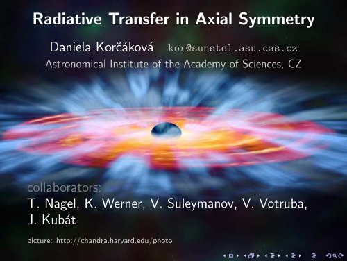
<strong>Radiative</strong> <strong>Transfer</strong> <strong>in</strong> <strong>Axial</strong> <strong>Symmetry</strong><br />
Daniela Korčáková<br />
kor@sunstel.asu.cas.cz<br />
Astronomical Institute of the Academy of Sciences, CZ<br />
collaborators:<br />
T. Nagel, K. Werner, V. Suleymanov, V. Votruba,<br />
J. Kubát<br />
picture: http://chandra.harvard.edu/photo
Outl<strong>in</strong>e<br />
Description of the method<br />
Method applicability<br />
limb darken<strong>in</strong>g<br />
stellar rotation<br />
stellar w<strong>in</strong>d<br />
discs
description of the method<br />
method preview<br />
– axial symmetry<br />
– LTE, NLTE<br />
– hydrogen<br />
– parallel version (<strong>in</strong> f<strong>in</strong>al test phase)<br />
– <strong>in</strong>put – n e (r, θ), T(r, θ), v(r, θ)<br />
χ(r, θ), S(r, θ)<br />
– output – l<strong>in</strong>e profile, <strong>in</strong>tensity map<br />
– Korčáková & Kubát, 2005, A&A 440, 715
asic idea<br />
– solution of the radiative transfer equation <strong>in</strong><br />
separate planes<br />
– polar coord<strong>in</strong>ates <strong>in</strong> every plane<br />
– comb<strong>in</strong>ation of the short and long<br />
characteristic methods<br />
– velocity field – Lorentz <strong>in</strong>variance of RTE
longitud<strong>in</strong>al planes<br />
whole radiation field<br />
rotation<br />
axis
upper boundary condition<br />
radial grid l<strong>in</strong>e<br />
grid circle<br />
zone
<strong>in</strong>tegration<br />
I (B) = I (A) e −∆τ (AB)<br />
+<br />
∫ ∆τ(AB)<br />
0<br />
S(t)e [−(∆τ (AB)−t)] dt<br />
S(t):<br />
– bound-bound<br />
– bound-free<br />
– free-free<br />
– Thomson<br />
scatter<strong>in</strong>g<br />
A<br />
∆s CD<br />
∆τ CD<br />
C<br />
∆τ<br />
B ∆s<br />
BC<br />
∆τ AB<br />
∆<br />
s<br />
AB<br />
BC<br />
D
velocity field<br />
d, th<br />
v = const.<br />
d−1, th−1<br />
∆v<br />
∆v<br />
v = const. v = const.<br />
d−1, th<br />
v = const.<br />
d, th+1<br />
v = const.<br />
d−1, th+1
solution <strong>in</strong> the central region<br />
C<br />
∆s BC<br />
∆τ<br />
BC<br />
A<br />
B<br />
∆τ<br />
AB<br />
∆s<br />
AB
lower boundary condition
mean <strong>in</strong>tensity<br />
rotation<br />
axis<br />
– the grid is def<strong>in</strong>ed<br />
by global<br />
properties<br />
– advantage – better<br />
description <strong>in</strong> outer<br />
regions, where the<br />
radiation field is<br />
strongly<br />
anisotropic
– disadvantage – not possible to use an area<br />
method<br />
– HEALPix (Hierarchical Equal Area isoLatitude<br />
Pixelization)<br />
Gorski, Hivon, Banday, Wandelt, Hansen, Re<strong>in</strong>ecke,<br />
Bartelmann, 2005, ApJ 622, 759<br />
http://healpix.jpl.nasa.gov/
parallelization<br />
– MPI<br />
– memory × computational time ×<br />
communication<br />
– formal solution of the radiative transfer<br />
equation is splitted <strong>in</strong>to the nodes by l<strong>in</strong>es<br />
– solution of the NLTE rate equations is<br />
distributed to the nodes by frequencies at the<br />
given po<strong>in</strong>t<br />
– <strong>in</strong> f<strong>in</strong>al test phase
advantages<br />
– a better description of the global character of<br />
the radiation field than by the short<br />
characteristic method<br />
– not so time consum<strong>in</strong>g as the long<br />
characteristic method<br />
– arbitrary velocity field<br />
disadvantages<br />
– high velocity gradients =⇒ a f<strong>in</strong>er grid<br />
– comput<strong>in</strong>g time ∼ f 2 (f – number of frequency<br />
po<strong>in</strong>ts)
method applicability<br />
– limb darken<strong>in</strong>g<br />
– stellar rotation<br />
– gravity darken<strong>in</strong>g, differential rotation<br />
– stellar w<strong>in</strong>d<br />
– optically th<strong>in</strong> + optically thick regions<br />
– polar + equatorial regions<br />
– Be, B[e] stars, . . .<br />
– discs<br />
– cataclysmic variables, protostellar discs<br />
– central object + surround<strong>in</strong>g medium<br />
– protoplanetary nebulae
limb darken<strong>in</strong>g<br />
the specific <strong>in</strong>tensity<br />
4e−05<br />
3e−05<br />
2e−05<br />
1e−05<br />
0<br />
0<br />
1<br />
x [r/R ∗ ]<br />
2<br />
3<br />
4.567e+14<br />
4.566e+14<br />
4.565e+14 ν<br />
4.564e+14
stellar rotation<br />
– rapidly rotat<strong>in</strong>g stars<br />
– gravity darken<strong>in</strong>g<br />
– differential rotation
extended rapidly rotat<strong>in</strong>g atmosphere<br />
1<br />
0.98<br />
relative flux<br />
0.96<br />
0.94<br />
0.92<br />
0.9<br />
rot−grav−dif<br />
rot+grav−dif<br />
rot−grav+dif<br />
rot+grav+dif<br />
4.56e+14 4.565e+14 4.57e+14 4.575e+14<br />
ν
stellar w<strong>in</strong>d<br />
– optically thick atmospheric regions +<br />
optically th<strong>in</strong> w<strong>in</strong>d<br />
– polar + equatorial region<br />
– static layers + fast outer region<br />
– stellar w<strong>in</strong>d + rotation<br />
– Be, B[e] stars
– Nv l<strong>in</strong>e 1242 Å<br />
Krtička, Korčáková, Kubát, 2008, ASPC 388, 191<br />
1<br />
relative flux<br />
0.9<br />
0.8<br />
0.7<br />
0.6<br />
one−component<br />
four−component<br />
1235 1240 1245 1250<br />
λ[Å]
discs<br />
– protostellar discs<br />
– cataclysmic variables =<br />
central white dwarf + transition region<br />
+ disc + hot corona<br />
– disc – optically thick or th<strong>in</strong><br />
– impossible to <strong>in</strong>clude a hot spot
technique<br />
– structure, χ and S from AcDc code<br />
Nagel et al., 2004, A&A, 428, 109<br />
– disc = set of concentric r<strong>in</strong>gs<br />
– consistent solution of:<br />
– radiative transfer equation<br />
– hydrostatic equation<br />
– energy balance equation<br />
– rate equation<br />
– equation of charge and particle conservation<br />
– 2D grid<br />
– <strong>in</strong>terpolation of S and χ to the new grid<br />
Steffen, 1990, A&A, 239, 443<br />
– Kepler rotation law<br />
– radiative transfer us<strong>in</strong>g the 2.5D code
choice of the systems<br />
– the quiescent phase – optically th<strong>in</strong>ner =⇒<br />
effects connected with the velocity field better<br />
visible<br />
– SS Cyg<br />
– Hα<br />
– Hγ<br />
– an AM CVn system<br />
– HeI 4923 Å
SS Cyg<br />
– an <strong>in</strong>termediate polar<br />
M ∗ wd<br />
(0.81 ± 0.19)M ⊙<br />
q ∗ = M K /M wd 0.683 ± 0.012<br />
a ∗<br />
R ∗∗<br />
wd<br />
P ∗<br />
i ∗<br />
(1.36 ± 0.11) × 10 11 cm<br />
0.011R ⊙<br />
0.27512973 days<br />
45 ◦ − 56 ◦<br />
∗ Bitner et al., 2007, ApJ, 662, 564<br />
∗∗ Wood, 1995, LNP, 443, 41<br />
– model – H + He – 8 r<strong>in</strong>gs;<br />
Ṁ∈< 1 × 10 −11 , 1 × 10 −9 > M ⊙ yr −1
SS Cyg – quiescent phase – Hα<br />
y [R wd ]<br />
5<br />
4<br />
3<br />
2<br />
log(χ )<br />
-2 0<br />
-4<br />
-6<br />
-8<br />
-10<br />
-12<br />
-14<br />
-16<br />
-18<br />
1<br />
0<br />
5<br />
0 10 20 30 40 50 60 r tidal<br />
x [R wd ] 4<br />
y [R wd ]<br />
3<br />
2<br />
log(S)<br />
-2<br />
-3<br />
-4<br />
-5<br />
-6<br />
-7<br />
-8<br />
-9<br />
1<br />
0<br />
0 10 20 30 40 50 60<br />
x [R wd ]<br />
r tidal
SS Cyg – quiescent phase – Hα<br />
relative flux<br />
2.8<br />
2.6<br />
2.4<br />
2.2<br />
2<br />
1.8<br />
1.6<br />
1.4<br />
1.2<br />
1<br />
i=0 o RTE<br />
flux<br />
relative flux<br />
1.04<br />
1.03<br />
1.02<br />
1.01<br />
1<br />
i=85 o RTE<br />
flux<br />
4.55e+14 4.6e+14<br />
ν[Hz]<br />
4.55e+14 4.6e+14<br />
ν[Hz]<br />
relative flux<br />
1.15<br />
1.1<br />
1.05<br />
i=70 o RTE<br />
flux<br />
relative flux<br />
1.15<br />
1.1<br />
1.05<br />
i=90 o RTE<br />
flux<br />
1<br />
1<br />
4.55e+14 4.6e+14<br />
ν[Hz]<br />
4.55e+14 4.6e+14<br />
ν[Hz]
SS Cyg – quiescent phase – Hγ<br />
y [R wd ]<br />
5<br />
4<br />
3<br />
2<br />
log(χ )<br />
-2<br />
-4<br />
-6<br />
-8<br />
-10<br />
-12<br />
-14<br />
-16<br />
1<br />
0<br />
5<br />
0 10 20 30 40 50 60 r tidal<br />
x [R wd ] 4<br />
y [R wd ]<br />
3<br />
2<br />
log(S)<br />
-2<br />
-3<br />
-4<br />
-5<br />
-6<br />
-7<br />
-8<br />
-9<br />
1<br />
0<br />
0 10 20 30 40 50 60<br />
x [R wd ]<br />
r tidal
SS Cyg – quiescent phase – Hγ<br />
2<br />
1.04<br />
relative flux<br />
1.8<br />
1.6<br />
1.4<br />
1.2<br />
i=0 o RTE<br />
flux<br />
relative flux<br />
1.03<br />
1.02<br />
1.01<br />
i=85.0 o<br />
RTE<br />
flux<br />
1<br />
6.85e+14 6.9e+14 6.95e+14<br />
ν[Hz]<br />
1<br />
6.85e+14 6.9e+14 6.95e+14<br />
ν[Hz]<br />
relative flux<br />
1.08<br />
1.06<br />
1.04<br />
1.02<br />
i=70 o RTE<br />
flux<br />
relative flux<br />
1.1<br />
1.05<br />
1<br />
i=90 o RTE<br />
flux<br />
1<br />
6.85e+14 6.9e+14 6.95e+14<br />
ν[Hz]<br />
0.95<br />
6.85e+14 6.9e+14 6.95e+14<br />
ν[Hz]
an AM CVn star<br />
– P orb < 1 hour =⇒ compact donors<br />
– nature<br />
– white dwarf (neutron star) + white dwarf<br />
– white dwarf (neutron star) + helium core burn<strong>in</strong>g<br />
star<br />
– white dwarf (neutron star) + ma<strong>in</strong>-sequence star<br />
– model (GP Com)<br />
– quiescence phase<br />
– 9 r<strong>in</strong>gs<br />
– Ṁ∼ 10 −11 M ⊙ yr −1<br />
– HeI 4923Å
an AM CVn star – HeI 4923Å<br />
y [R wd ]<br />
0.15<br />
0.1<br />
0.05<br />
log(χ )<br />
-2<br />
-4<br />
-6<br />
-8<br />
-10<br />
-12<br />
-14<br />
-16<br />
-18<br />
0.15<br />
0<br />
0 2 4 6 8 10 12<br />
x [R 0.1<br />
wd ]<br />
0.05<br />
y [R wd ]<br />
log(S)<br />
-2<br />
-3<br />
-4<br />
-5<br />
-6<br />
-7<br />
-8<br />
-9<br />
0<br />
0 2 4 6 8 10 12<br />
x [R wd ]
an AM CVn star – HeI 4923Å<br />
relative flux<br />
31<br />
21<br />
11<br />
i=0 o RTE<br />
flux<br />
relative flux<br />
1.3<br />
1.2<br />
1.1<br />
i=89.0 o<br />
RTE<br />
flux<br />
1<br />
6.05e+14 6.1e+14 6.15e+14<br />
ν[Hz]<br />
1<br />
6.05e+14 6.1e+14 6.15e+14<br />
ν[Hz]<br />
1.6<br />
2.2<br />
relative flux<br />
1.5<br />
1.4<br />
1.3<br />
1.2<br />
1.1<br />
1<br />
i=70 o RTE<br />
flux<br />
6.05e+14 6.1e+14 6.15e+14<br />
ν[Hz]<br />
relative flux<br />
2<br />
1.8<br />
1.6<br />
1.4<br />
1.2<br />
1<br />
i=90 o RTE<br />
flux<br />
6.05e+14 6.1e+14 6.15e+14<br />
ν[Hz]
– face-on view<br />
– rotation velocity field has a negligible <strong>in</strong>fluence<br />
– static disc approximation for the radiative transfer<br />
is valid with high accuracy<br />
– edge-on view<br />
– important difference<br />
v rot [km/s]<br />
y [R wd ]<br />
5<br />
4<br />
3<br />
2<br />
2500<br />
2000<br />
1500<br />
1000<br />
500<br />
0<br />
1<br />
0<br />
0 10 20 30 40 50 60<br />
x [R wd ]<br />
r tidal
Where it can play the role?<br />
– edge-on view – open<strong>in</strong>g angle ∼ 10 ◦<br />
– not so small probability<br />
– self-shield<strong>in</strong>g disc (e.g. V348 Pup)<br />
– occult<strong>in</strong>g systems – some UX UMa or SW Ser<br />
systems<br />
– low lum<strong>in</strong>osity<br />
– dust is not important <strong>in</strong> most CVs (<strong>in</strong> contrast to<br />
polars)<br />
– extended area<br />
– w<strong>in</strong>d<br />
– important corona – polars, <strong>in</strong>termediate polars
conclusion<br />
– axial symmetry + w<strong>in</strong>d + rotation =⇒<br />
– rapidly rotat<strong>in</strong>g stars<br />
– extended stellar atmospheres<br />
– stellar w<strong>in</strong>ds<br />
– discs