THESE de DOCTORAT - cerfacs
THESE de DOCTORAT - cerfacs THESE de DOCTORAT - cerfacs
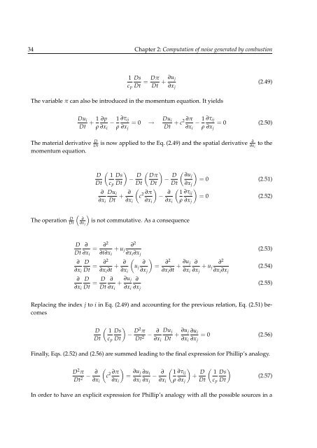
34 Chapter 2: Computation of noise generated by combustion 1 Ds c p Dt = Dπ Dt + ∂u j (2.49) ∂x j The variable π can also be introduced in the momentum equation. It yields Du i Dt + 1 ∂p − 1 ∂τ ij = 0 → Du i ∂π + c2 − 1 ∂τ ij = 0 (2.50) ρ ∂x i ρ ∂x j Dt ∂x i ρ ∂x j The material derivative D Dt momentum equation. is now applied to the Eq. (2.49) and the spatial derivative ∂ ∂x i to the D Dt ( ) 1 Ds − D c p Dt Dt ( ) Dπ − D ( ) ∂uj = 0 (2.51) Dt Dt ∂x j ∂ Du i ∂x i Dt + ∂ ( c 2 ∂π ) − ∂ ( ) 1 ∂τ ij = 0 (2.52) ∂x i ∂x i ∂x i ρ ∂x j The operation D Dt ( ∂ ∂x j ) is not commutative. As a consequence D Dt ∂ ∂x i = ∂ D ∂x i Dt = ∂ ∂x i D Dt = D Dt ∂2 ∂ + 2 u j (2.53) ∂t∂x i ∂x i ∂x j ∂2 ∂x i ∂t + ∂ ( ) ∂ u j = ∂2 ∂x i ∂x j ∂x i ∂t + ∂u j ∂ ∂ + 2 u j (2.54) ∂x i ∂x j ∂x i ∂x j ∂ ∂x i + ∂u j ∂x i ∂ ∂x j (2.55) Replacing the index j to i in Eq. (2.49) and accounting for the previous relation, Eq. (2.51) becomes D Dt ( ) 1 Ds − D2 π c p Dt Dt 2 − ∂ Du j ∂x i Dt + ∂u j ∂u i = 0 (2.56) ∂x i ∂x j Finally, Eqs. (2.52) and (2.56) are summed leading to the final expression for Phillip’s analogy. D 2 π Dt 2 − ∂ ( c 2 ∂π ) = ∂u j ∂u i − ∂ ( ) 1 ∂τ ij + D ∂x i ∂x i ∂x i ∂x j ∂x i ρ ∂x j Dt ( ) 1 Ds c p Dt (2.57) In order to have an explicit expression for Phillip’s analogy with all the possible sources in a
2.3 Hybrid computation of noise: Acoustic Analogies 35 reacting flow, the energy equation Eq. (2.28) is combined with Eq. (2.47) leading to [ 1 Ds (γ − 1) = c p Dt ρc 2 Phillip’s equation for reacting flows reads D 2 π Dt 2 − ∂ ( c 2 ∂π ) = ∂u j ∂u i − ∂ ∂x i ∂x i ∂x i ∂x j + D Dt ] ∂J ˙ω T + ∑ h k k − ∂q i + τ ij : ∂u i + ˙Q + D (ln r) (2.58) ∂x k i ∂x i ∂x j Dt ∂x i ( 1 ρ [ ( (γ − 1) ρc 2 ) ∂τ ij ∂x j ∂J ˙ω T + ∑ h k k − ∂q i + τ ij : ∂u i + ˙Q (2.59) ∂x k i ∂x i ∂x j Dt 2 (ln r) + D2 Equation (2.59) was introduced by Chiu & Summerfield [14] and Kotake [39]. This expression accounts for some acoustic-flow interactions, since gradients of the sound velocity c are included in the acoustic operator. It has several advantages compared to Lighthill’s analogy, since mean temperature and density of the propagation medium are not assumed homogeneous in space, which is clearly the case for reacting flows. The term responsible for noise generation due to hydrodynamic fluctuations is now defined as ∂u j ∂x i ∂u i ∂x j . The density contribution in this term has been removed, contrary to its form in Lighthill’s analogy ∂2 ∂x i ∂x j (ρu i u j ). It is clear then that for low Mach numbers there is not anymore ambiguity in this source definition since acoustic-flow interactions are not anymore included in this term [4]. Nevertheless, Lilley [52] demonstrated that when the Mach number is not negligible, acoustic-flow interactions are still contained in the compressible part of u i . Another interesting remark done by Bailly [4] is that in this equation the source responsible for indirect noise (the acceleration of density inhomogeneities) no longer appears. It is recommended therefore that if indirect noise is not negligible and no strong changes in the mean flow are present, Lighthill’s analogy should be the formulation under consideration. )] Simplifying Phillips’ Analogy Phillips’ equation (Eq. 2.59), as Lighthill’s formulation, is an exact rearrangement of the fluid dynamics equations. Similar assumptions as those made in section 2.3.2 are considered here. It is assumed then that the diffusion of species J k , the dissipation function τ ∂u i ∂x j , external energy sources ˙Q, heat fluxes ∂q i ∂x i , the viscosity stresses τ ij , changes in the molecular weight of the mixture D Dt (ln r) and the Reynolds stress tensor ρu iu j are neglected in comparison to the monopolar source of noise ∂ ˙ω T ∂t . The simplified Phillips’ equation then reads:
- Page 1: UNIVERSITE MONTPELLIER II SCIENCES
- Page 5: An expert is a man who has made all
- Page 8 and 9: Y gracias familia mía!!, que así
- Page 11: Abstract Today, much of the current
- Page 14 and 15: 4 CONTENTS 3.4.1 Preconditioning .
- Page 16 and 17: List of Figures 1.1 Main sources of
- Page 18 and 19: 8 LIST OF FIGURES 5.19 Acoustic ene
- Page 20: List of Tables 1.1 EU recommended r
- Page 24 and 25: 14 Chapter 1: General Introduction
- Page 26 and 27: 16 Chapter 1: General Introduction
- Page 28 and 29: 18 Chapter 1: General Introduction
- Page 30 and 31: 2 Computation of noise generated by
- Page 32 and 33: 22 Chapter 2: Computation of noise
- Page 34 and 35: 24 Chapter 2: Computation of noise
- Page 36 and 37: 26 Chapter 2: Computation of noise
- Page 38 and 39: 28 Chapter 2: Computation of noise
- Page 40 and 41: 30 Chapter 2: Computation of noise
- Page 42 and 43: 32 Chapter 2: Computation of noise
- Page 46 and 47: 36 Chapter 2: Computation of noise
- Page 48 and 49: 38 Chapter 2: Computation of noise
- Page 50 and 51: 40 Chapter 2: Computation of noise
- Page 52 and 53: 42 Chapter 3: Development of a nume
- Page 54 and 55: 44 Chapter 3: Development of a nume
- Page 56 and 57: 46 Chapter 3: Development of a nume
- Page 58 and 59: 48 Chapter 3: Development of a nume
- Page 60 and 61: 50 Chapter 3: Development of a nume
- Page 62 and 63: 52 Chapter 3: Development of a nume
- Page 64 and 65: 54 Chapter 3: Development of a nume
- Page 66 and 67: 56 Chapter 3: Development of a nume
- Page 68 and 69: 4 Validation of the acoustic code A
- Page 70 and 71: 60 Chapter 4: Validation of the aco
- Page 72 and 73: 62 Chapter 4: Validation of the aco
- Page 74 and 75: 64 Chapter 4: Validation of the aco
- Page 76 and 77: 66 Chapter 4: Validation of the aco
- Page 78 and 79: 68 Chapter 4: Validation of the aco
- Page 80 and 81: 70 Chapter 4: Validation of the aco
- Page 82 and 83: 5 Assessment of combustion noise in
- Page 84 and 85: 74 Chapter 5: Assessment of combust
- Page 86 and 87: 76 Chapter 5: Assessment of combust
- Page 88 and 89: 78 Chapter 5: Assessment of combust
- Page 90 and 91: 80 Chapter 5: Assessment of combust
- Page 92 and 93: 82 Chapter 5: Assessment of combust
34 Chapter 2: Computation of noise generated by combustion<br />
1 Ds<br />
c p Dt = Dπ<br />
Dt + ∂u j<br />
(2.49)<br />
∂x j<br />
The variable π can also be introduced in the momentum equation. It yields<br />
Du i<br />
Dt + 1 ∂p<br />
− 1 ∂τ ij<br />
= 0 → Du i ∂π<br />
+ c2 − 1 ∂τ ij<br />
= 0 (2.50)<br />
ρ ∂x i ρ ∂x j Dt ∂x i ρ ∂x j<br />
The material <strong>de</strong>rivative D Dt<br />
momentum equation.<br />
is now applied to the Eq. (2.49) and the spatial <strong>de</strong>rivative<br />
∂<br />
∂x i<br />
to the<br />
D<br />
Dt<br />
( ) 1 Ds<br />
− D c p Dt Dt<br />
( ) Dπ<br />
− D ( ) ∂uj<br />
= 0 (2.51)<br />
Dt Dt ∂x j<br />
∂ Du i<br />
∂x i Dt + ∂ (<br />
c 2 ∂π )<br />
− ∂ ( ) 1 ∂τ ij<br />
= 0 (2.52)<br />
∂x i ∂x i ∂x i ρ ∂x j<br />
The operation D Dt<br />
(<br />
∂<br />
∂x j<br />
)<br />
is not commutative. As a consequence<br />
D<br />
Dt<br />
∂<br />
∂x i<br />
=<br />
∂ D<br />
∂x i Dt =<br />
∂<br />
∂x i<br />
D<br />
Dt = D Dt<br />
∂2 ∂<br />
+ 2<br />
u j (2.53)<br />
∂t∂x i ∂x i ∂x j ∂2<br />
∂x i ∂t + ∂ ( )<br />
∂<br />
u j = ∂2<br />
∂x i ∂x j ∂x i ∂t + ∂u j ∂ ∂<br />
+ 2<br />
u j (2.54)<br />
∂x i ∂x j ∂x i ∂x j<br />
∂<br />
∂x i<br />
+ ∂u j<br />
∂x i<br />
∂<br />
∂x j<br />
(2.55)<br />
Replacing the in<strong>de</strong>x j to i in Eq. (2.49) and accounting for the previous relation, Eq. (2.51) becomes<br />
D<br />
Dt<br />
( ) 1 Ds<br />
− D2 π<br />
c p Dt Dt 2 − ∂ Du j<br />
∂x i Dt + ∂u j ∂u i<br />
= 0 (2.56)<br />
∂x i ∂x j<br />
Finally, Eqs. (2.52) and (2.56) are summed leading to the final expression for Phillip’s analogy.<br />
D 2 π<br />
Dt 2 − ∂ (<br />
c 2 ∂π )<br />
= ∂u j ∂u i<br />
− ∂ ( ) 1 ∂τ ij<br />
+ D ∂x i ∂x i ∂x i ∂x j ∂x i ρ ∂x j Dt<br />
( ) 1 Ds<br />
c p Dt<br />
(2.57)<br />
In or<strong>de</strong>r to have an explicit expression for Phillip’s analogy with all the possible sources in a


