Continuous Wavelet Transform on the Hyperboloid - Université de ...

<strong>Continuous</strong> <strong>Wavelet</strong> <strong>Transform</strong> on the
Hyperboloid
Iva Bogdanova 1 , Pierre Vandergheynst 1
École Polytechnique Fédérale de Lausanne (EPFL), Signal Processing Institute,
CH-1015 Lausanne, Switzerland
Jean-Pierre Gazeau 2
Laboratory of Astroparticle and Cosmology, Université Paris 7 - Denis Diderot,
75251 Paris cedex 05, France
Abstract
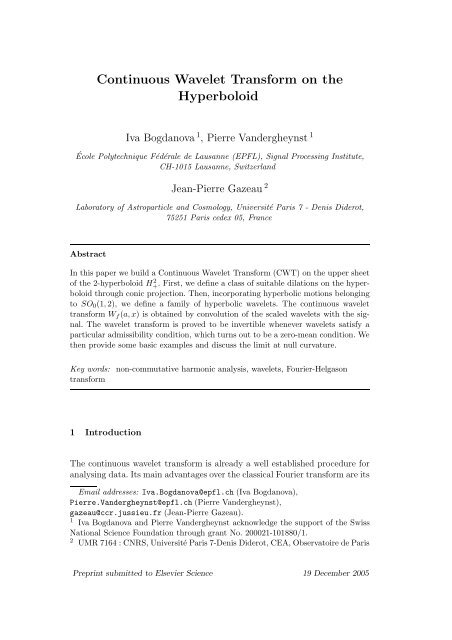
In this paper we build a <strong>Continuous</strong> <strong>Wavelet</strong> <strong>Transform</strong> (CWT) on the upper sheet
of the 2-hyperboloid H+ 2 . First, we define a class of suitable dilations on the hyperboloid
through conic projection. Then, incorporating hyperbolic motions belonging
to SO 0 (1, 2), we define a family of hyperbolic wavelets. The continuous wavelet
transform W f (a, x) is obtained by convolution of the scaled wavelets with the signal.
The wavelet transform is proved to be invertible whenever wavelets satisfy a
particular admissibility condition, which turns out to be a zero-mean condition. We
then provide some basic examples and discuss the limit at null curvature.
Key words: non-commutative harmonic analysis, wavelets, Fourier-Helgason
transform
1 Introduction
The continuous wavelet transform is already a well established procedure for
analysing data. Its main advantages over the classical Fourier transform are its
Email addresses: Iva.Bogdanova@epfl.ch (Iva Bogdanova),
Pierre.Vandergheynst@epfl.ch (Pierre Vandergheynst),
gazeau@ccr.jussieu.fr (Jean-Pierre Gazeau).
1 Iva Bogdanova and Pierre Vandergheynst acknowledge the support of the Swiss
National Science Foundation through grant No. 200021-101880/1.
2 UMR 7164 : CNRS, Université Paris 7-Denis Diderot, CEA, Observatoire de Paris
Preprint submitted to Elsevier Science 19 December 2005

local and multiresolution nature, which provide the interesting properties of
a mathematical microscope. Its theory is well known in the case of the line or
other higher dimensional Euclidean spaces [Antoine et al., 2005, Mallat, 1998]
and the wavelet transform has certainly become a standard in data analysis.
However, data analysis has undergone deep changes recently and the field faces
new exciting challenges. On one hand the volume of data is exploding due to
the ubiquity of digital sensors (just think of digital cameras). The first challenge
resides in extracting information from very high dimensional data. On
the other hand, the type of data has also evolved tremendously over the past
few decade, from images or volumetric data to non-scalar valued signals. One
can cite for example tensor diffusion imaging, a new modality in medical imaging
[Hagmann et al., 2003], or multimodal signals, i.e signals obtained when
the same physical scene is observed through different sensors. Finally, there
are instances where data are collected on a surface, or more generally a manifold,
or through a complicated interface (think of the human eye for example).
This is often the case in astrophysics and cosmology [Martinez-Gonzalez et al.,
2002, Cayon et al., 2003], geophysics but also in neurosciences [Angenent et al.,
1999], computational chemistry [Max and Getzoff, 1988] ... The list is truly
endless. The second challenge thus resides in the complexity of data sources
and a field one could call Complex Data Processing might be emerging.
A given feature shared by all these problems is the importance of geometry :
either important information is localized around highly structured submanifolds,
or data types obey intrinsic nonlinear constraints. As a consequence of
the challenges in complex data processing, the representation and analysis of
signals in non-Euclidean geometry is now a recurrent problem in many scientific
domains. Because of these demands, spherical wavelets [Antoine and
Vandergheynst, 1999] were recently developed and applied in various fields,
from Cosmology [McEwen et al., 2004] to Computer Vision [Tosic et al., 2005].
Although the sphere is a manifold most desirable for applications, the mathematicalanalysismadesofarinvitesusto
consider other manifolds with similar
geometrical properties, and first of all, other Riemannian symmetric spaces of
constant curvature. Among them, the two-sheeted hyperboloid H 2 stands as a
very interesting case. For instance, such a manifold may be viewed as the phase
space for the motion of a free particle in 1+1-anti de Sitter spacetime [Gazeau
et al., 1989, Gazeau and Hussin, 1992]. Other examples come from physical
systems constrained on a hyperbolic manifold, for instance, an open expanding
model of the universe. A completely different example of application is
provided by the emerging field of catadioptric image processing [Makadia and
Daniilidis, 2003, Daniilidis et al., 2002]. In this case, a normal (flat) sensor is
overlooking a curved mirror in order to obtain an omnidirectional picture of
the physical scene. An efficient system is obtained using a hyperbolic mirror,
since it has a single effective viewpoint. Finally, from a purely conceptual point
of view, having already built the CWT for data analysis in Euclidean spaces
2

and on the sphere, it is natural to raise the question of its existence and form
on the dual manifold.
In general, for constructing a CWT on H 2 , few basic requirements should be
satisfied
• wavelets and signals must “live” on the hyperboloid;
• the transform must involve dilations of some kind; and
• the CWT on H 2 should reduce locally to the usual CWT on the plane.
The paper is organized as follows. In Section 2 we sketch the geometry of
the two-sheeted hyperboloid H 2 . In Section 3 we define affine transformations
on the upper sheet H+ 2 of H2 . There are two fundamental operations : dilations
and hyperbolic motions represented by the group SO 0 (1, 2). Then, the
action of the dilation on the hyperboloid is derived in Section 4. In Section 5,
harmonic analysis on the hyperboloid is introduced by means of the Fourier-
Helgason transform : this is a central tool for constructing and studying the
wavelet transform. Section 6 really constitutes the core of this paper. First
we define the CWT on H+ 2 through a hyperbolic convolution. Then we prove
a hyperbolic version of the Fourier convolution theorem which allows us to
work conveniently in the Fourier-Helgason domain. Theorems 4 and 5 are our
main results. We would like to state them roughly here in order to wet our
readers’ appetite since these results are reminiscent of their Euclidean counterparts.
The first one states a generic admissibility condition for the existence
of hyperbolic wavelets :
Featured Theorem 1 (Admissible wavelets) Let ψ be a compactly supported,
square integrable, continuous function on H+ 2 whose Fourier-Helgason
coefficients satisfy :
0 < A ψ (ν) =
∫ ∞
0
| ̂ψ a (ν)| 2 α(a)da2, then the following zero-mean
condition has to be satisfied :
A square integrable function on H 2 + with bounded support is a wavelet if its
3

x
0
H 2 +
x
2
x
1
Fig. 1. Geometry of the 2-hyperboloid.
integral vanishes when it is conveniently weighted, that is
for p>0.
∫
H 2 +
dµ(χ, ϕ)
[ ] 1
sinh 2pχ
2
ψ(χ, ϕ) =0,
sinh χ
Finally we conclude this paper with illustrating examples of hyperbolic wavelets
and wavelet transforms and give directions for future work.
2 Geometry of the two-sheeted hyperboloid. Projective structures.
We start by recalling basic facts about the upper sheet of the two-sheeted
hyperboloid of radius ρ, H 2 +ρ. Letχ, ϕ be a system of polar coordinates for
H 2 +ρ . To each point θ =(χ, ϕ) we shall associate the vector x =(x 0,x 1 ,x 2 )of
R 3 given by
x 0 = ρ cosh χ,
x 1 = ρ sinh χ cos ϕ, ρ > 0, χ 0, 0 ≤ ϕ

0
x
0
C 2 +
H 2 +
r
0
x
2
x
1
Fig. 2. Cross-section of a conic projection
called Lobachevskian metric, whereas the measure element on the hyperboloid
is
dµ = ρ 2 sinh χdχdϕ. (2)
In the sequel, we shall put ρ = 1 for convenience and designate the unit
hyperboloid H 2 +ρ=1 by H 2 +.
Various projections can be used to endow H+ 2 with a local Euclidean structure.
One of them is immediate : it suffices to flatten the hyperboloid onto R 2 ≃ C.
Another possibility is to project the hyperboloid onto a cone. Let us consider
a half null cone C+ 2 ∈ R 3 of equation (x 0 ) 2 − 1
tan ψ 0
((x 1 ) 2 +(x 2 ) 2 )=0,x 0 0.
This cone C+ 2 has Euclidean nature. The cone surface unrolled is a circular
sector and all points of H+ 2 will be mapped onto C+ 2 using a specific conic
projection. The characteristic parameter of a conic projection is the constant
of the cone m =cosψ 0 ,whereψ 0 is the Euclidean angle of inclination of the
generatrix of the cone as shown in Figure 2.
Considering a radial conic projection, it is more convenient to use a radius r
defined by the Euclidean distance between a point on the cone, conic projection
of the point (χ, ϕ) ∈ H 2 + ,andthex 0-axis:
r = f(χ), dr = f ′ (χ)dχ with
dr
=1. (3)
dχ∣ χ=0
Each suitable projection is determined by a specific choice of f(χ). It is clear
that dilation of the cone C 2 + ↦→ aC 2 + = C 2 + entails r ↦→ ar. Consequently, the
resulting map χ ↦→ χ a is determined by f(χ a )=af(χ). This is precisely the
point at the heart of our approach and we shall discuss this more precisely in
Section 4.
5

3 Affine transformations on the 2-hyperboloid
We recall that our purpose is to build a total family of functions in L 2 (H 2 +, dµ)
by picking a wavelet or probe ψ(χ) with suitable localization properties and
applying on it hyperbolic motions, belonging to the group SO 0 (1, 2), supplemented
by appropriate dilations
ψ(x) → λ(a, x)ψ(d 1/a g −1 x) ≡ ψ a,g (x), g ∈ SO 0 (1, 2), a∈ R + ∗ . (4)
Dilations d a will be studied below. Hyperbolic rotations and motions, g ∈
SO 0 (1, 2), act on x in the following way.
Amotiong ∈ SO 0 (1, 2) can be factorized as g = k 1 hk 2 ,wherek 1 ,k 2 ∈
SO(2), h∈ SO 0 (1, 1), and the respective action of k and h are the following
⎛
⎞ ⎛
⎞
1 0 0
cosh χ
k(ϕ 0 ).x(χ, ϕ)=
⎜ 0cosϕ 0 − sin ϕ 0
⎟ ⎜ sinh χ cos ϕ
⎟
⎝
⎠ ⎝
⎠
0sinϕ 0 cos ϕ 0 sinh χ sin ϕ
= x(χ, ϕ + ϕ 0 ), (6)
⎛
⎞ ⎛
⎞
cosh χ 0 sinh χ 0 0
cosh χ
h(χ 0 ).x(χ, ϕ)=
⎜ sinh χ 0 cosh χ 0 0
⎟ ⎜ sinh χ cos ϕ
(7)
⎟
⎝
⎠ ⎝
⎠
0 0 1 sinh χ sin ϕ
= x(χ + χ 0 ,ϕ) . (8)
(5)
On the other hand, the dilation is a homeomorphism d a : H 2 + → H 2 + and we
require that d a fulfills the two conditions:
(i) it monotonically dilates the azimuthal distance between two points on H 2 +:
where dist(x, x ′ ) is defined by
dist(d a (x), d a (x ′ )), (9)
dist(x, x ′ )=cosh −1 (x · x ′ ), (10)
and the dot product is the Minkowski product in R 3 ;notethatdist(x, x ′ )
reduces to |χ − χ ′ | when ϕ = ϕ ′ ;
(ii) it is homomorphic to the group R + ∗ ;
R + ∗ ∋ a → d a , d ab = d a d b , d a −1 = d −1
a , d 1 = I d .
6

The action of a motion on a point x ∈ H+ 2 is trivial: it displaces (rotates) by
a hyperbolic angle χ ∈ R + (respectively by an angle ϕ). It has to be noted
that, as opposed to the case of the sphere, attempting to use the conformal
group SO 0 (1, 3) for describing dilation, our requirements are not satisfied.
In particular, conformal dilations do not preserve the upper sheet H+ 2 of the
hyperboloid. In this paper we adopt an alternative procedure that describes
different maps for dilating the hyperboloid.
4 Dilations on hyperboloid
Considering the half null-cone of equation
{
}
C+ 2 = ξ ∈ R 3 : ξ · ξ = ξ0 2 − ξ1 2 − ξ2 2 =0, ξ 0 > 0 , (11)
there exist the SO 0 (1, 2)-motions and the obvious Euclidean dilations
ξ ∈ C 2 + → aξ ∈ C2 + ≡ dC2 +
a (ξ), (12)
which form a multiplicative one-parameter group isomorphic to R + ∗ .
In order to lift dilation (12) back to H+ 2 , it is natural to use possible conic
projections of H+ 2 onto C2 + , as defined in Section 2.
H 2 + ∋ x → Φ(x) ∈ C2 + → Π 0Φ(x) ∈ R 2 ≃ C, (13)
where Π 0 stands for flattening, defined by
Π 0 Φ(x) :x(r, ϕ) ∈ C 2 + ↦→ reiϕ ∈ C. (14)
Flattening reveals the Euclidean nature of the conic projection and the full
action of (14) is depicted on Figure 3. Then, we might wish to find a form of
Π 0 Φ such that, expressed in polar coordinates, the measure is
dµ = rdrdϕ. (15)
In this case, dilating r will quadratically dilate the measure dµ as well. By
expressing the measure (15) with the radius defined in (3) we obtain
f(χ)f ′ (χ) =sinhχ =⇒ f(χ) =2sinh χ 2 . (16)
Consequently, the radius of this particular conic projection is r =2sinh χ 2 .
7

x
0
H 2 +
N
P
P
P
P
0
x
1
C
x
2
Fig. 3. Conic projection and flattening.
Thus, this conic projection Φ : H+ 2 → C2 + is a bijection given, after flattening,
by
Π 0 Φ(x) =2sinh χ 2 eiϕ ,
with x ≡ (χ, ϕ), χ ∈ R + , 0 ≤ ϕ

4
p=0.5
4
p=1
3.5
3.5
3
3
2.5
2.5
2
2
1.5
1.5
1
1
0.5
0.5
0
−4 −3 −2 −1 0 1 2 3 4
0
−4 −3 −2 −1 0 1 2 3 4
Fig. 4. Cross-section of conic projections for different values of parameter p.
x
0
H 2 +
a
P
P a
N
P
P
x
1
C
0
P
P
Pa
P
0
x
2
Fig. 5. Action of a dilation a on the hyperboloid H 2 + by conic projection with
parameter p =1.
The action of dilation by conic projection is given by
sinh pχ a = a sinh pχ (21)
The particular case p = 1 is depicted in Figure 5. The dilated point x a ∈ H+
2
is
x a =(coshχ a , sinh χ a cos ϕ, sinh χ a sin ϕ), (22)
with polar coordinates θ a =(χ a ,ϕ). The behaviour of dist(x N , x a ), with x N
being the North Pole, is shown in Figure 6 in the case p =0.1, p =0.5 and
p = 1. We can see that this is an increasing function with respect to the
dilation a.
It is also interesting to compute the action of dilations in the bounded version
of H+ 2 . The latter is obtained by applying the stereographic projection from
the South Pole of H 2 and it maps the upper sheet H+ 2 onto the open unit disc
9

2
1.8
1.6
p=0.1
p=0.5
p=1
1.4
dist(x N
, x a
)
1.2
1
0.8
0.6
0.4
0.2
0
0 0.5 1 1.5 2 2.5 3
dilation a
Fig. 6. Analysis of the distance (9) as a function of dilation a, withx N being the
North Pole and using conic projection for different parameter p.
in the equatorial plane:
x = x(χ, ϕ) → Φ(x) =tanh χ 2 eiϕ . (23)
In the case p = 1 2
by using (17) and basic trigonometric relations, we obtain
tanh χ a
2 = √ √√√
a 2 tanh 2 χ 2
1+(a 2 − 1) tanh 2 χ 2
≡ ζ. (24)
In this case, the dilation leaves invariant both ζ =0andζ = 1, the center
and the border of the disc, respectively. Figure 7 depicts the action of this
transformation on a point x ∈ H+ 2 . A dilation from the North Pole (D N)is
considered as a dilation in the unit disc in equatorial plane and lifted back
to H+ 2 by inverse stereographic projection from the South Pole. A dilation
from any other point x ∈ H+ 2 is obtained by moving x to the North Pole by
a rotation g ∈ SO 0 (1, 2), performing dilation D N and going back by inverse
rotation:
D x = g −1 D N g.
The visualization of the dilation on the hyperboloid H+ 2 ,withp = 0.5, is
provided in Figure 8. There, each circle represents points on the hyperboloid
at constant χ and is dilated by the scale factor a =0.75.
10

x
0
H 2 +
a
N
x
1
a
S
x
2
H 2 -
Fig. 7. Action of a dilation a on the hyperboloid H 2 + through a stereographic projection
(case p = 1 2 ).
Fig. 8. Visualization of the dilation on the hyperboloid H 2 + (case p = 1 2 ).
5 Harmonic analysis on the 2-hyperboloid
5.1 Fourier-Helgason <strong>Transform</strong>
This integral transform is the precise analog of the Fourier-Plancherel transform
on R n . It consists of an isometry between two Hilbert spaces
FH : L 2 (H 2 +, dµ) −→ L 2 (L, dη), (25)
11

where the measure dµ is the SO 0 (1, 2)-invariant measure on H 2 + and L2 (L, dη)
denotes the Hilbert space of sections of a line-bundle L over another suitably
defined manifold, the so-called Helgason-dual of H 2 + and denoted by Ξ. We
note here that R n is its own Helgason-dual.
Let us see what is the concrete realization of the dual space Ξ. Most of the
following discussion can be found in [Ali and Bertola, 2002], and we summarize
it here for convenience. In fact Ξ can be realized as the projective half nullcone,
as defined in (11) and asymptotic to H+ 2 , times the positive real line.
The space Ξ is given by
Ξ=R + × PC + ≡{k =(ν, ⃗ ξ)}, (26)
where PC + denotes the projective forward cone {ξ ∈ C 2 + | λξ ≡ ξ, λ >
0, ξ 0 > 0} (the set of “rays” on the cone). A convenient realization of PC +
makes it diffeomorphic to the 1-sphere S 1 as follows
PC + ≃{ ⃗ ξ ∈ R 2 : ‖ ⃗ ξ‖ =1}∼S 1 (27)
ξ ≡ (ξ 0 , ⃗ ξ)=(ξ 0 ,ξ 1 ,ξ 2 ) ↦→ 1 ξ 0
⃗ ξ. (28)
The Fourier - Helgason transform is defined in a way similar to the ordinary
Fourier transform by using the eigenfunctions of the invariant differential operator
of second order, i.e. the Laplacian on H+ 2 . In our case, the functions of
the (unique) invariant differential operator are named hyperbolic plane waves
[Bros et al., 1994]
E ν,ξ (x) =(ξ · x) − 1 2 −iν , ν ∈ R + ,ξ∈ C 2 +. (29)
These waves are not parametrized by points of R + ×PC + but rather by points
of R + × C+; 2 however the action of R + on C+ 2 just rescales them by a factor
which is constant in x ∈ H+ 2 . In other words, they are sections of an appropriate
line-bundle over Ξ, which we denote by L, andC+ 2 is thought of as total
space of R + over PC + . As well, we note that the inner product ξ · x is positive
on the product space C+ 2 × H2 + , so that the complex exponential is uniquely
defined.
Let us express the plane waves in polar coordinates for a point x ≡ (x 0 ,⃗x) ∈
H 2 +
12

E ν,ξ (x)=(ξ · x) − 1 2 −iν (30)
(
ξ
≡ cosh χ − ⃗ ) −
1
2
· ⃗x
ξ 0
(31)
=(coshχ − (ˆn · ˆx)sinhχ) − 1 2 −iν , (32)
where ˆn ∈ S 1 is a unit vector in the direction of ⃗ ξ and ˆx ∈ S 1 is the unit
vector in the direction of ⃗x. Applying any rotation ϱ ∈ SO(2) ⊂ SO 0 (1, 2) on
this wave, it immediately follows
R(ϱ) :E ν,ξ (x) →E ν,ξ (ϱ −1 · x) =E ν,ϱ·ξ (x). (33)
Finally, the Fourier - Helgason transform FH and its inverse FH −1 are defined
as
∫
ˆf(ν, ξ) ≡FH[f](ν, ξ)=
∫
FH −1 [g](x)=
H 2 +
jΞ
f(x)(x · ξ) − 1 2 +iν dµ(x), ∀f ∈C0 ∞ (H2 + ), (34)
g(ν, ξ)(x · ξ) − 1 2 −iν dη(ν, ξ), ∀g ∈C ∞ 0
(L), (35)
where C0 ∞ (L) denotes the space of compactly supported smooth sections of
the line-bundle L. The integration in (35) is performed along any smooth
embedding jΞ into the total space of the line-bundle L and the measure dη is
given by
dη(ν, ξ) =
dν
|c(ν)| dσ 0, (36)
2
with c(ν) being the Harish-Chandra c-function [Helgason, 1994]
c(ν) =
2iν Γ(iν)
√ πΓ(
1
(37)
+ iν).
2
The factor |c(ν)| −2 can be simplified to
|c(ν)| −2 = ν sinh (πν)|Γ( 1 2 + iν)|2 . (38)
The 1-form dσ 0 in the measure (36) is defined on the null cone C 2 + ,itisclosed
on it and hence the integration is independent of the particular embedding of
Ξ. Thus, such an embedding can be the following
j :Ξ−→ R + × C 2 + , (39)
(ν, ξ) ↦→ (ν, (1, ξ 1
ξ 0
, ξ 2
ξ 0
)) = (ν, (1, ˆξ)). (40)
13

Note that the transform FH maps functions on H+ 2 to sections of L and the
inverse transform maps sections to functions. Thus, we have
Proposition 1 [Helgason, 1994] The Fourier-Helgason transform defined in
equations (34, 35) extends to an isometry of L 2 (H+, 2 dµ) onto L 2 (L, dη) so
that we have ∫
∫
|f(x)| 2 dµ(x) = | ˆf(ξ,ν)| 2 dη(ξ,ν). (41)
H 2 +
jΞ
6 <strong>Continuous</strong> <strong>Wavelet</strong> <strong>Transform</strong> on the Hyperboloid
One way of constructing the CWT on the hyperboloid H 2 + would be to find a
suitable group containing both SO 0 (1, 2) and the group of dilations, and then
find its square-integrable representations in the Hilbert space ψ ∈ L 2 (H 2 + , dµ),
where dµ is the normalized SO 0 (1, 2)-invariant measure on H 2 +. We will take
another approach by directly studying the following wavelet transform
∫
ψ a,g (x)f(x)dµ(x) =〈ψ a,g ,f〉,
where the notation ψ a,g has been introduced in (4) and will be now made
more precise in terms of group representation. Looking at pseudo-rotations
(motions) only, we have the unitary action :
[U g ψ](x) =f(g −1 x), g ∈ SO 0 (1, 2), ψ ∈ L 2 (H 2 +, dµ). (42)
Clearly, U g is a quasi-regular representation of SO 0 (1, 2) on L 2 (H 2 + ).
We now have to incorporate the dilation. However, the measure dµ is not dilation
invariant, so that a Radon-Nikodym derivative λ(a, x) must be inserted,
namely:
λ(a, x) = dµ(a−1 x)
, a ∈ R + ∗ . (43)
dµ(x)
The function λ is a 1-cocycle and satisfies the equation
λ(a 1 a 2 ,x)=λ(a 1 ,x)λ(a 2 ,a −1
1 x). (44)
In the case of dilating the hyperboloid through conic dilation with parameter
p>0, we have
λ(a, χ) = dcoshχ 1/a
dcoshχ
= 1 a
sinh χ 1/a
sinh χ
cosh pχ
cosh pχ 1/a
, (45)
with sinh pχ 1/a = 1 sinh pχ. Note here that the case p = 1 is unique in the
a
2
sense that λ(a, χ) does not depend on χ : λ(a, χ) =a −2 .Inthecasep =1,we
14

get the more elaborate expression
λ(a, χ) = dcoshχ 1/a
dcoshχ = cosh χ
. (46)
a
√1+a 2 −2 sinh 2 χ
Thus, the action of the dilation operator on the function is
D a ψ(x) ≡ ψ a (x) =λ 1 2 (a, χ)ψ(d
−1
a x) =λ 1 2 (a, χ)ψ(x 1
a
) (47)
with x a ≡ (χ a ,ϕ) ∈ H 2 + and it reads
ψ a (x) = √ 1 a
sinh χ 1/a
sinh χ
cosh pχ
ψ(x 1 ).
cosh pχ 1/a
a
One easily checks using (45) that D a is unitary in L 2 (H 2 +).
Finally, the hyperbolic wavelet function can be written as
ψ a,g (x) =U g D a ψ(x) =U g ψ a (x).
Accordingly, the hyperbolic continuous wavelet transform of a signal (function)
f ∈ L 2 (H+ 2 ) is defined as:
W f (a, g)=〈ψ a,g |f〉 (48)
∫
= [U g D a ψ](x)f(x)dµ(x) (49)
H+
2
∫
= ψ a (g −1 x)f(x)dµ(x) (50)
H 2 +
where x ≡ (χ, ϕ) ∈ H 2 + and g ∈ SO 0 (1, 2).
In the next section, we show how this expression can be conveniently interpreted
and studied as a hyperbolic convolution.
6.1 Convolutions on H 2
Since H+ 2 is a homogeneous space of SO 0 (1, 2), one can easily define a convolution.
Indeed, let f ∈ L 2 (H+ 2 )ands ∈ L1 (H+ 2 ), their hyperbolic convolution
is the function of g ∈ SO 0 (1, 2) defined as
∫
(f ∗ s)(g) =
H 2 +
f(g −1 x)s(x)dµ(x). (51)
15

Then f ∗ s ∈ L 2 (SO 0 (1, 2), dg) ,wheredg stands for the Haar measure on the
group and
‖f ∗ s‖ 2 ≤‖f‖ 2 ‖s‖ 1 , (52)
by the Young convolution inequality.
In this paper however, we will deal with a simpler definition where the convolution
is a function defined on H 2 + .Let[·] :H2 + −→ SO 0(1, 2) be a section in the
fiber bundle defined by the group and its homogeneous space. In the following
we will make use of the Euler section, whose construction is now presented.
Recall from Section 3 that any g ∈ SO 0 (1, 2) can be uniquely decomposed as
a product of three elements g = k(ϕ)h(χ)k(ψ). Using this parametrization,
we thus define :
[·]:H 2 + −→ SO 0(1, 2)
[·]:x(χ, ϕ) ↦→ g = k(ϕ)h(χ) =[x] .
The hyperbolic convolution, restricted to H 2 +, thus takes the following form:
∫
(f ∗ s)(y) =
H 2 +
f([y] −1 x)s(x)dµ(x), y∈ H 2 + .
We will mostly deal with convolution kernels that are axisymmetric (or rotation
invariant) functions on H+ 2 (i.e. functions of the variable χ alone). The
Fourier-Helgason transform of such an element has a simpler form as shown
by the following proposition.
Proposition 2 If f is a rotation invariant function, i.e. f(ϱ −1 x)=f(x), ∀ρ ∈
SO(2), its Fourier-Helgason transform ˆf(ξ,ν) is a function of ν alone, i.e.
ˆf(ν).
Proof : Applying the Fourier-Helgason transform on a rotation-invariant function
we write:
∫
ˆf(ξ,ν)=
∫
=
∫
=
H 2 +
H 2 +
H 2 +
f(x) E ξ,ν (x)dµ(x) (53)
f(ϱ −1 x)(ξ · x) − 1 2 −iν dµ(x), ξ ∈ PC + ,ρ∈ SO(2) (54)
f(x ′ )(ξ · ϱx ′ ) − 1 2 −iν dµ(x ′ ) (55)
= ˆf(ϱ −1 ξ,ν), (56)
and so ˆf(ξ,ν) does not depend on ξ.
16

We now have all the basic ingredients for formulating a useful convolution
theorem in the Fourier-Helgason domain. As we will now see the FH transform
of a convolution takes a simple form, provided one of the kernels is rotation
invariant.
Theorem 3 (Convolution) Let f and s be two measurable functions, with
f,s ∈ L 2 (H+) 2 and let s be rotation invariant. The convolution (s ∗ f)(y) is in
L 1 (H+ 2 ) and its Fourier-Helgason transform satisfies
̂ (s ∗ f)(ν, ξ) = ˆf(ν, ξ)ŝ(ν). (57)
Proof : The convolution of s and f is given by:
∫
(s ∗ f)(y) = s([y] −1 x)f(x)dµ(x).
H 2 +
Since s is SO(2)-invariant, we write its argument in this equation in the following
way :
⎛
⎞ ⎛ ⎞ ⎛
⎞
cosh χ − sinh χ 0
x 0
x 0 cosh χ − x 1 sinh χ
⎜ − sinh χ cosh χ 0
⎟ ⎜ x 1
=
⎟ ⎜ −x 0 sinh χ + x 1 cosh χ
, (58)
⎟
⎝
⎠ ⎝ ⎠ ⎝
⎠
0 0 1 0
0
where x =(x 0 ,x 1 ,x 2 ) and we have used polar coordinates for y = y(χ, ϕ). On
the other hand we can alternatively write this equation in the form :
⎛
⎞ ⎛
⎞ ⎛ ⎞
x 0 cosh χ − x 1 sinh χ
x 0 −x 1 0
cosh χ
⎜ −x 0 sinh χ + x 1 cosh χ
=
⎟ ⎜ −x 1 x 0 0
⎟ ⎜ sinh χ
. (59)
⎟
⎝
⎠ ⎝
⎠ ⎝ ⎠
0
0 0 1 0
Thus we have
s([y] −1 x)=s([x] −1 y). (60)
Therefore, the convolution with a rotation invariant function is given by
∫
(s ∗ f)(y)=
∫
=
H 2 +
H 2 +
f(x)s([y] −1 x)dµ(x) (61)
f(x)s([x] −1 y)dµ(x). (62)
17

On the other hand, applying the Fourier-Helgason transform on s ∗ f we get
∫
(s ̂∗ f)(ν, ξ)=
∫
=
∫
=
∫
=
∫
=
∫
=
H 2 +
H 2 +
H 2 +
H 2 +
H 2 +
H 2 +
(s ∗ f)(y)(y · ξ) − 1 2 −iν dµ(y)
∫
dµ(y) dµ(x)s([y] −1 x)f(x)(y · ξ) − 1 2 −iν
H+
2 ∫
dµ(x)f(x) dµ(y)s([y] −1 x)(y · ξ) − 1 2 −iν
∫
dµ(x)f(x)
∫
dµ(x)f(x)
∫
dµ(x)f(x)
H 2 +
H 2 +
H 2 +
H 2 +
dµ(y)s([x] −1 y)(y · ξ) − 1 2 −iν
dµ(y)s(y)([x]y · ξ) − 1 2 −iν
dµ(y)s(y)(y · [x] −1 ξ) − 1 2 −iν .
Since ξ belongs to the projective null cone, we can write
(y · [x] −1 ξ)=([x] −1 ξ) 0
(y ·
and using ([x] −1 ξ) 0 =(x · ξ), we finally obtain
[x] −1 )
ξ
, (63)
([x] −1 ξ) 0
∫
∫
(
(s ̂∗ f)(ν, ξ)= dµ(x)f(x)(x · ξ) − 1 2 +iν [x] −1 ) −
1
2
ξ
−iν
dµ(y)s(y) y ·
H+
2 H+
2 ([x] −1 ξ) 0
= ˆf(ν, ξ)ŝ(ν)
where we used the rotation invariance of s.
Based on Theorem 3, we can write the hyperbolic continuous wavelet transform
of a function f with respect to an axisymmetric wavelet ψ as
W f (a, g) ≡ W f (a, [x]) = ( ¯ψa ∗ f ) (x). (64)
6.2 <strong>Wavelet</strong>s on the hyperboloid
We now come to the heart of this paper : we prove that the hyperbolic wavelet
transform is a well-defined invertible map, provided the wavelet satisfies an
admissibility condition.
Theorem 4 (Admissibility condition) Let ψ ∈ L 1 (H+ 2 ) be an axisymmetric
function, a ↦→ α(a) a positive function on R + ∗ and m, M two constants such
18

that
0

As a second remark, the reader can check that Theorem 4 does not depend on
choice of dilation! This is not exactly true, actually. The architecture of the
proof does not depend on the explicit form of the dilation operator, but the
admissibility condition explicitly depends on it. As we shall see later, it will
be of crucial importance when trying to construct admissible wavelets. Finally
the third remark concerns the somewhat arbitrary choice of measure α(a) in
the formulas. The reader may easily check that the usual 1-D wavelet theory
can be formulated along the same lines, keeping an arbitrary scale measure.
In that case though, the choice α = a −2 leads to a tight continuous frame, i.e.
the frame operator A ψ is a constant. The situation here is more complicated
in the sense that no choice of measure would yield to a tight frame, a particularity
shared by the continuous wavelet transform on the sphere [Antoine
and Vandergheynst, 1999]. Some choices of measure though lead to simplified
admissibility conditions as we will now discuss.
Theorem 5 Let a ↦→ α(a) be a positive continuous function on R + ∗ which for
large a behaves like a −β , β > 0. IfD a is the conic dilation with parameter
p defined by equations (18), (45) and (47), then an axisymmetric, compactly
supported, continuous function ψ ∈ L 2 (H+ 2 , dµ(χ, ϕ)) is admissible for all p>
0 and β> 2 +1.Moreover,ifα(a)da is a homogeneous measure of the form
p
a −β da, then the following zero-mean condition has to be satisfied :
∫
H 2 +
ψ(χ, ϕ)
[ ] 1
sinh 2pχ
2
dµ(χ, ϕ) =0. (70)
sinh χ
Proof : Let us assume ψ(x) belongs to C 0 (H+ 2 ), i.e. it is continuous and compactly
supported
ψ(x) =0 if χ>˜χ, ˜χ < const.
We wish to prove that
∫ ∞
0
|〈E ξ,ν |D a ψ〉| 2 α(a)da

By performing the change of variable χ ′ = χ 1 ,wegetχ = χ ′ a and d cosh χ =
a
dcoshχ ′ a = λ(a−1 ,χ ′ )d cosh χ ′ . The Fourier-Helgason coefficients become
〈E ξ,ν |D a ψ〉 =
∫ 2π ∫ ˜χ
From the cocycle property
we get
0
〈E ξ,ν |D a ψ〉 =
0
λ 1 2 (a −1 ,χ ′ )=
λ 1 2 (a, χ
′
a )ψ(χ ′ ,ϕ)E ξ,ν (χ ′ a ,ϕ)λ(a−1 ,χ ′ )sinhχ ′ dχ ′ dϕ. (72)
∫ 2π ∫ ˜χ
0
0
[
1
λ 1 2 (a, χ ′ a ) = a sinh χ a
sinh χ
] 1
2
cosh pχ , (73)
cosh pχ a
λ 1 2 (a −1 ,χ ′ ) ψ(χ ′ ,ϕ) E ξ,ν (χ ′ a,ϕ)sinhχ ′ dχ ′ dϕ. (74)
Then, we split (71) in three parts:
∫ ∞
0
∫ σ
(.)α(a)da = (.)α(a)da
0
} {{ }
∫ 1
∫
σ
∞
+ (.)α(a)da + (.)α(a)da
1
σ
} {{ } σ
} {{ }
I 1 I 2
I 3
. (75)
Let us focus on the first integral. Developing the Fourier-Helgason kernel E ξ,ν
in (74), we obtain :
I 1 =
× ∣
∫ σ
α(a)da×
0
∫ ˜χ ∫ 2π
0
0
dµ(χ ′ ,ϕ) λ 1 2 (a −1 ,χ ′ ) ψ(χ ′ )(coshχ ′ a − sinh χ ′ a cos ϕ) − 1 2 +iν∣ ∣ ∣
2
.
Using the explicit form of χ ′ a , we have for various involved quantities the
following asymptotic behaviors at small scale a ≈ 0:
cosh pχ a ∼ 1+o(a),
cosh χ a ∼ 1+o(a),
sinh χ a ∼ a sinh pχ + o(a),
p
(cosh χ ′ a − sinh χ ′ a cos ϕ) − 1 2 +iν ∼ 1 − (− 1 2 + iν)a cos ϕ.
p
So we have the approximation
∫ ˜χ ∫ 2π
0
0
∼ a √ 2p
∫ ˜χ
0
dµ(χ ′ ,ϕ) λ 1 2 (a −1 ,χ ′ ) ψ(χ ′ )(coshχ ′ a − sinh χ′ a cos ϕ)− 1 2 +iν
∫ 2π
0
dµ(χ ′ ,ϕ)
[ ] 1 ( sinh 2pχ
2
1 − (− 1 )
sinh χ
2 + iν)a p cos ϕ .
21

Integrating over ϕ and using the rotation invariance of ψ, we obtain the following
approximation for I 1 :
I 1 ∼
∫ σ
0
α(a)a 2 da
∣
∫ ˜χ
0
[ ] 1
sinh 2pχ
sinh χ ′ dχ ′ ′ 2
ψ(χ ′ )∣
∣
∣2
. (76)
sinh χ ′
The second subintegral (I 2 ) is straightforward, since the operator D a is strongly
continuous and thus the integrand is bounded on [σ, 1 σ ].
Consider now the inequality :
I 3 ≤
×
∫ +∞
1
σ
(∫ ˜χ ∫ 2π
0
α(a)da×
0
dµ(χ ′ ,ϕ) λ 1 2 (a −1 ,χ ′ ) |ψ(χ ′ )|| cosh χ ′ a − sinh χ′ a cos ϕ|−1/2 ) 2
.
The term | cosh χ ′ a − sinh χ′ a cos ϕ|−1/2 is bounded from above and from below
by :
Now, we have
e − χ′ a
2
≤|cosh χ ′ a − sinh χ′ a cos ϕ|−1/2 ≤ e χ′ a
2 . (77)
e χ′ a
2
= ( ) 1
] 1
e pχ′ a
2p
=
[√1+a 2 sinh 2 pχ ′ + a sinh pχ ′ 2p
,
and so we get the asymptotic behavior of this upper bound at large scale:
e χ′ a
2 ∼ a 1
2p (sinh pχ ′ ) 1
2p .
Again using the explicit form of χ ′ a
large scale a →∞:
and the following asymptotic behaviors at
cosh pχ a ∼ a sinh pχ,
sinh χ a ∼ a 1 1
p (sinh pχ)
p ,
we reach the following majoration of I 3 :
I 3 ≤
∫ +∞
1
σ
(∫ ˜χ
2
α(a)a 2 p da dχ ′ (sinh χ ′ ) 1 2 (sinh pχ ′ ) 1 p − 1 2 (cosh pχ ′ ) 1 2 |ψ(χ )|) ′ .
0
Since the hyperbolic functions involved in the integration on the χ ′ variable
are increasing, we finally end with the estimate :
∫ +∞
I 3 ≤∼ (sinh ˜χ) 1 2 (sinh p˜χ)
( 1 p − 1 2 ) (cosh p˜χ) 1 2 ‖ψ‖
2
1 α(a)a 2 p da.
1
σ
22

and so α(a) should behave at least like a −β with β> 2 +1fora →∞.
p
The convergence of I 1 and I 3 clearly depends on the choice of measure in the
integral over scales. Restricting ourselves to homogeneous measures α(a) =
a −β and to the range p>0, one can distinguish the following cases :
• β 2 +1: in thiscaseI p 3 does not converge and there are no admissible
wavelets.
• β> 2 +1:InthiscaseI p 1 diverges except when ∫ H ψ [ ] 1
sinh 2pχ 2
=0.
+ 2 sinh χ
6.3 An example of Hyperbolic <strong>Wavelet</strong>
Let us present here a class of admissible vectors which satisfy the admissibility
condition. We restrict ourself to the simplest case p = 1 . Let us first state a
2
preliminary result.
Proposition 6 Let ψ ∈ L 2 (H+ 2 , dµ). Then
∫
∫
D a ψ(χ, ϕ)dµ(χ, ϕ) =a ψ(χ, ϕ)dµ(χ, ϕ). (78)
H+
2 H+
2
Proof: We have to compute the following integral
∫
∫
I = D a ψ(χ, ϕ)dµ(χ, ϕ) = λ 1 2 (a, χ)ψ(χ 1 ,ϕ)dµ(χ, ϕ).
H+ 2 a
H 2 +
By change of variable χ 1
a
∫
I =
∫
=
H 2 +
H 2 +
= χ ′ ,weget
λ 1 2 (a, χ
′
a ) ψ(χ ′ ,ϕ) λ(a −1 ,χ ′ )dµ(χ ′ ,ϕ)
λ 1 2 (a −1 ,χ ′ )ψ(χ ′ ,ϕ)dµ(χ ′ ,ϕ),
and having λ 1 2 (a −1 ,χ ′ )=a, which follows directly from (45), we get
∫
I = a ψ(χ ′ ,ϕ)dµ(χ ′ ,ϕ),
H+
2
which proves the proposition.
Using this result, we can build the hyperbolic “difference” wavelet (differenceof-Gaussian,
or DOG wavelet). Given a square-integrable function ψ, we define
f ϑ ψ(χ, ϕ) =ψ(χ, ϕ) − 1 ϑ D ϑψ(χ, ϕ), ϑ > 1.
23

More precisely, using the hyperbolic function ψ = e − sinh2 χ 2 , we dilate it using
the conic projection and obtain
we get:
D ϑ ψ = 1 ϑ e− 1
ϑ 2 sinh2 χ 2 , (79)
f ϑ ψ (χ, ϕ) =e− sinh2 χ 2 −
1
ϑ 2 e− 1
Now, applying a dilation operator on (80) we get
ϑ 2 sinh2 χ 2 . (80)
D a f ϑ = 1 1
a e− a 2 sinh2 χ 1
2 − 1
aϑ 2 e− a 2 ϑ 2 sinh2 χ 2 . (81)
One particular example of hyperbolic DOG wavelet at ϑ =2is:
fψ(χ, 2 ϕ) = 1 1
a e− a 2 sinh2 χ 1
2 − 1
4a e− 4a 2 sinh2 χ 2 .
The resulting hyperbolic DOG wavelet at different values of the scale a and
the position (χ, ϕ) on the hyperboloid is shown on Figures 9 , while Figures
10 and 11 show the same wavelet but viewed on the unit disk.
Of course, similar admissible DOG wavelets can be constructed for generic
p>0.
6.4 An example of <strong>Continuous</strong> <strong>Wavelet</strong> <strong>Transform</strong> on the Hyperboloid
For concluding this section we provide an example of the continuous wavelet
transform applied on a synthetic signal-a hyperbolic triangle. The signal is
projected on the unit disc and the visualization of its CWT at different scale
a is depicted in Figure 12.
7 Euclidean limit
Since the hyperboloid is locally flat, the associated wavelet transform should
match the usual 2-D CWT in the plane at small scales, i. e, for large curvature
radiuses. In this section we recall some basic facts emphasizing those notions.
Let H ρ ≡ L 2 (H 2 +ρ , dµ ρ) be the Hilbert space of square integrable functions on
a hyperboloid of radius ρ,
∫
H 2 ρ
|f(χ, ϕ)| 2 ρ 2 sinh χdχdϕ

Fig. 9. The hyperbolic DOG wavelet fψ ϑ ,forϑ = 2 at different scales a and positions
(χ, ϕ).
and H = L 2 (R 2 , d 2 ⃗x) be the Hilbert space of square integrable functions on
the plane.
One can easily adapt the Fourier-Helgason transform by updating E ν,ξ (x) for
25

a=0.5, χ=0, φ=0
a=1, χ=0, φ=0
1.6
1.4
1.2
1
0.8
0.6
0.4
0.2
0
−0.2
1
0.8
0.7
0.6
0.5
0.4
0.3
0.2
0.1
0
−0.1
1
0.5
1
0.5
1
0
0.5
0
0.5
−0.5
−0.5
0
−0.5
−0.5
0
−1
−1
−1
−1
a=0.5, χ=1, φ=π/2
a=0.5, χ=1, φ=3π/4
1.6
1.4
1.2
1
0.8
0.6
0.4
0.2
0
−0.2
1
1.6
1.4
1.2
1
0.8
0.6
0.4
0.2
0
−0.2
1
0.5
1
0.5
1
0
0.5
0
0.5
−0.5
−0.5
0
−0.5
−0.5
0
−1
−1
−1
−1
a=0.5, χ=0.75, φ=π
a=0.5, χ=2.75, φ=π
1.6
1.4
1.2
1
0.8
0.6
0.4
0.2
0
−0.2
1
1.6
1.4
1.2
1
0.8
0.6
0.4
0.2
0
−0.2
1
0.5
1
0.5
1
0
0.5
0
0.5
−0.5
−0.5
0
−0.5
−0.5
0
−1
−1
−1
−1
Fig. 10. The hyperbolic DOG wavelet fψ ϑ ,forϑ = 2 at different scales a and positions
(χ, ϕ), viewed on the unit disk in 3-D perspective.
any ρ [Alonso et al., 2002]:
( ) −
1
E ρ ν,ξ (x) = x0
2
− ˆn⃗x
−iνρ , (83)
ρ
for x ∈ H 2 +ρ , (x2 = ρ 2 ). The Inönü-Wigner contraction limit of the Lorentz
to the Euclidean group SO(2, 1) + → ISO(2) + is the limit at ρ →∞for (83)
26

Fig. 11. The hyperbolic DOG wavelet fψ ϑ in the disk, for ϑ = 2 at different scales a
and positions (χ, ϕ).
with x 0 ≈ ρ, ⃗x 2 ≪ ρ 2 , i.e
27

3
Signal: hyperbolic triangle
3
at scale a=0.125
2
2
1
1
0
0
−1
−1
−2
−2
−3
−3 −2 −1 0 1 2 3
−3
−3 −2 −1 0 1 2 3
3
at scale a=0.625
3
at scale a=0.925
2
2
1
1
0
0
−1
−1
−2
−2
−3
−3 −2 −1 0 1 2 3
−3
−3 −2 −1 0 1 2 3
Fig. 12. <strong>Continuous</strong> wavelet transform with p = 1 2
different scales a
of an hyperbolic triangle at
(
x0 − ˆn⃗x
lim E ρ ρ→∞ ν,ξ (x) = lim
ρ→∞ ρ
(
≈ lim 1 − ˆn⃗x
ρ→∞ ρ
) −
1
2 −iνρ (84)
) −iνρ
=exp(iνˆn⃗x). (85)
The Fourier-Helgason transform on the hyperboloid of radius ρ reads :
and since x 0 ≈ ρ for ρ →∞,weobtain
ˆψ ρ (ν, ξ) = ρ ∫
ψ(⃗x)E ν,ξ (⃗x) d2 ⃗x
(86)
2π ⃗x
x 0
28

lim ˆψ ρ (ν, ξ)= 1 ∫
ψ(⃗x)exp(iνˆn⃗x)d 2 ⃗x
ρ→∞ 2π ⃗x
(87)
= ˆψ( ⃗ k), (88)
which is the Fourier transform in the plane.
This relation shows that the geometric and algebraic breakdown SO(2, 1) + →
ISO(2) + is mirrored at the functional level. Indeed, condition (65) with α(a) =
a −3 asymptotically converges to its euclidean counterpart. Along the same
line, the necessary condition of the hyperbolic wavelet contracts to the 2-D
euclidean one:
∫
∫
lim ψ ρ (χ, ϕ)dµ(χ, ϕ) → ψ(⃗x)d 2 ⃗x. (89)
ρ→∞ H 2 R 2
A much finer analysis would be necessary to understand if this association
holds at the level of the necessary and sufficient condition (65), but this is out
of the scope of this paper.
8 Conclusions
In this paper we have presented a constructive theory for the continuous
wavelet transform on the hyperboloid H 2 + ∈ R 3 +. First we have defined the
affine transformations on the hyperboloid and proposed different schemes for
dilating H 2 +. After selecting the dilation of H 2 + through conic projection, we
have introduced the notion of convolution on this manifold. Using the hyperbolic
convolution we have constructed the continuous wavelet transform and
derived the corresponding admissibility condition. An example of hyperbolic
DOG wavelet has been given. Finally, we have used the Inönü-Wigner contraction
limit of the Lorentz to the Euclidean group SO 0 (2, 1) + → ISO(2) +
to check the consistency of the CWT on the hyperboloid with that one on the
plane.
Interesting directions for future work include the design of a fast convolution
algorithm for an efficient implementation of the transform and discretization
of the theory so as to obtain frames of hyperbolic wavelets.
References
S. T. Ali, J.-P. Antoine, J.-P. Gazeau, and U.A. Mueller. Coherent States,
<strong>Wavelet</strong>s and Their Generalizations. Springer-Verlag New York, Inc., 2000.
29

S. T. Ali and M. Bertola. Symplectic geometry of the wigner transform on
noncompact symmetric spaces. In XXIV Intrenational Conference on Group
Theoretical Methods in Physics, 2002.
M. A. Alonso, G. S. Pogosyan, and K. B. Wolf. Wigner functions for curved
spaces. i. on hyperboloids. J. Math. Phys., 7(12):5857–5871, 2002.
S. Angenent, S. Haker, A. Tannenbaum, and R. Kikinis. On the laplacebeltrami
operator and brain surface flattening. IEEE Trans. Med. Imaging,
18(8):700–711, August 1999.
J.-P. Antoine, R. Murenzi, P. Vandergheynst, and S.T. Ali. 2-D <strong>Wavelet</strong>s and
their relatives. Cambridge University Press, 2005.
J.-P. Antoine and P. Vandergheynst. <strong>Wavelet</strong>s on the 2-sphere: A group theoretical
approach. Applied and Computational Harmonic Analysis, (7):262–
291, 1999.
J. Bros, J.-P. Gazeau, and U. Moschella. Quantum field theory in the de sitter
universe. Physical Review Letters, 73(13):1746–1749, 1994.
L. Cayon, E. Martinez-Gonzalez, F. Argueso, A.J. Banday, and K.M. Gorski.
COBE-DMR constraints on the nonlinear coupling parameter: a wavelet
based method. Mon.Not.Roy.Astron.Soc., (339):1189–1194, 2003.
K. Daniilidis, A. Makadia, and Th. Bulow. Image processing in catadioptric
planes: Spatiotemporal derivatives and optical flow computation. In Proceedings
of the Third Workshop on Omnidirectional Vision, page 3. IEEE
Computer Society, 2002. ISBN 0-7695-1629-7.
J.-P. Gazeau, R. Balbinot, A. Gradechi, and B. Giorini. Phase space for
quantum elementary systems in anti-de-sitter and minkowski space-times.
J. Phys. A: Math Gen., (13):1185–1210, 1989.
J.-P. Gazeau and V. Hussin. Poincaré contraction of SU(1, 1) Fock-Bargmann
structure. J.Phys.A:MathGen., (25):1549–1573, 1992.
P Hagmann, J.-Ph. Thiran, L. Jonasson, P. Vandergheynst, S. Clarke,
P. Maeder, and R. Meuli. Dti mapping of human brain connectivity: statistical
fibre tracking and virtual dissection. Neuroimage, 19(3):545–554, July
2003.
S. Helgason. Geometric Analysis on Symmetric Spaces, volume 39. AMS,
mathematical surveys and monographs edition, 1994.
A. Makadia and K. Daniilidis. Direct 3d-rotation estimation from spherical
images via a generalized shift theorem. In Proc. IEEE CVPR, 2003.
S. Mallat. A <strong>Wavelet</strong> Tour of Signal Processing. Academic Press, 1998.
E. Martinez-Gonzalez, J.E. Gallegos, F. Argueso, L. Cayon, and J.L.
Sanz. The performance of spherical wavelets to detect non-gaussianity
in the CMB sky. Mon.Not.Roy.Astron.Soc., (336):22–32, 2002. URL
http://xxx.unizar.es/abs/astro-ph/0111284.
Nelson L. Max and Elizabeth D. Getzoff. Spherical harmonic molecular surfaces.
IEEE Comput. Graph. Appl., 8(4):42–50, 1988. ISSN 0272-1716.
J. D. McEwen, M. P. Hobson, A. N. Lasenby, and D. J. Mortlock. A highsignificance
detection of non-gaussianity in the WMAP 1-year data using
directional spherical wavelets. astro-ph/0406604, to appear in MNRAS,
30

April 2004.
I. Tosic, I. Bogdanova, P. Frossard, and P. Vandergheynst. Multiresolution
motion estimation for omnidirectional images. In Proceedings of EUSIPCO,
September 2005.
31