Physical Chemistry 3: — Chemical Kinetics — - Christian-Albrechts ...

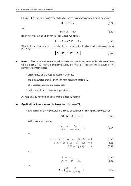
3.4 Generalized first-order kinetics* 50
Having B(), we can transform back into the original concentration basis by using
B = P −1 · A (3.69)
and
B 0 = P −1 · A 0 (3.70)
InsertingintooursolutionforB (Eq. 3.68), we obtain
P −1 · A = Λ P −1 · A 0 (3.71)
The final step is now a multiplication from the left with P which yields the solution for
Eq. 3.58
A = P · Λ P −1 · A 0 (3.72)
I Note: This may look complicated to someone who is not used to it. However, once
we have set up K, which is straightforward, everything is done by the computer: The
computer computes the
• eigenvalues of the rate constant matrix K,
• the eigenvector matrix P oftherateconstantmatrixK,
• all necessary inverse matrices, etc.,
• and does all the matrix multiplications.
All you usually have to do is to program the K matrix.
I
Application to our example (solution “by hand”):
• Evaluation of the eigenvalue matrix Λ by solution of the eigenvalue equation
det (K − Λ · I) =0 (3.73)
with I as unity matrix:
y
¯ − 1 − + 2
+ 1 − 2 − ¯ =0 (3.74)
(− 1 − ) · (− 2 − ) − ( 1 · 2 )=0 (3.75)
1 2 + 1 + 2 + 2 − 1 2 =0 (3.76)
( +( 1 + 2 )) = 0 (3.77)
y
1 =0 (3.78)
2 = − ( 1 + 2 ) (3.79)
y
Λ =
µ
0 0
0 − ( 1 + 2 )
(3.80)