IBR and Association rules

Overview
Prognostic Models and Data Mining
in Medicine, part II
Instance-based reasoning
1. Introduction
2. Case-based reasoning
3. Example: content-based image retrieval
4. k-NN classification
5. Case study: ICU prognosis
6. Summary
Includes material from:
- Tan, Steinbach, Kumar: Introduction to Data Mining
Prognostic Models and Data Mining, part II Instance-Based Reasoning 1
Prognostic Models and Data Mining, part II Instance-Based Reasoning 2
Instance-Based Reasoning
1. Introduction
Set of Stored Cases
Atr1 ……... AtrN Class
A
B
B
C
A
C
B
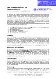
• Store the training records
• Select and use similar
training records to predict
the class label of unseen
cases
• No Model !
Unseen Case
Atr1 ……... AtrN
Prognostic Models and Data Mining, part II Instance-Based Reasoning 3
Prognostic Models and Data Mining, part II Instance-Based Reasoning 4
The Basic Idea ...
If it walks like a duck, quacks like a duck, then it’s
probably a duck.
Training
Records
Determine
similarity
Choose the most
similar records
Test
Record
The Flavors ...
• Case-based reasoning (CBR)
– alternative to reasoning with explicit
knowledge (e.g. IF-THEN rules)
– used in decision support systems
• k-Nearest Neighbours (k-NN) classification
– “lazy” machine learning method
– few assumptions, adapts to problem domain
Prognostic Models and Data Mining, part II Instance-Based Reasoning 5
Prognostic Models and Data Mining, part II Instance-Based Reasoning 6

The CBR paradigm
• Utilize specific knowledge of previously solved
problems to solve new problems.
2. Case-Based Reasoning (CBR)
• No need to formulate general rules about the
problem domain.
• Use intra-domain analogical reasoning
Prognostic Models and Data Mining, part II Instance-Based Reasoning 7
Prognostic Models and Data Mining, part II Instance-Based Reasoning 8
The CBR Cycle
Retrieve Step
Retained experience
New Problem
Case Library
RETRIEVE
Retrieved cases
REUSE
our
focus
• Find cases that are most similar to the current problem.
• Requires notion of similarity (“nearness”)
General properties:
1. s(x,x') ≥ 0 for all x and x'. (positiveness)
2. s(x,x') = 1 only if x = x'.
3. s(x,x') = s(x',x) for all x and x'. (symmetry)
RETAIN
Retrieved Solutions
• Common approach is to construct a distance metric d
for the feature space, and use s(x,x') = 1- d(x,x')/ d max ,
where d max is an upper limit on the distance.
Revised solution
REVISE
Prognostic Models and Data Mining, part II Instance-Based Reasoning 9
Prognostic Models and Data Mining, part II Instance-Based Reasoning 10
Distance Metrics (1)
Distance Metrics (2)
Triangle
inequality
Equal distance
“contour”s
Formally, for all objects x,x',x'' we should have that
– d(x,x') ≥ 0
(positiveness)
– d(x,x') = 0 iff x=x'
– d(x,x') = d(x',x) (symmetry)
– d(x,x'') ≤ d(x,x')+ d(x',x'') (triangle equality)
The best-known metric that satisfies these properties is
the Euclidean distance for objects in R m :
Symmetric nature of
distance functions
d(
x,
x' ) =
m
∑
i=
1
( x i
− x i
')
2
Prognostic Models and Data Mining, part II Instance-Based Reasoning 11
Prognostic Models and Data Mining, part II Instance-Based Reasoning 12

Minkowski Distance
Minkowski Distance
The Minkowski distance (also called power metric) is a
generalization of the Euclidean distance:
1
r
r
m
⎛ ⎞
d(
x,
x' ) = ⎜∑|
x i
− x i
'| ⎟
⎝ i=
1 ⎠
• r = 1. City block (Manhattan, taxicab, L 1
norm) distance.
– Called Hamming distance for binary vectors
• r = 2. Euclidean distance
• r →∞. “supremum” (L max
norm, L ∞
norm) distance.
– This is the maximum difference between any component of the
object.
point x y
p1 0 2
p2 2 0
p3 3 1
p4 5 1
L1 p1 p2 p3 p4
p1 0 4 4 6
p2 4 0 2 4
p3 4 2 0 2
p4 6 4 2 0
L2 p1 p2 p3 p4
p1 0 2.828 3.162 5.099
p2 2.828 0 1.414 3.162
p3 3.162 1.414 0 2
p4 5.099 3.162 2 0
L∞ p1 p2 p3 p4
p1 0 2 3 5
p2 2 0 1 3
p3 3 1 0 2
p4 5 3 2 0
Distance Matrix
Prognostic Models and Data Mining, part II Instance-Based Reasoning 13
Prognostic Models and Data Mining, part II Instance-Based Reasoning 14
Non-numeric attributes
• For non-numeric attributes, a dedicated distance measure
is required
• A simple solution for categorical attributes is to take
d(x i ,x i ')=0 if x i =x i ', and d(x i ,x i ')=1 otherwise
(Manhattan distance)
• More sophisticated solutions are possible when there
exists a (partial or complete) order on the categories
Scaling
• Weighed Minkowski distance
m
⎛
d(
x,
x' ) = ⎜∑
wi
| xi
− x
⎝ i=
1
1
r
r ⎞
i
'| ⎟
⎠
• Use w i =0 for attribute selection
• Problem: there exists no general method for assessing
the weights w i
Prognostic Models and Data Mining, part II Instance-Based Reasoning 15
Prognostic Models and Data Mining, part II Instance-Based Reasoning 16
Case-based reasoning in medicine
CBR is a popular methodology for building decision support
systems in the health sciences.
• Case histories are essential in the training of healthcare
professionals.
• The medical literature is filled with anecdotal accounts of
the treatments of individual patients.
• Many diseases are not well enough understood for formal
models or general guidelines.
• Reasoning from examples is natural for healthcare
professionals.
Advantages of CBR
• Intuitive problem-solving method.
• No need to formulate domain knowledge.
• Supports interactive way of finding solutions.
Disadvantages of CBR
• Can lead to copying mistakes from the past.
• Cases do not include knowledge of the domain, and this
handicaps explanation facilities.
Prognostic Models and Data Mining, part II Instance-Based Reasoning 17
Prognostic Models and Data Mining, part II Instance-Based Reasoning 18

Content-based image retrieval
• Digital images for diagnostics and therapy are produced
in ever-increasing quantities in medicine
3. Example: Content-based
image retrieval
• Access to relevant medical images can improve clinical
decisions
• Most convenient solution (for user) is content-based
retrieval of relevent images
• Content = colors, shapes, textures, or any other
information that can be derived from the image
• Sometimes also called visual query-by-example
Prognostic Models and Data Mining, part II Instance-Based Reasoning 19
Prognostic Models and Data Mining, part II Instance-Based Reasoning 20
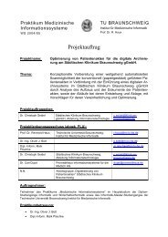
The ASSERT system (1)
The ASSERT system (2)
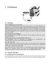
• Computer-aided diagnosis with computed tomographic
(CT) images of the chest (heart and lungs).
• When presented with a new image, the system retrieves
similar images with known diagnoses from the database.
• Preliminary validation: percentage of correct diagnoses
increased from 29% to 62% with computer assistance
(inexperienced doctors)
?
Emphysema
Emphysema
A.M. Aisen et al., Radiology 2003;228:265-70.
Macro nodules
Micro nodules
Prognostic Models and Data Mining, part II Instance-Based Reasoning 21
Prognostic Models and Data Mining, part II Instance-Based Reasoning 22
The ASSERT system (3)
4. k-Nearest k
Neighbor (k-NN) Classification
Prognostic Models and Data Mining, part II Instance-Based Reasoning 23
Prognostic Models and Data Mining, part II Instance-Based Reasoning 24

Nearest-Neighbor Classification
Nearest-Neighbor Classifiers
• Classification method from ML that resembles casebased
reasoning.
• Key idea: to classify an object x, locate the nearest
object(s) in the training set, and look at its/their class(es)
• Avoids constructing a model, instead classifies directly
from the data (“lazy learning”)
new object
• Requires three things
– The set of stored objects
– Distance Metric to compute
distance between objects
– The value of k, the number of
nearest neighbors to retrieve
• To classify a new object:
– Compute distance to other
training objects
– Identify k nearest neighbors
– Use class labels of nearest
neighbors to determine the
class label of new object
(e.g., by taking majority vote)
Prognostic Models and Data Mining, part II Instance-Based Reasoning 25
Prognostic Models and Data Mining, part II Instance-Based Reasoning 26
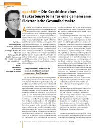
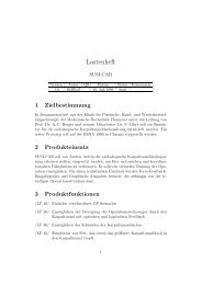
Definition of Nearest Neighbor
Example
X X X
(a) 1-nearest neighbor (b) 2-nearest neighbor (c) 3-nearest neighbor
k-nearest neighbors of a object x are data points that
have the k smallest distance to x
1
2
3
4
5
6
7
8
9
0
0
-2
0
2
-2
-5
1
-2
x 2
0
-3
-2
5
3
2
0
1
0
x 3
T
F
F
T
T
T
F
T
F
y
−
−
−
+
+
+
+
?
?
2
18
19
17
5
10
1-NN: −
3-NN: +
x 1
38
Prognostic Models and Data Mining, part II Instance-Based Reasoning 27
Prognostic Models and Data Mining, part II Instance-Based Reasoning 28
Example
1 nearest-neighbor
1
2
3
4
5
6
7
8
9
x 1
9
0
0
-2
0
2
-2
-5
1
-2
x 2
0
-3
-2
5
3
2
0
1
0
x 3
T
F
F
T
T
T
F
T
F
y
−
−
−
+
+
+
+
?
?
5
13
4
30
14
5
1-NN: −
3-NN: −
Voronoi Diagram
Prognostic Models and Data Mining, part II Instance-Based Reasoning 29
Prognostic Models and Data Mining, part II Instance-Based Reasoning 30

How many Neighbors? (1)
• Choosing the value of k:
– If k is too small, sensitive to noise points
– If k is too large, neighborhood may include points from
other classes
How many Neighbors? (2)
• A possible solution is to determine the optimal value of k
using the data
• That is, we try different values of k, and choose the one
that performs best ...
• ... on a test set, or with cross-validation (Why?)
• This is basically the same solution as choosing the
optimal size of a decision tree by post-pruning
• If we also want to evaluate the final k-NN classifier,
we have to use another, separate test set
• ... or an outer cross-validation loop
Prognostic Models and Data Mining, part II Instance-Based Reasoning 31
Prognostic Models and Data Mining, part II Instance-Based Reasoning 32
Classification rules
Determine the class from nearest neighbor list
• Take the majority vote of class labels among
the k-nearest neighbors
• Weigh the vote according to distance:
k
∑ w
j=
j
y
1 j
1
P(
y | xq
) = where w
k
j
=
2
w
d( x , x )
∑
j=
1
j
q
j
Scaling issues
• Attributes may have to be scaled to prevent distance
measures from being dominated by one of the attributes
• Example:
– height of a person may vary from 1.5m to 1.8m
– weight of a person may vary from 90lb to 300lb
– income of a person may vary from $10K to $1M
Note: now it makes sens to use all training objects,
instead of just k (Shepard’s method).
Prognostic Models and Data Mining, part II Instance-Based Reasoning 33
Prognostic Models and Data Mining, part II Instance-Based Reasoning 34
Curse of Dimensionality
• When dimensionality
increases, data becomes
increasingly sparse in the
space that it occupies
• Definitions of density and
distance between points,
which is critical for k-NN,
become less meaningful
Lazy learning
• k-NN classifiers are lazy learners
– No models are built, unlike eager learners such as
decision tree induction and rule-based systems.
– Classifying new objects is relatively expensive.
• k-NN is easily misled in
high-dimensional spaces
• Randomly generate 500 points
• Compute difference between max and min
distance between any pair of points
Prognostic Models and Data Mining, part II Instance-Based Reasoning 35
Prognostic Models and Data Mining, part II Instance-Based Reasoning 36

Advantages of k-NN
• No assumptions on model form (no inductive bias):
very flexible ML method.
• Training is very fast.
• No loss of information.
Disadvantages of k-NN
• Requires more data than eager learners to obtain the
same perforance.
• Classifying new objects can be slow.
• Curse of dimensionality: does not work in
high-dimensional spaces.
5. Case study: ICU prognosis
Joint work with Clarence Tan and Linda Peelen.
Prognostic Models and Data Mining, part II Instance-Based Reasoning 37
Prognostic Models and Data Mining, part II Instance-Based Reasoning 38
Prognosis in intensive care
Scoring
LR model
Patient data Score Probability
sheet
• Case–mix correction of outcomes (mortality)
for benchmarking and institutional comparison.
• Prediction: probability of hospital death.
• Based on APACHE II score.
Scoring
k-NN
Patient data Score Probability
sheet
Prognostic Models and Data Mining, part II Instance-Based Reasoning 39 Prognostic Models and Data Mining, part II Instance-Based Reasoning 40
Why k-NN?
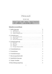
k-NN regression
• Logistic regression assumes fixed relationship between
case-mix (score) and outcome – may not hold.
• Logistic regression model becomes outdated after time
(sensitive to drift)
+
+
+
But ...
• k-NN requires large dataset
a2
-
X
-
-
1-NN regression
estimate for X: 1
• k-NN works only in low-dimensional domains
-
+
+
-
5-NN regression
estimate for X: 0.4
a1
Prognostic Models and Data Mining, part II Instance-Based Reasoning 41
Prognostic Models and Data Mining, part II Instance-Based Reasoning 42

Kernel regression
How many neighbors?
Similar to weighted k-NN, but uses a predefined kernel
function to transform (normalized) distances into weights.
• Problem: how many neighbors should we have in the
neighborhood?
• Solution: Depends on problem, learn from the data!
Uniform
Tri-cube
Epanechnikov
Prognostic Models and Data Mining, part II Instance-Based Reasoning 43
Prognostic Models and Data Mining, part II Instance-Based Reasoning 44
Choosing the neighborhood size
Model validation
R-squared
Validating a prognostic model means establishing that the
model works satisfactorily for patients other than those from
whose data it was derived.
Like for any other scientific hypothesis, the validity of a
model is established by gathering incremental evidence
across diverse settings.
Neighborhood size
Prognostic Models and Data Mining, part II Instance-Based Reasoning 45
Prognostic Models and Data Mining, part II Instance-Based Reasoning 46
Types of validity
Prospective validation
• Internal validity
The model is valid for patients from the same population
and in the same setting.
• Prospective validity
The model is valid for future patients from the same
population and in the same setting.
• External validity
The model is valid for patients from another population or
another setting.
Does the k-NN prediction method generalize well to
prospective data?
Training
set
Kernel parameter settings
Instance
base
IBR
Results
Validation
set
Queries
Prognostic Models and Data Mining, part II Instance-Based Reasoning 47
Prognostic Models and Data Mining, part II Instance-Based Reasoning 48

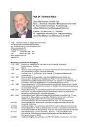
Prospective validation: results
Incremental prospective validation
AUC
Internal
validation
Prospective
validation
LR model
Does the method generalize well while adding data?
– ICU admissions with known outcomes become
examples for new instances
APACHE
0.792
0.784
0.804
SAPS
0.860
0.867
0.877
Training
set
Kernel parameter settings
Add when
outcome is known
Instance
base
IBR
Results
Validation
set
Queries
Prognostic Models and Data Mining, part II Instance-Based Reasoning 49
Prognostic Models and Data Mining, part II Instance-Based Reasoning 50
Incremental prospective validation
AUC
Plain
prospective
validation
Incremental
prospective
validation
LR model
APACHE
0.784
0.809
0.804
SAPS
0.867
0.867
0.877
6. Summary
Prognostic Models and Data Mining, part II Instance-Based Reasoning 51
Prognostic Models and Data Mining, part II Instance-Based Reasoning 52
Summary: CBR and k-NN
• Case-based reasoning is a methodology to build advice
systems. It utilizes experience of previously solved
problems to solve new problems.
• k-NN is a supervised machine learning method, that
avoids to construct a model and classifies new objects
directly from the training data.
• Both methods are very flexible because they do not try to
exploit general rules – but this also means that they
provide no new insights.
• The notion of similarity/distance is central to both
approaches.
Prognostic Models and Data Mining, part II Instance-Based Reasoning 53

Overview
Prognostic Models and Data Mining
in Medicine, part II
Association Rule Discovery
1. Introduction
2. Frequent Itemset Generation
3. Rule Generation
4. Interpretaion and Evaluation
5. Application: Hospital Infection Control
6. Summary
Includes material from:
- Tan, Steinbach, Kumar: Introduction to Data Mining
- Witten & Frank: Data Mining. Practical Machine Learning Tools and Techniques
Prognostic Models and Data Mining, part II Association Rule Discovery 1
Prognostic Models and Data Mining, part II Association Rule Discovery 2
Association Rule Discovery: Definition
• Given a set of records each of which contain some
number of items (“transaction”) from a given collection:
• Produce dependency rules which will predict occurrence
of an item based on occurrences of other items.
1. Introduction
TID Items
1 Bread, Coke, Milk
2 Beer, Bread
3 Beer, Coke, Diaper, Milk
4 Beer, Bread, Diaper, Milk
5 Coke, Diaper, Milk
Rules Discovered:
{Milk} {Milk} → {Coke}
{Diaper, Milk} Milk} → {Beer}
Implication means co-occurrence,
not causality!
Prognostic Models and Data Mining, part II Association Rule Discovery 3
Prognostic Models and Data Mining, part II Association Rule Discovery 4
Associational learning
Definition: Frequent Itemset
• Can be applied if no class is specified and any
kind of structure is considered “interesting”
• Difference to classification learning:
– Can predict any attribute’s value, not just the class,
and more than one attribute’s value at a time
– Hence: far more association rules than classification
rules
– Thus: constraints are necessary
– Minimum coverage and minimum accuracy
• Itemset
– A collection of one or more items
Example: {Milk, Bread, Diaper}
– k-itemset
An itemset that contains k items
• Support count (σ)
– Frequency of occurrence of an itemset
– E.g. σ({Milk, Bread,Diaper}) = 2
• Support
– Fraction of transactions that contain an
itemset
– E.g. s({Milk, Bread, Diaper}) = 2/5
• Frequent Itemset
– An itemset whose support is greater
than or equal to a minsup threshold
TID
Items
1 Bread, Milk
2 Bread, Diaper, Beer, Eggs
3 Milk, Diaper, Beer, Coke
4 Bread, Milk, Diaper, Beer
5 Bread, Milk, Diaper, Coke
Prognostic Models and Data Mining, part II Association Rule Discovery 5
Prognostic Models and Data Mining, part II Association Rule Discovery 6

Definition: Association Rule
• Association Rule
– An implication expression of the form
X → Y, where X and Y are itemsets
– Example:
{Milk, Diaper} → {Beer}
• Rule Evaluation Metrics
– Support (s)
Fraction of transactions that contain
both X and Y
– Confidence (c)
Measures how often items in Y
appear in transactions that
contain X
TID Items
1 Bread, Milk
2 Bread, Diaper, Beer, Eggs
3 Milk, Diaper, Beer, Coke
4 Bread, Milk, Diaper, Beer
5 Bread, Milk, Diaper, Coke
Example:
{ Milk, Diaper} ⇒ Beer
(Milk,Diaper,Beer) 2
s = σ
= = 0.4
| T | 5
σ (Milk,Diaper,Beer) 2
c =
= = 0.67
σ (Milk,Diaper) 3
Prognostic Models and Data Mining, part II Association Rule Discovery 7
Association Rule Mining Task
• Given a set of transactions T, the goal of
association rule mining is to find all rules having
– support ≥ minsup threshold
– confidence ≥ minconf threshold
• Brute-force approach:
– List all possible association rules
– Compute the support and confidence for each rule
– Prune rules that fail the minsup and minconf
thresholds
→ Computationally prohibitive!
Prognostic Models and Data Mining, part II Association Rule Discovery 8
Mining Association Rules
TID
Items
1 Bread, Milk
2 Bread, Diaper, Beer, Eggs
3 Milk, Diaper, Beer, Coke
4 Bread, Milk, Diaper, Beer
5 Bread, Milk, Diaper, Coke
Observations:
Example of Rules:
{Milk,Diaper} → {Beer} (s=0.4, c=0.67)
{Milk,Beer} → {Diaper} (s=0.4, c=1.0)
{Diaper,Beer} → {Milk} (s=0.4, c=0.67)
{Beer} → {Milk,Diaper} (s=0.4, c=0.67)
{Diaper} → {Milk,Beer} (s=0.4, c=0.5)
{Milk} → {Diaper,Beer} (s=0.4, c=0.5)
• All the above rules are binary partitions of the same itemset:
{Milk, Diaper, Beer}
• Rules originating from the same itemset have identical support but
can have different confidence
• Thus, we may decouple the support and confidence requirements
Prognostic Models and Data Mining, part II Association Rule Discovery 9
Mining Association Rules
• Two-step approach:
1. Frequent Itemset Generation
– Generate all itemsets whose support ≥ minsup
2. Rule Generation
– Generate high confidence rules from each frequent itemset,
where each rule is a binary partitioning of a frequent itemset
• Frequent itemset generation is still
computationally expensive
Prognostic Models and Data Mining, part II Association Rule Discovery 10
Frequent Itemset Generation
null
A B C D E
2. Frequent Itemset Generation
AB AC AD AE BC BD BE CD CE DE
ABC ABD ABE ACD ACE ADE BCD BCE BDE CDE
ABCD ABCE ABDE ACDE BCDE
ABCDE
Given d items, there
are 2 d possible
candidate itemsets
Prognostic Models and Data Mining, part II Association Rule Discovery 11
Prognostic Models and Data Mining, part II Association Rule Discovery 12

Reducing Number of Candidates
Illustrating Apriori Principle
• Apriori principle:
– If an itemset is frequent, then all of its subsets must also
be frequent
• Apriori principle holds due to the following property
of the support measure:
∀X
, Y : ( X ⊆ Y ) ⇒ s(
X ) ≥ s(
Y )
Found to be
Infrequent
– Support of an itemset never exceeds the support of its
subsets
– This is known as the anti-monotone property of support
Prognostic Models and Data Mining, part II Association Rule Discovery 13
Pruned
supersets
Prognostic Models and Data Mining, part II Association Rule Discovery 14
Illustrating Apriori Principle
Apriori Algorithm
Item Count
Bread 4
Coke 2
Milk 4
Beer 3
Diaper 4
Eggs 1
Minimum Support = 3
If every subset is considered,
6 C 1 + 6 C 2 + 6 C 3 = 41
With support-based pruning,
6 + 6 + 1 = 13
Items (1-itemsets)
Itemset
Count
{Bread,Milk} 3
{Bread,Beer} 2
{Bread,Diaper} 3
{Milk,Beer} 2
{Milk,Diaper} 3
{Beer,Diaper} 3
Pairs (2-itemsets)
(No need to generate
candidates involving Coke
or Eggs)
Triplets (3-itemsets)
Item set
Count
{B read,M ilk,D iaper} 3
• Method:
– Let k=1
– Generate frequent itemsets of length 1
– Repeat until no new frequent itemsets are identified
Generate length (k+1) candidate itemsets from length k
frequent itemsets
Prune candidate itemsets containing subsets of length k that
are infrequent
Count the support of each candidate by scanning the DB
Eliminate candidates that are infrequent, leaving only those
that are frequent
Prognostic Models and Data Mining, part II Association Rule Discovery 15
Prognostic Models and Data Mining, part II Association Rule Discovery 16
Example
Maximal Frequent Itemset
TID
1
2
3
4
5
6
7
8
Items
A,B,C,D
A,C,D,F
C,D,E,G,A
A,D,F,B
B,C,G
D,F,G
A,B,G
C,D,F,G
Itemsets with minsup=33%:
• A:5, B:4, C:5, D:6, E:1, F:4, G:5
• AB:3, AC:3, AD:3, AF:2, AG:2,
BC:2, BD:2, BF:1, BG:2, CD:4,
CF:2, CG:3, DF:4, DG:3, FG:2
• ABC:1, ABD:2, ACD:3, CDG:2,
CDF:2, DFG:2
• Done
An itemset is maximal frequent if none of its immediate
supersets is frequent
Maximal
Itemsets
Infrequent
Itemsets
Border
Prognostic Models and Data Mining, part II Association Rule Discovery 17
Prognostic Models and Data Mining, part II Association Rule Discovery 18

Closed Itemset
Maximal vs Closed Itemsets
An itemset is closed if none of its immediate supersets has
the same support as the itemset
TID Items
1 {A,B}
2 {B,C,D}
3 {A,B,C,D}
4 {A,B,D}
5 {A,B,C,D}
Itemset Support
{A} 4
{B} 5
{C} 3
{D} 4
{A,B} 4
{A,C} 2
{A,D} 3
{B,C} 3
{B,D} 4
{C,D} 3
Itemset Support
{A,B,C} 2
{A,B,D} 3
{A,C,D} 2
{B,C,D} 3
{A,B,C,D} 2
TID Items
1 ABC
2 ABCD
3 BCE
4 ACDE
5 DE
Transaction Ids
null
124 123 1234 245 345
A B C D E
12
AB
124
AC
24
AD
4 123 2 3 24 34 45
AE BC BD BE CD CE DE
12 2 24 4 4 2 3 4
ABC ABD ABE ACD ACE ADE BCD BCE BDE CDE
2 4
ABCD ABCE ABDE ACDE BCDE
Not supported by
any transactions
ABCDE
Prognostic Models and Data Mining, part II Association Rule Discovery 19
Prognostic Models and Data Mining, part II Association Rule Discovery 20
Maximal vs Closed Frequent Itemsets
Maximal vs Closed Itemsets
Minimum support = 2
null
Closed but
not maximal
124 123 1234 245 345
A B C D E
Closed and
maximal
12
AB
124
AC
24
AD
4 123 2 3 24 34 45
AE BC BD BE CD CE DE
12 2 24 4 4 2 3 4
ABC ABD ABE ACD ACE ADE BCD BCE BDE CDE
2 4
ABCD ABCE ABDE ACDE BCDE
# Closed = 9
# Maximal = 4
ABCDE
Prognostic Models and Data Mining, part II Association Rule Discovery 21
Prognostic Models and Data Mining, part II Association Rule Discovery 22
Rule Generation
3. Rule Generation
• Given a frequent itemset L, find all non-empty
subsets f ⊂ L such that f → L – f satisfies the
minimum confidence requirement
– If {A,B,C,D} is a frequent itemset, candidate rules:
ABC →D, ABD →C, ACD →B, BCD →A,
A →BCD, B →ACD, C →ABD, D →ABC
AB →CD, AC → BD, AD → BC, BC →AD,
BD →AC, CD →AB,
• If |L| = k, then there are 2 k – 2 candidate
association rules (ignoring L → ∅and ∅ →L)
Prognostic Models and Data Mining, part II Association Rule Discovery 23
Prognostic Models and Data Mining, part II Association Rule Discovery 24

Rule Generation
• How to efficiently generate rules from frequent
itemsets?
– In general, confidence does not have an antimonotone
property
c(ABC →D) can be larger or smaller than c(AB →D)
Rule Generation for Apriori Algorithm
Lattice of rules
Low
Confidence
Rule
– But confidence of rules generated from the same
itemset has an anti-monotone property
– e.g., L = {A,B,C,D}:
c(ABC → D) ≥ c(AB → CD) ≥ c(A → BCD)
Confidence is anti-monotone w.r.t. number of items on the
RHS of the rule
Pruned
Rules
Prognostic Models and Data Mining, part II Association Rule Discovery 25
Prognostic Models and Data Mining, part II Association Rule Discovery 26
Rule Generation for Apriori Algorithm
• Candidate rule is generated by merging two rules
that share the same prefix
in the rule consequent
CD=>AB
BD=>AC
• join(CD=>AB,BD=>AC)
would produce the candidate
rule D => ABC
4. Interpretation & Evaluation
• Prune rule D=>ABC if its
subset AD=>BC does not have
high confidence
D=>ABC
Prognostic Models and Data Mining, part II Association Rule Discovery 27
Prognostic Models and Data Mining, part II Association Rule Discovery 28
Interpreting association rules
• Interpretation is not obvious:
If windy = false and play = no then outlook = sunny
and humidity = high
is not the same as
If windy = false and play = no then outlook = sunny
If windy = false and play = no then humidity = high
• It means that the following also holds:
Evaluating Association Rules
• Association rule algorithms tend to produce too
many rules
– many of them are uninteresting or redundant
– Redundant if {A,B,C} → {D} and {A,B} → {D}
have same support & confidence
• Interestingness measures can be used to
prune/rank the derived patterns
If humidity = high and windy = false and play = no
then outlook = sunny
Prognostic Models and Data Mining, part II Association Rule Discovery 29
Prognostic Models and Data Mining, part II Association Rule Discovery 30

Computing Interestingness Measure
Drawback of Confidence
• Given a rule X → Y, information needed to compute rule
interestingness can be obtained from a contingency table
Contingency table for X → Y
Y Y
X f 11 f 10 f 1+
X f 01 f 00 f o+
f +1 f +0 |T|
f 11 : support of X and Y
f 10 : support of X and Y
f 01 : support of X and Y
f 00 : support of X and Y
Used to define various measures
support, confidence, lift, Gini,
J-measure, etc.
Coffee Coffee
Tea 15 5 20
Tea 75 5 80
90 10 100
Association Rule: Tea → Coffee
Confidence= P(Coffee|Tea) = 0.75
but P(Coffee) = 0.9
⇒ Although confidence is high, rule is misleading
⇒ P(Coffee|Tea) = 0.9375
Prognostic Models and Data Mining, part II Association Rule Discovery 31
Prognostic Models and Data Mining, part II Association Rule Discovery 32
Other measures of association
Example: Lift
P(
Y | X )
Lift =
(sometimes called “interest”)
P(
Y )
PS = P(
X , Y ) − P(
X ) P(
Y )
P(
X , Y ) − P(
X ) P(
Y )
φ − coefficient =
P(
X )[1 − P(
X )] P(
Y )[1 − P(
Y )]
Coffee Coffee
Tea 15 5 20
Tea 75 5 80
90 10 100
Association Rule: Tea → Coffee
Confidence= P(Coffee|Tea) = 0.75
but P(Coffee) = 0.9
⇒ Lift = 0.75/0.9= 0.8333 (< 1, therefore is negatively associated)
Prognostic Models and Data Mining, part II Association Rule Discovery 33
Prognostic Models and Data Mining, part II Association Rule Discovery 34
Biosurveillance systems
5. Application: Biosurveillance systems
• Biosurveillance systems are computer programs for early
detection of infectious outbreaks.
• Hospitals environments (and especially ICUs) are liable
to outbreaks of infections, but outbreaks can also occur
elsewhere.
• Traditionally, biosurveillance systems assume a
predefined event whose incidence is to be monitored.
Prognostic Models and Data Mining, part II Association Rule Discovery 35
Prognostic Models and Data Mining, part II Association Rule Discovery 36

Traditional Approaches (1)
• Various methods have
been developed for
monitoring event data:
– Time series analysis
– Regression techniques
– Statistical Quality Control
methods
Number of ED Visits per Day
• Problem: We need to know in advance which events should
be monitored.
• We cannot focus on other characteristics (e.g. spatial or
demographic) of an epidemic.
Number of ED Visits
50
40
30
20
10
0
1
10
19
28
37
46
55
64
73
82
91
100
Day Number
Traditional Approaches (2)
We need to build a univariate detector to monitor each
interesting combination of attributes:
Diarrhea cases
among children
Respiratory syndrome
Number of cases involving
cases You’ll among need females hundreds of teenage univariate girls detectors!
living in the
We would like to identify the groups western with part of the strangest city
Viral syndrome cases
involving senior behavior citizens in recent events.
from eastern part of city Botulinic syndrome cases
Number of children from
downtown hospital
Number of cases involving
people working in southern
part of the city
And so on…
Prognostic Models and Data Mining, part II Association Rule Discovery 37
Prognostic Models and Data Mining, part II Association Rule Discovery 38
The approach from Brossette et al. (1)
1. For each time window (e.g. one month), discover all
high-support association rules.
2. The confidence of each rule discovered in the current
slice is compared with its confidence in previous slices.
3. If the confidence has changed significantly, this is
reported to the user.
The approach from Brossette et al. (2)
Advantages:
• Not limited to a single event.
• Can take other characteristics of epidemic (e.g. location)
into account.
Disadvantages:
• The method is statistically poorer than traditional
approaches. Some “significant” changes in rule
confidence will occur due to chance.
• The patterns identified by the analysis are only
potentially interesting; further examination will be
needed.
Prognostic Models and Data Mining, part II Association Rule Discovery 39
Prognostic Models and Data Mining, part II Association Rule Discovery 40
Summary
• Association rules describe co-occurrence of items within
transaction data.
6. Summary
• Association rules are discovered in two steps:
1. Frequent Itemset Generation (focus on support)
2. Rule Generation (focus on confidence)
• Often, additional measures of “interestingness” are
needed to filter the discovered rules. This is non-trivial.
Prognostic Models and Data Mining, part II Association Rule Discovery 41
Prognostic Models and Data Mining, part II Association Rule Discovery 42