LIMITATIONS OF GAUGE INVARIANCE
LIMITATIONS OF GAUGE INVARIANCE
LIMITATIONS OF GAUGE INVARIANCE

You also want an ePaper? Increase the reach of your titles
YUMPU automatically turns print PDFs into web optimized ePapers that Google loves.
<strong>LIMITATIONS</strong> <strong>OF</strong> <strong>GAUGE</strong> <strong>INVARIANCE</strong><br />
and<br />
CONSEQUENCES FOR LASER-INDUCED PROCESSES<br />
This lecture is based on a talk given at the<br />
Joint Theoretical Colloquium of ETH Zurich and University of Zürich on 17 May 2010.<br />
1
PREAMBLE<br />
• Physical processes involving electromagnetic interactions depend<br />
entirely on the electric and magnetic fields that are present.<br />
• These fields can be represented as derivatives of scalar and vector<br />
potential functions that are often mathematically convenient, but are<br />
actually only auxiliary quantities. (Each such set is called a gauge.)<br />
• The potential functions are not unique. There are many sets of these<br />
functions corresponding to the same fields and thus to the same<br />
physical processes. (They are connected by gauge transformations.)<br />
• The choice of which of the possible sets of potentials to use for a given<br />
problem is a matter of mathematical or conceptual convenience.<br />
• Exactly the same considerations about the choice of gauge apply to<br />
both classical and quantum phenomena.<br />
Not one of the above statements is entirely correct.<br />
2
Furthermore…<br />
There is another set of statements that is accepted almost universally in<br />
the Atomic, Molecular, and Optical (AMO) physics community, and to<br />
some extent outside that community:<br />
• A gauge transformation is a unitary transformation.<br />
• Quantum transition amplitudes are manifestly gauge invariant.<br />
Less universal, but also widespread:<br />
• The most basic approach is to formulate all problems using a scalar<br />
potential. (Within the dipole approximation, this is called the length<br />
gauge.) If a different gauge is desired, this should be obtained through a<br />
gauge transformation from the length gauge.<br />
All of the bulleted statements above are false.<br />
3
OUTLINE<br />
• Review the rules for gauges and gauge transformations.<br />
• Examine an elementary one-dimensional classical example to illustrate some of the<br />
problems to be explored.<br />
• Show how conservation conditions can be changed by gauge transformations.<br />
• Examine the essential differences between Newtonian mechanics and other<br />
formulations.<br />
• Examples from strong-field physics. (Many gauge transformation difficulties are<br />
exacerbated by strong fields.)<br />
• Exhibit an essential difference between the properties of classical and quantum<br />
gauge transformations.<br />
• Show how the above demonstration solves some essential long-standing dilemmas in<br />
the foundations of strong-field physics.<br />
• The above considerations infer the existence of a physical gauge. (This is still<br />
controversial and not essential.)<br />
• Revisit the statements from the Preamble.<br />
4
ELECTROMAGNETIC POTENTIALS<br />
Electric fields E and magnetic fields B can be written in terms of scalar<br />
potentials vector potentials A through the connections (Gaussian<br />
units)<br />
When substituted into Maxwell’s equations, and with the Lorentz<br />
condition<br />
enforced in order to decouple the and A equations, the result is the<br />
wave equations<br />
where is a charge density and J is a current density.<br />
5
FOOTNOTES ABOUT THE LORENTZ CONDITION<br />
One of the senior participants in the Joint Theoretical Physics Colloquium expressed a dislike for<br />
the Lorentz condition.<br />
I disagree, based on its necessity for decoupling the inhomogeneous wave equations for scalar<br />
and vector potentials. Arguments based on approximations that relieve the necessity for strict<br />
adherence to the Lorentz condition become questionable when fields are strong.<br />
There is a superficial discrepancy in the LG, where A = 0 and /t 0, but this is not essential<br />
because there is no wave equation for A from which to decouple. However, the fact that<br />
/t 0 IS important because the wave equation for then requires a source density ,<br />
whereas a plane wave does not require any sources. This just emphasizes the unphysical nature<br />
of the LG for description of PW phenomena.<br />
There is a separate issue with the Coulomb gauge. It is stated in many textbooks (including<br />
Jackson) that a defining condition for the Coulomb gauge is that A= 0.<br />
That condition, plus the constraint = 0 , leads to the Lorentz condition being satisfied.<br />
However, there is no covariant (completely relativistic) equivalent for this, whereas the Lorentz<br />
condition in its full form does have a covariant statement.<br />
6
<strong>GAUGE</strong> TRANSFORMATION<br />
If is any scalar function that satisfies the homogeneous wave equation<br />
then the gauge transformation<br />
leaves the electric and magnetic fields unchanged.<br />
LORENTZ FORCE<br />
A particle of charge q, subjected to an electric field E and a magnetic field B while<br />
moving with velocity v will experience a force F Lorentz :<br />
7
NEWTONIAN EQUATION <strong>OF</strong> MOTION<br />
The trajectory of motion of a particle of charge q and mass m subjected<br />
to an electromagnetic field is given by the solution of the Newtonian<br />
equation of motion<br />
The trajectory depends only on the force.<br />
The force depends only on the fields E and B.<br />
The fields are unchanged by a gauge transformation.<br />
Therefore the solution of the problem is gauge invariant.<br />
The analysis above has long been accepted as conclusive evidence for<br />
gauge invariance as a fundamental and unambiguous principle of<br />
electrodynamics.<br />
8
THERE ARE HINTS <strong>OF</strong> BASIC PROBLEMS<br />
For example:<br />
• The equations of quantum mechanics are all in terms of potentials and<br />
not fields. Many attempts have been made to write the Schrödinger<br />
equation directly in terms of E and B, but none have succeeded. All such<br />
attempts have yielded nonlocal formulations.<br />
• In textbooks on classical mechanics it is common to find<br />
demonstrations that alternative formulations (Hamiltonian, Lagrangian,<br />
…, expressed in terms of potentials) can be shown to infer Newton’s<br />
equations, but not the converse.<br />
• In strong-field physics, two gauges are in common use, and they can be<br />
shown to contradict each other in fundamental ways.<br />
9
An elementary example illustrates basic problems with gauge invariance<br />
A CHARGED PARTICLE IN A CONSTANT ELECTRIC FIELD<br />
ONE-DIMENSIONAL TREATMENT<br />
Classical electrostatics is a complete field in itself. It can be done<br />
exclusively with scalar potentials.<br />
Elementary example: a particle of mass m and charge q in a constant<br />
electric field E 0 . This can be done in one dimension x.<br />
Hamiltonian: H = p 2 /2m – qE 0 x<br />
Hamilton’s equations:<br />
x<br />
<br />
H<br />
p<br />
<br />
p<br />
m<br />
;<br />
p<br />
<br />
H<br />
x<br />
<br />
qE 0<br />
10
These equations can be combined to give:<br />
x<br />
qE ,<br />
m<br />
0<br />
This is Newton’s equation: (mass)(acceleration) = force<br />
The solution is elementary; it is quadratic in time.<br />
Now a simple gauge transformation will be applied.<br />
What has been done above corresponds to what is often called the<br />
length gauge, because the interaction term in the Hamiltonian has the<br />
form – E 0 x . The gauge transformation to be applied eliminates the<br />
scalar potential and introduces a one-dimensional version of a vector<br />
potential. This is called the velocity gauge.<br />
The gauge transformation has the generating function<br />
= - cE 0 x t<br />
11
<strong>GAUGE</strong> TRANSFORMATION<br />
1 <br />
xE0<br />
' 0<br />
c t<br />
<br />
A 0 A'<br />
A cE0t<br />
x<br />
2<br />
p<br />
1<br />
H qxE0 H ' p ' qE0t<br />
2m<br />
2m<br />
Transformed Hamilton’s equations are:<br />
x<br />
H'<br />
p ' qE t H'<br />
, ' 0<br />
p ' m x<br />
0<br />
p <br />
mx<br />
<br />
qE<br />
These equations can be combined to give: 0<br />
THE EQUATION <strong>OF</strong> MOTION IS AS BEFORE.<br />
<strong>GAUGE</strong> <strong>INVARIANCE</strong> IS SATISFIED!<br />
<br />
2<br />
12
<strong>GAUGE</strong> EQUIVALENT – BUT DIFFERENT<br />
The most obvious difference is in the conservation of energy.<br />
Written as H = kinetic energy + potential energy = T + V:<br />
H<br />
T<br />
H' T'<br />
V<br />
<br />
constan t<br />
t<br />
;<br />
V' 0<br />
Evaluated with respective solutions: T = T' as expected.<br />
This must be so because kinetic energy is measurable in the laboratory<br />
and must be preserved by a gauge transformation.<br />
HOWEVER: V V . THIS IS A FUNDAMENTAL DIFFERENCE.<br />
In the original gauge, potential energy is converted into kinetic energy.<br />
After the gauge transformation, kinetic energy grows as t 2 with no<br />
source for this unlimited energy.<br />
13
CONSERVATION PRINCIPLES<br />
If the Hamiltonian (or Lagrangian) is independent of a particular generalized<br />
coordinate, then the conjugate generalized momentum is conserved. This applies in as<br />
many generalized coordinates as exist in the problem.<br />
H<br />
p 0 p<br />
const.<br />
x<br />
In particular, if the Hamiltonian is independent of time, then energy is conserved, if H<br />
= H(t) explicitly, then energy is not conserved.<br />
Compare: H = p 2 /2m – qE 0 x<br />
with: H’ = (1/2m)(p’ + qE 0 t) 2<br />
In general, if a particular Hamiltonian is independent of some generalized coordinate<br />
x, the conjugate momentum p is conserved; if the generating function for a gauge<br />
transformation introduces a dependence on x, then p is not conserved.<br />
That is, introducing a gauge transformation<br />
makes it possible to alter conservation conditions.<br />
14
NEWTONIAN MECHANICS DIFFERS FROM OTHER FORMULATIONS<br />
It has just been seen that symmetries of the Hamiltonian (or Lagrangian)<br />
function provides information about conservation conditions.<br />
H or L are system functions containing information that is not present in<br />
Newtonian mechanics; these system functions depend on potentials.<br />
System functions cannot be written directly in terms of fields unless<br />
there is resort to nonlocal formalisms.<br />
Conclusion: Potentials contain more information than do the fields.<br />
15
PHYSICAL <strong>GAUGE</strong><br />
Electrostatics can be formulated self-consistently with scalar potentials<br />
alone. Any gauge transformation will preserve the particle trajectory,<br />
but will introduce some unphysical feature such as the failure of energy<br />
conservation. Implication: there exists a gauge that is entirely physical.<br />
For electrostatics, the physical gauge is the gauge with only a scalar<br />
potential and no vector potential.<br />
0, A = 0<br />
Static (and quasistatic) fields are called longitudinal fields.<br />
The electric field follows field lines from one plate of a parallel plate<br />
capacitor to the other. This can be viewed as the “propagation” of the<br />
electric field in a direction parallel to the polarization direction.<br />
Any gauge transformation from the physical gauge introduces some<br />
feature(s) that are nonphysical,<br />
even though gauge invariance holds true.<br />
16
CAUTIONS ABOUT THE “PHYSICAL <strong>GAUGE</strong>” CONCEPT<br />
The concept is: every gauge transformation induces some alteration in<br />
physical interpretation; therefore, there can be only one gauge that<br />
matches laboratory conditions in every respect.<br />
This concept has been criticized on the grounds of an insufficiently<br />
precise definition of the “physical gauge”.<br />
So far, the debate has engaged only a small number of qualified people.<br />
The long-term outcome is still in doubt.<br />
Interim advice: unless you relish tough debates, avoid this concept for<br />
now. (Personally, I think it is a very useful idea, and I believe the issue<br />
was actually settled long ago: the physical gauge is the Coulomb gauge.)<br />
17
PLANE WAVES<br />
A plane wave is a pure transverse field.<br />
The electric field vector is perpendicular to the propagation direction.<br />
A true plane wave has also a magnetic field B, equal in magnitude to the<br />
electric field E (Gaussian units) with both fields forming a mutually<br />
orthogonal triad with the propagation vector k.<br />
This is a vector field that requires a vector potential for its description.<br />
Long experience in quantum electrodynamics, quantum field theory,<br />
elementary particle physics,… has shown that the<br />
PHYSICAL <strong>GAUGE</strong> IS THE RADIATION <strong>GAUGE</strong>:<br />
= 0, A 0<br />
18
MIXED FIELDS<br />
The physical gauge for a mixture of static and plane wave fields has been<br />
known for many years.<br />
It is the Coulomb gauge.<br />
For present purposes it can be defined as that gauge wherein static<br />
electric fields are represented by scalar potentials and plane wave fields<br />
are represented by vector potentials.<br />
For an atomic electron in a laser field:<br />
<br />
H <br />
1 1<br />
pˆ<br />
A<br />
<br />
<br />
2 c <br />
2<br />
V<br />
in atomic units (ħ=m=|e|=1), where V(r) is the binding potential.<br />
In the dipole approximation, where A = A(t), this gauge is often called<br />
the velocity gauge.<br />
r<br />
<br />
19
STRONG-FIELD LASER PHYSICS<br />
As laser capabilities have mushroomed in recent years, strong-field laser<br />
physics has become a field with large numbers of participants.<br />
The field is characterized by the near-universal realization that<br />
perturbation theory does not work; and by near-universal<br />
misconceptions about gauges.<br />
From a theory standpoint, there are 3 distinct approaches:<br />
• Direct numerical solution of the Schrödinger equation.<br />
• Analytical approximations in the length gauge.<br />
• Analytical approximations in the velocity gauge.<br />
With a few exceptions (significant but largely unexploited), all<br />
theoretical work is nonrelativistic and in the dipole approximation.<br />
Atomic units are used almost universally.<br />
20
ATOMIC UNITS<br />
1; m 1; e 1, or q 1<br />
e<br />
1 c<br />
c 137.<br />
2<br />
e<br />
DIPOLE APPROXIMATION<br />
Rather than dealing formally with a multipole expansion, the dipole<br />
approximation is regarded as implying 2 properties:<br />
t kr<br />
t<br />
B =0<br />
This leads to two forms of the Schrödinger equation, where V(r) is the<br />
atomic binding potential:<br />
e<br />
21
LENGTH <strong>GAUGE</strong><br />
There is a gauge transformation that replaces the vector potential for<br />
the applied field by the scalar potential for quasistatic electric field.<br />
(Maria Göppert-Mayer, 1931)<br />
1 ˆ<br />
2<br />
H p V r<br />
r E t<br />
2<br />
This is a convenient gauge because both the Coulomb and the external<br />
fields are represented by scalar potentials that can simply be added.<br />
It is the foundation for the tunneling theory of strong-field ionization.<br />
(Keldysh, Nikishov & Ritus, PPT, ADK)<br />
Starting with a 1952 paper by Lamb, the length gauge has been<br />
regarded by many people in the AMO community as the “correct gauge”<br />
for the expression of atomic and molecular problems.<br />
22
V(r)<br />
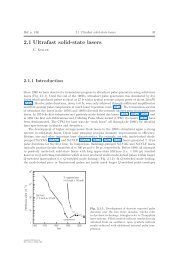
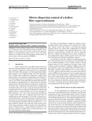
LASER PHYSICS IN THE LENGTH <strong>GAUGE</strong><br />
The length gauge (LG) has been favored since both the atomic binding potential and<br />
the laser field potential are scalars that can be added directly to provide a picture of<br />
the laser field “tilting” the Coulomb attractive field to result in a finite potential barrier<br />
that can be penetrated by the bound electron in a quantum tunneling event.<br />
V(r) = -1/r - Er<br />
1<br />
0<br />
-1<br />
-10 -5 0 5 10<br />
r<br />
23
QUALITATIVE IMPLICATIONS <strong>OF</strong> THE LENGTH <strong>GAUGE</strong><br />
The interaction Hamiltonian in the LG is simply r ∙ E (t) .<br />
This leads to simple implications.<br />
The fact that this H I connects continuously to the static-electric-field<br />
case has been regarded not merely as an advantage, but has been<br />
treated as a requirement.<br />
24
Intensity (a.u.)<br />
Intensity (W/cm 2 )<br />
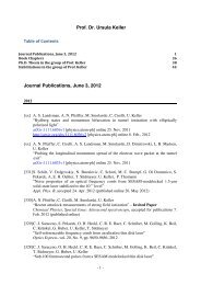
LASER PHYSICS VIEWED FROM THE LENGTH <strong>GAUGE</strong>: FIELD INTENSITY<br />
10 4<br />
10 3<br />
10 2<br />
10 1<br />
10 0<br />
10 -1<br />
10 -2<br />
10 -3<br />
10 -4<br />
Wavelength (nm)<br />
10 4 10 3 10 2 10 1<br />
10.6 m<br />
CO 2<br />
800 nm<br />
Ti:sapph<br />
Strong Fields<br />
Weak Fields<br />
Electric field = 1 a.u.<br />
100 eV<br />
10 -3 10 -2 10 -1 10 0 10 1<br />
Field frequency (a.u.)<br />
10 20<br />
10 19<br />
10 18<br />
10 17<br />
10 16<br />
10 15<br />
10 14<br />
10 13
Intensity (a.u.)<br />
Intensity (W/cm 2 )<br />
LASER PHYSICS VIEWED FROM THE LENGTH <strong>GAUGE</strong>: FIELD FREQUENCY<br />
The boundary between high and low frequency should be taken to be E B .<br />
10 4<br />
10 3<br />
10 2<br />
10 1<br />
10 0<br />
10 -1<br />
10 -2<br />
10 -3<br />
10 -4<br />
Wavelength (nm)<br />
10 4 10 3 10 2 10 1<br />
10.6 m<br />
CO 2<br />
Low<br />
Frequency<br />
800 nm<br />
Ti:sapph<br />
High<br />
Frequency<br />
100 eV<br />
10 -3 10 -2 10 -1 10 0 10 1<br />
Field frequency (a.u.)<br />
10 20<br />
10 19<br />
10 18<br />
10 17<br />
10 16<br />
10 15<br />
10 14<br />
10 13
QUALITATIVE IMPLICATIONS <strong>OF</strong> THE VELOCITY <strong>GAUGE</strong><br />
The solution of the Schrodinger equation in the VG connects<br />
continuously to the solution for an electron in a plane-wave field from<br />
the Dirac equation.<br />
This provides direct information on conditions for:<br />
• The boundary for the onset of non-dipole conditions: v/c effects.<br />
• The boundary for the onset of relativistic conditions: (v/c) 2 effects.<br />
Important: The dipole approximation fails at high frequencies where k∙r<br />
cannot be neglected, but it also fails at low frequencies where the<br />
coupling between electric and magnetic fields becomes important. This<br />
coupling can be visualized in terms of the motion of a free electron in a<br />
plane-wave field.<br />
Footnote: This was a surprise for the Joint Theoretical Physics Colloquium. They knew only of k∙r<br />
being neglected. That was a surprise to me.<br />
27
CLASSICAL FREE ELECTRON IN A PLANE WAVE FIELD<br />
Electron follows a figure-8 trajectory resulting from the combined action<br />
of the electric and magnetic fields.<br />
α 0 = amplitude along electric field direction<br />
β 0 = amplitude along direction of propagation<br />
α<br />
0<br />
<br />
c<br />
ω<br />
2z<br />
f<br />
,<br />
β<br />
0<br />
<br />
c<br />
ω<br />
zf<br />
4<br />
,<br />
β<br />
α<br />
0<br />
0<br />
<br />
1<br />
4<br />
zf<br />
2<br />
,<br />
z<br />
f<br />
<br />
2U<br />
mc<br />
p<br />
2
DOMAINS FOR AN ELECTRON IN A PLANE-WAVE FIELD<br />
Lasers produce plane-wave (PW) fields, not quasistatic (QSE) fields, so<br />
the beyond-dipole-approximation results in the VG have significance<br />
that the LG does not have.<br />
Specifically, the limits of relativistic effects and magnetic field effects<br />
shown on the next slide have real laboratory significance.<br />
Also shown is the upper limit on intensity for which perturbation theory<br />
is applicable. This follows from both a relativistic investigation [HRR, J.<br />
Math. Phys. 3, 387 (1962)] and a nonrelativistic investigation [HRR, Phys.<br />
Rev. A 22, 1786 (1980)].<br />
Most of what follows here was a surprise for the Joint Theoretical Physics Colloquium, including<br />
intensity-dependent failure of the dipole approximation.<br />
29
Intensity (a.u.)<br />
Intensity (W/cm 2 )<br />
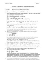
LASER PHYSICS VIEWED FROM THE COULOMB <strong>GAUGE</strong><br />
10 4<br />
10 3<br />
10 2<br />
10 1<br />
10 0<br />
10 -1<br />
10 -2<br />
10 -3<br />
10 -4<br />
Wavelength (nm)<br />
10 4 10 3 10 2 10 1<br />
10.6 m<br />
CO 2<br />
Relativistic<br />
2U p =mc 2<br />
Non-dipole<br />
800 nm<br />
Ti:sapph<br />
0 =1<br />
U p =<br />
Perturbative<br />
100 eV<br />
10 -3 10 -2 10 -1 10 0 10 1<br />
Field frequency (a.u.)<br />
10 20<br />
10 19<br />
10 18<br />
10 17<br />
10 16<br />
10 15<br />
10 14<br />
10 13<br />
limsVG 19apr10
VG-LG COMPARISON<br />
It has just been seen that VG and LG behaviors are completely different<br />
when a broad view is taken.<br />
Lasers produce plane waves, so the Coulomb gauge (VG in the dipole<br />
limit) is the physical gauge.<br />
However, because of gauge invariance, the LG can nevertheless give<br />
correct results for calculation of explicit laboratory-measurable<br />
quantities.<br />
The domain in which the LG (and all tunneling theories) can provide<br />
useful information is shown by the shaded area in the following slide<br />
from HRR, Phys. Rev. Lett 101, 043002 (2008).<br />
Footnote: An important property of this limited zone for the usefulness of tunneling<br />
methods is that a tunneling analysis in itself gives no hint of its own limited<br />
applicability.<br />
31
Intensity (a.u.)<br />
= 1/2<br />
Intensity (W/cm 2 )<br />
10 4<br />
10 3<br />
10 2<br />
10 1<br />
10 0<br />
10 -1<br />
10 -2<br />
10 -3<br />
10 -4<br />
Wavelength (nm)<br />
10 4 10 3 10 2 10 1<br />
10.6 m<br />
CO 2<br />
z f = 1 (2U p = mc 2 )<br />
0 = 1<br />
800 nm<br />
Ti:sapph<br />
100 eV<br />
10 -3 10 -2 10 -1 10 0 10 1<br />
Field frequency (a.u.)<br />
10 20<br />
10 19<br />
10 18<br />
10 17<br />
10 16<br />
10 15<br />
10 14<br />
10 13<br />
32
CONTRADICTIONS<br />
Much success has been achieved with the length gauge in general and<br />
tunneling ionization in particular, but according to what has been<br />
shown, the length gauge contradicts the result that the physical gauge<br />
is that gauge where transverse fields (laser fields) are represented by<br />
vector potentials A.<br />
Since tunneling ionization employs a non-physical gauge, “laboratory<br />
measurables” will be predicted correctly, but there should exist physical<br />
inconsistencies such as the failure of energy conservation in the classical<br />
static field example.<br />
What are the contradictions<br />
associated with tunneling?<br />
33
INCORRECT PREDICTIONS FROM TUNNELING THEORY<br />
• A laser field is strong when the electric field is of the order of one<br />
atomic unit; that is, when the external field is of the order of magnitude<br />
of internal fields in the atom. (Already examined.)<br />
• A single parameter – the Keldysh parameter γ – is sufficient for scaling.<br />
• Weak fields can be characterized as in the multiphoton domain and<br />
strong fields are in the tunneling domain.<br />
• A tunneling limit or classical limit will be approached at long<br />
wavelengths of the field.<br />
• There are no evident upper and lower frequency limits on the dipole<br />
approximation.<br />
• Higher harmonics are not produced by circularly polarized fields<br />
because the photoelectron “walks away” from the atom.<br />
34
PONDEROMOTIVE ENERGY<br />
A charged particle in a plane-wave field has a minimal interaction energy with the<br />
field. That is, even a particle at rest on average has a minimal interaction energy with<br />
the field (sometimes called “quiver energy”). This is the ponderomotive energy U p .<br />
KELDYSH GAMMA PARAMETER<br />
Based on the tunneling concept, the following classification is nearly universal in the<br />
strong-field community:<br />
35
PROBLEMS ASSOCIATED WITH THE KELDYSH PARAMETER<br />
If the binding energy is set at E B = 0.5 a.u. (ground-state hydrogen), then<br />
I<br />
<br />
( / )<br />
2<br />
Plotted as I vs. , this produces the following simple diagram that<br />
completely contradicts the “standard tunneling / multiphoton”<br />
classification.<br />
36
Intensity (a.u.)<br />
Intensity (W/cm 2 )<br />
10 7<br />
10 6<br />
10 5<br />
10 4<br />
10 3<br />
10 2<br />
10 1<br />
10 0<br />
10 -1<br />
10 -2<br />
10 -3<br />
10 -4<br />
Wavelength (nm)<br />
10 4 10 3 10 2 10 1<br />
10.6 m<br />
CO 2<br />
E=1a.u.<br />
800 nm<br />
Ti:sapph<br />
= 0.1<br />
= 1.0<br />
= 10<br />
10 -3 10 -2 10 -1 10 0 10 1<br />
Field frequency (a.u.)<br />
100 eV<br />
10 23<br />
10 22<br />
10 21<br />
10 20<br />
10 19<br />
10 18<br />
10 17<br />
10 16<br />
10 15<br />
10 14<br />
10 13<br />
A fixed value of cannot distinguish “tunneling” from “multiphoton”. = 0.1 is<br />
supposedly “tunneling”, but the right-hand end of this line is at 10 a.u. = 272 eV.<br />
37
ANOTHER DEFECT <strong>OF</strong> THE LG/TUNNELING VIEWPOINT<br />
The limit 0 is regarded as the “tunneling limit”, which is identified<br />
as the static limit, which is unquestionably tunneling – if that were the<br />
correct limit.<br />
However, the next figure shows that, viewed as a plane wave (i.e. a laser<br />
field), 0 is actually an extreme relativistic limit.<br />
38
Intensity (a.u.)<br />
Intensity (W/cm 2 )<br />
10 7<br />
10 6<br />
10 5<br />
10 4<br />
10 3<br />
10 2<br />
10 1<br />
10 0<br />
10 -1<br />
10 -2<br />
10 -3<br />
10 -4<br />
Wavelength (nm)<br />
10 4 10 3 10 2 10 1<br />
10.6 m<br />
CO 2<br />
0<br />
= 0.001<br />
= 0.01<br />
Relativistic Domain<br />
800 nm<br />
Ti:sapph<br />
z f = 1 (2U p = mc 2 )<br />
= 0.1<br />
= 1<br />
100 eV<br />
E=1a.u.<br />
10 -3 10 -2 10 -1 10 0 10 1<br />
Field frequency (a.u.)<br />
10 23<br />
10 22<br />
10 21<br />
10 20<br />
10 19<br />
10 18<br />
10 17<br />
10 16<br />
10 15<br />
10 14<br />
10 13<br />
The line at 2U p = mc 2 is where the minimum interaction energy of an electron with the laser<br />
field is of the order of the rest energy of the electron. The left / upper corner of the graph is an<br />
extreme relativistic zone. Laser-induced ionization is not a static limit.<br />
39
THE CAUSE <strong>OF</strong> THIS FUNDAMENTAL PROBLEM<br />
The length gauge is NOT the physical gauge for laser-induced<br />
phenomena.<br />
The Coulomb gauge IS the physical gauge.<br />
The tunneling picture (LG picture) is completely erroneous when used<br />
outside the limited domain where there is a gauge equivalence to the<br />
Coulomb gauge (VG).<br />
Within the gauge equivalence domain, the LG can give correct answers<br />
for physical measurables, but its qualitative inferences are seriously in<br />
error.<br />
This simple error has led astray an entire community of<br />
very smart people.<br />
40
ANOTHER FUNDAMENTAL PROBLEM<br />
The ponderomotive energy U p is a fundamental quantity in strong-field physics. (It<br />
does not appear in any finite order of perturbation theory – but that is a different<br />
interesting story.)<br />
The ponderomotive energy can be such that<br />
U<br />
p<br />
E<br />
B<br />
even within the domain where the dipole approximation is valid.<br />
In atomic units,<br />
U p<br />
<br />
where the angle bracket means a time average over a full period. Within the dipole<br />
approximation,<br />
1<br />
2<br />
A<br />
c<br />
2<br />
A A<br />
2 ( t) U U ( t)<br />
2<br />
p<br />
p<br />
41
The problem is that U p is absolutely basic in strong fields, it can be large, but there is<br />
an elementary theorem in classical mechanics that any quantity that is solely a<br />
function of time can be removed from the Hamiltonian without consequences.<br />
(This is obvious from the Hamilton equations of motion.)<br />
If U p is removed, strong-field physics gives wrong answers. What is going on?<br />
The answer to this paradox can be found in a classical – quantum distinction.<br />
In classical physics, measurements are direct; in quantum physics, measurements are<br />
not made inside the interaction region, they are made outside that region.<br />
That means that measurements are indirect in quantum mechanics; if an f(t) function<br />
is removed inside the region it causes an unphysical shift with respect to the<br />
measuring instruments. If that shift is a function of the vector potential, it is<br />
meaningless to remove it for the measuring instruments, which know nothing of laser<br />
fields. Hence, it cannot be removed within the interaction region.<br />
42
RIGOROUS DERIVATION <strong>OF</strong> AN S MATRIX<br />
Basic requirement: The transition-causing interaction occurs only within a domain<br />
bounded in space and time.<br />
(Example: transitions in the focus of a pulsed laser.)<br />
Important properties of an S matrix as derived here:<br />
‣ It can be formulated entirely in terms of quantities measurable in<br />
the laboratory.<br />
‣ It does not require that dynamics be tracked over time. Equations of<br />
motion are incorporated in the S matrix.<br />
‣ There is no need for “adiabatic decoupling”.<br />
‣ It gives unambiguous rules for gauge transformations.<br />
‣ It can be applied to any process as long as the space-time domain of<br />
the interaction region is bounded.<br />
43
The general problem is evoked of an atomic electron subjected to a<br />
pulsed, focused laser beam. This is a convenience, not a requirement.<br />
There will be a complete set of states { n } that satisfy the Schrödinger equation<br />
describing the atomic electron that may be undisturbed or in interaction with a laser<br />
beam:<br />
it<br />
H<br />
The outcome of any experiment will be measured by laboratory<br />
instruments that never experience a laser field. As far as the laboratory<br />
instruments are concerned, there is a complete set of states { n } that<br />
satisfy the Schrödinger equation describing an atomic electron that does<br />
NOT experience the laser field:<br />
i<br />
H0<br />
t<br />
44
By hypothesis, the laser pulse is finite, so<br />
H<br />
t<br />
H 0<br />
lim<br />
0 <br />
t<br />
We can organize the two complete sets of states and states so that they<br />
correspond at t - :<br />
lim<br />
t<br />
<br />
t<br />
t<br />
0<br />
n<br />
After the laser interaction has occurred, the only way for the laboratory instruments to<br />
discover what has happened is to form overlaps of all possible final f states with the<br />
state that began as a particular i state. This is the S matrix:<br />
S<br />
fi<br />
<br />
lim<br />
t<br />
<br />
<br />
n<br />
f<br />
, <br />
Subtract the amplitude that no transition has occurred:<br />
i<br />
<br />
M<br />
fi<br />
<br />
S<br />
1<br />
lim <br />
, <br />
lim <br />
, <br />
fi<br />
t<br />
f<br />
i<br />
t<br />
f<br />
i<br />
45
We now have the form of a perfect differential:<br />
<br />
Mfi<br />
dt <br />
f<br />
, i<br />
<br />
<br />
t<br />
M<br />
M<br />
M<br />
M<br />
fi<br />
fi<br />
fi<br />
fi<br />
<br />
<br />
<br />
<br />
<br />
<br />
<br />
<br />
i<br />
<br />
t<br />
i<br />
<br />
t<br />
<br />
<br />
<br />
<br />
i<br />
<br />
dt<br />
<br />
, <br />
<br />
, <br />
<br />
H<br />
H <br />
<br />
iH<br />
H <br />
dt<br />
dt<br />
<br />
<br />
0<br />
0<br />
t<br />
<br />
iH , <br />
<br />
, iH<br />
H <br />
i<br />
<br />
,H <br />
i<br />
, H<br />
H <br />
<br />
f<br />
f<br />
f<br />
0<br />
0<br />
dt ,H <br />
i<br />
H iH<br />
<br />
I<br />
t<br />
f<br />
I<br />
i<br />
i<br />
An alternative form is especially useful for strong-field problems. Instead of making a<br />
one-to-one correspondence of and states at t - , do it at t + and then<br />
look for the probabilities that particular initial states could have led to this final result.<br />
i<br />
<br />
f<br />
t<br />
f<br />
t<br />
0<br />
f<br />
i<br />
0<br />
0<br />
0<br />
I<br />
I<br />
<br />
i<br />
I<br />
<br />
<br />
<br />
i<br />
<br />
46
The end result of this alternative procedure is the transition matrix element<br />
M<br />
fi<br />
<br />
i<br />
<br />
dt<br />
<br />
<br />
f<br />
, H<br />
I<br />
<br />
i<br />
<br />
The first form above is called the direct-time S matrix, and the second form is the time-reversed<br />
S matrix.<br />
In general, states are known exactly or can be simulated accurately (for example, by analytical<br />
Hartree-Fock procedures). It is the states that present the problem because they represent<br />
conditions for an electron simultaneously subjected to the Coulomb attraction and to the laser<br />
field. No exact solutions are known.<br />
If the initial state i is to be approximated, this is very difficult because the laser field (by<br />
hypothesis) is too strong to be treated perturbatively, and so is the Coulomb field because in an<br />
initial bound state the Coulomb field has a singularity at the origin.<br />
For the final state f , the electron is unbound, and the laser field can be assumed to be more<br />
important than the Coulomb field. This identifies the time-reversed S matrix as the preferred<br />
form, and it will be employed exclusively hereafter.<br />
47
<strong>GAUGE</strong> TRANSFORMATIONS ARE NOT UNITARY<br />
It is widely known and easily shown that a gauge transformation applied to the<br />
Schrödinger equation gives the result<br />
( H i )' U( H i<br />
) U <br />
t<br />
where U is the unitary operator that generates the gauge transformation. Although it is true that<br />
' U<br />
in order to have form invariance of the Schrödinger equation, the first equation above<br />
will not give the unitary transformation of operators<br />
1<br />
O ' UOU <br />
if U is time-dependent.<br />
The above is a rebuttal to the statement in the Preamble:<br />
• A gauge transformation is a unitary transformation.<br />
t<br />
1<br />
48
TRANSITION MATRIX ELEMENTS ARE NOT MANIFESTLY <strong>GAUGE</strong> INVARIANT<br />
In AMO papers and textbooks, one commonly finds the statement that quantum<br />
transition amplitudes are manifestly gauge invariant. This is justified by the expression<br />
That is an expression for a change of quantum picture, not for a gauge transformation.<br />
In a gauge transformation, field-dependent quantities change, the non-interacting<br />
reference states do not change. In a gauge transformation<br />
Demonstrating gauge invariance is nontrivial.<br />
The above is a rebuttal to the statement in the Preamble:<br />
• Quantum transition amplitudes are manifestly gauge invariant.<br />
49
A FUNCTION <strong>OF</strong> TIME ONLY f(t), CAN BE REMOVED BY A <strong>GAUGE</strong> TRANSFORMATION<br />
This is not the same as simply dropping a function of time. A gauge transformation<br />
should, under appropriate conditions, make it possible to calculate laboratory<br />
measurables.<br />
The ponderomotive energy can be the cause of “channel closings”, and also the cause<br />
of “high-frequency stabilization”. These are physically important effects. A dilemma<br />
appears to remain.<br />
The simplest case to consider is the stabilization matter. “Stabilization” is that property<br />
of strong-field phenomena where, beyond a certain field intensity, further increases in<br />
intensity lead to a decline in the transition rate rather than an increase.<br />
The next figures [from HRR, J. Opt. Soc. Am. B 13, 355 (1996)] show the results of<br />
calculating with the SFA (Strong-Field Approximation) and the HFA (High Frequency<br />
Approximation). The stabilization occurs at about the same intensity with both<br />
methods, but A 2 (t) is included in the SFA, and it has been removed by a gauge<br />
transformation in the HFA.<br />
50
The SFA includes A 2 (t); the HFA has removed that term by a gauge transformation.<br />
51
EXPLANATION<br />
Because the frequency is high ( >> E B ), the ionization process takes<br />
place at low intensities with a single photon. In the SFA, the stabilization<br />
occurs because the ponderomotive energy has become so large as a<br />
result of increasing the field strength that the single-photon channel has<br />
closed and at least two photons are required for ionization.<br />
There are no channel closings in the HFA because A 2 (t) has been<br />
removed by a gauge transformation. The physical explanation for why<br />
stabilization has occurred has changed (there is no simple explanation in<br />
the HFA), but gauge equivalence preserves the physical effect.<br />
This is another example (beyond tunneling) where the physical<br />
explanation is dependent on the gauge even when gauge equivalence<br />
leads to the same predicted result.<br />
52
REVISIT ITEMS FROM THE PREAMBLE<br />
• Physical processes involving electromagnetic interactions depend entirely on the electric and<br />
magnetic fields that are present.<br />
Physical processes depend on potentials as well as fields. See the first example of the constant<br />
electric field.<br />
• These fields can be represented as derivatives of scalar and vector potential functions that are<br />
often mathematically convenient, but are actually only auxiliary quantities.<br />
Potentials play a more fundamental role than just being “auxiliary quantities”.<br />
• The potential functions are not unique. There are many sets of these functions corresponding<br />
to the same fields and thus to the same physical processes.<br />
Different gauges can correspond to the same fields, but not to the same physical processes. The<br />
stabilization example is very clear on this point.<br />
53
• The choice of which of the possible sets of potentials to use for a given problem is a matter of<br />
mathematical or conceptual convenience.<br />
“Mathematical” perhaps. “Conceptual” no.<br />
• Exactly the same considerations about the choice of gauge apply to both classical and quantum<br />
phenomena.<br />
Quantum phenomena differ from classical in that laboratory measurements are indirect.<br />
All of the questionable (although widely accepted) remarks in the Preamble have been<br />
addressed except the very last one:<br />
• The most basic approach is to formulate all problems using a scalar potential. (Within the<br />
dipole approximation, this is called the length gauge.) If a different gauge is desired, this should<br />
be obtained through a gauge transformation from the length gauge.<br />
This is transparently false. It is not possible to infer the 4-vector A from a scalar potential .<br />
Nevertheless, there is a considerable literature bearing some well-known names that accept this<br />
assertion.<br />
54