2.1 Ultrafast solid-state lasers - ETH - the Keller Group

122 2.1.7 Pulse characterization [Ref. p. 134
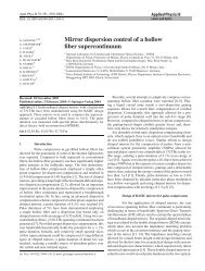
Table 2.1.13. Optical pulses: defining equations for Gaussian and soliton pulse shapes, FWHM (fullwidth-half-maximum)
intensity pulse duration τ p, time–bandwidth products Δν pτ p for which Δν p is the
FWHM of the spectral intensity, FWHM intensity autocorrelation pulse duration τ Au.
Pulse shape τ p/τ Δν pτ p τ p/τ Au
( ) t
2
Gauss: I (t) ∝ exp
2 √ ln 2 0.4413 0.7071
τ 2
Soliton: I (t) ∝ sech 2 ( t
τ
)
1.7627 0.3148 0.6482
example, that allow for parabolic approximation of pulse-formation mechanisms one expects a
sech 2 temporal and spectral pulse shape (Sects. 2.1.6.4–2.1.6.7). Passively mode-locked solid-state
lasers with pulse durations well above 10 fs normally generate pulses close to this ideal sech 2 -
shape. Therefore, this non-collinear autocorrelation technique is a good standard diagnostic for
such laser sources. For ultrashort pulse generation in the sub-10-fs regime this is generally not the
case anymore. Experimentally, this is clearly indicated by more complex pulse spectra.
Interferometric AutoCorrelation (IAC) techniques [83Min] have been used to get more information.
In IAC a collinear intensity autocorrelation is fringe-resolved and gives some indication
how well the pulse is transform-limited. However, we still do not obtain full phase information
about the pulse. The temporal parameters have usually been obtained by fitting an analytical
pulse shape with constant phase to the autocorrelation measurement. Theoretical models of the
pulse-formation process motivate the particular fitting function. For lasers obeying such a model
the a-priori assumption of a theoretically predicted pulse shape is well-motivated and leads to
good estimates of the pulse duration as long as the measured spectrum also agrees with the theoretical
prediction. However, we have seen that fits to an IAC trace with a more complex pulse
spectrum tend to underestimate the true duration of the pulses. Problems with IAC measurement
for ultrashort pulses are also discussed in the two-optical-cycle regime [04Yam].
For few-cycle pulses, a limitation in a noncollinear beam geometry arises because of the finite
crossing angle of two beams. In this case the temporal delay between two beams is different in the
center and in the wings of the spatial beam profile. This geometrical artifact results in a measured
pulse duration that is longer than the actual pulse duration τ p :
τ 2 p,meas = τ 2 p + δτ 2 . (2.1.85)
For a beam diameter d and a crossing angle θ betweenthetwobeamsthisresultsinanδτ of
δτ = √ 2 d c tan θ 2 ≈
θd √
2 c
(2.1.86)
with the speed of light c and the additional approximation for a small crossing angle θ. For example
a crossing angle of 1.7 ◦ and a beam diameter of 30 μm results in δτ =2.1 fs. For an actual
pulse duration of 10 fs (resp. 5 fs) this gives a measured pulse duration of 10.2 fs (resp. 5.4 fs)
which corresponds to an error of 2 % (resp. 8 %). This means this becomes more severe for pulse
durations in the few-cycle regime. However, if the crossing angle is significantly increased this
can become also more important for longer pulses. For this reason, in the few-cycle-pulse-width
regime collinear geometries have always been preferred to avoid geometrical blurring artifacts and
to prevent temporal resolution from being reduced.
Landolt-Börnstein
New Series VIII/1B1