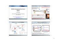
2.1 Ultrafast solid-state lasers - ETH - the Keller Group
2.1 Ultrafast solid-state lasers - ETH - the Keller Group
2.1 Ultrafast solid-state lasers - ETH - the Keller Group

Create successful ePaper yourself
Turn your PDF publications into a flip-book with our unique Google optimized e-Paper software.
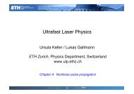
108 <strong>2.1</strong>.6 Mode-locking techniques [Ref. p. 134<br />
A (z,t) =e −iδL|A(t)|2 A (0,t)e −ikn(ω0)z ≈<br />
After one cavity round trip we <strong>the</strong>n obtain<br />
(<br />
1 − iδ L |A (t)| 2) A (0,t)e −ikn(ω0)z . (<strong>2.1</strong>.46)<br />
ΔA ≈−iδ L |A| 2 A. (<strong>2.1</strong>.47)<br />
<strong>2.1</strong>.6.3 Active mode-locking<br />
Short pulses from a laser can be generated with a loss or phase modulator inside <strong>the</strong> resonator.<br />
For example, <strong>the</strong> laser beam is amplitude-modulated when it passes through an acousto-optic<br />
modulator. Such a modulator can modulate <strong>the</strong> loss of <strong>the</strong> resonator at a period equal to <strong>the</strong><br />
round-trip time T R of <strong>the</strong> resonator (i.e. fundamental mode-locking). The pulse evolution in an<br />
actively mode-locked laser without Self-Phase Modulation (SPM) and <strong>Group</strong>-Velocity Dispersion<br />
(GVD) can be described by <strong>the</strong> master equation of Haus [75Hau2]. Taking into account gain<br />
dispersion and loss modulation we obtain with (<strong>2.1</strong>.32) and (<strong>2.1</strong>.34) (Table <strong>2.1</strong>.10) <strong>the</strong> following<br />
differential equation:<br />
∑<br />
ΔA i =<br />
i<br />
[<br />
g<br />
(<br />
1+ 1 Ω 2 g<br />
∂ 2 )<br />
∂t 2 − l − M ω mt 2 ]<br />
A (T,t)=0. (<strong>2.1</strong>.48)<br />
2<br />
Typically we obtain pulses which are much shorter than <strong>the</strong> round-trip time in <strong>the</strong> cavity and<br />
which are placed in time at <strong>the</strong> position where <strong>the</strong> modulator introduces <strong>the</strong> least amount of loss.<br />
Therefore, we were able to approximate <strong>the</strong> cosine modulation by a parabola (<strong>2.1</strong>.33). The only<br />
stable solution to this differential equation is a Gaussian pulse shape with a pulse duration:<br />
τ p =1.66 × 4 √D g /M s , (<strong>2.1</strong>.49)<br />
where D g is <strong>the</strong> gain dispersion ((<strong>2.1</strong>.32) and Table <strong>2.1</strong>.10) and M s is <strong>the</strong> curvature of <strong>the</strong> loss<br />
modulation ((<strong>2.1</strong>.33) and Table <strong>2.1</strong>.10). Therefore, in active mode-locking <strong>the</strong> pulse duration becomes<br />
shorter until <strong>the</strong> pulse shortening of <strong>the</strong> loss modulator balances <strong>the</strong> pulse broadening of <strong>the</strong><br />
gain filter. Basically, <strong>the</strong> curvature of <strong>the</strong> gain is given by <strong>the</strong> gain dispersion D g and <strong>the</strong> curvature<br />
of <strong>the</strong> loss modulation is given by M s . The pulse duration is only scaling with <strong>the</strong> fourth root of<br />
<strong>the</strong> saturated gain (i.e. τ p ∝ 4√ g) and <strong>the</strong> modulation depth (i.e. τ p ∝ 4√ 1/M ) and with <strong>the</strong> square<br />
root of <strong>the</strong> modulation frequency (i.e. τ p ∝ √ 1/ω m ) and <strong>the</strong> gain bandwidth (i.e. τ p ∝ √ 1/Δ ω g ).<br />
A higher modulation frequency or a higher modulation depth increases <strong>the</strong> curvature of <strong>the</strong> loss<br />
modulation and a larger gain bandwidth decreases gain dispersion. Therefore, we obtain shorter<br />
pulse durations in all cases. At steady <strong>state</strong> <strong>the</strong> saturated gain is equal to <strong>the</strong> total cavity losses,<br />
<strong>the</strong>refore, a larger output coupler will result in longer pulses. Thus, higher average output power<br />
is generally obtained at <strong>the</strong> expense of longer pulses (Table <strong>2.1</strong>.2).<br />
The results that have been obtained in actively mode-locked flashlamp-pumped Nd:YAG and<br />
Nd:YLF <strong>lasers</strong> can be very well explained by this result. For example, with Nd:YAG at a lasing<br />
wavelength of 1.064 μm we have a gain bandwidth of Δλ g =0.45 nm. With a modulation frequency<br />
of 100 MHz (i.e. ω m =2π·100 MHz), a 10 % output coupler (i.e. 2g ≈ T out =0.1) and a modulation<br />
depth M =0.2, we obtain a FWHM pulse duration of 93 ps (<strong>2.1</strong>.49). For example, with Nd:YLF<br />
at a lasing wavelength of 1.047 μm and a gain bandwidth of Δλ g =1.3 nmweobtainwith<strong>the</strong><br />
same mode-locking parameters a pulse duration of 53 ps (<strong>2.1</strong>.49).<br />
The same result for <strong>the</strong> pulse duration (<strong>2.1</strong>.49) has been previously derived by Kuizenga and<br />
Siegman [70Kui1, 70Kui2] where <strong>the</strong>y assumed a Gaussian pulse shape and <strong>the</strong>n followed <strong>the</strong><br />
pulse once around <strong>the</strong> laser cavity, through <strong>the</strong> gain and <strong>the</strong> modulator. They <strong>the</strong>n obtained a<br />
self-consistent solution when no net change occurs in <strong>the</strong> complete round trip. The advantage of<br />
Landolt-Börnstein<br />
New Series VIII/1B1