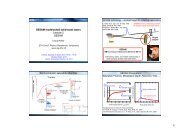
2.1 Ultrafast solid-state lasers - ETH - the Keller Group

106 2.1.6 Mode-locking techniques [Ref. p. 134
and
∂ 2
{
∂2 1
A (t) =
∂t2 ∂t 2 2π
∫
}
à (ω)e iΔωt dω = 1 ∫
2π
à (ω) [ −Δω 2] e iΔωt dω. (2.1.31)
For the change in the pulse envelope ΔA = A out − A in after the gain medium we then obtain:
∂
ΔA ≈
[g 2 ]
+ D g
∂t 2 A, D g ≡ g Ωg
2
, (2.1.32)
where D g is the gain dispersion.
2.1.6.2.2 Loss modulator
A loss modulator inside a laser cavity is typically an acousto-optic modulator and produces a
sinusoidal loss modulation given by a time-dependent loss coefficient:
l (t) =M (1 − cos ω m t) ≈ M s t 2 , M s ≡ Mω2 m
, (2.1.33)
2
where M s is the curvature of the loss modulation, 2M is the peak-to-peak modulation depth and
ω m the modulation frequency which corresponds to the axial mode spacing in fundamental modelocking.
In fundamental mode-locking we only have one pulse per cavity round trip. The change
in the pulse envelope is then given by
A out (t) =e −l(t) A in (t) ≈ [1 − l (t)] A in (t) ⇒ ΔA ≈−M s t 2 A. (2.1.34)
2.1.6.2.3 Fast saturable absorber
In case of an ideal fast saturable absorber we assume that the loss recovers instantaneously and
therefore shows the same time dependence as the pulse envelope, (2.1.17) and (2.1.18):
q (t) =
q 0
q 0
≈ q 0 − γ A P (t) , γ A ≡ . (2.1.35)
1+I A (t)/I sat,A I sat,A A A
The change in the pulse envelope is then given by
A out (t) =e −q(t) A in (t) ≈ [1 − q (t)] A in (t) ⇒ ΔA ≈ γ A |A| 2 A. (2.1.36)
2.1.6.2.4 Group velocity dispersion (GVD)
Thewavenumberk n (ω) in a dispersive material depends on the frequency and can be approximately
written as:
k n (ω) ≈ k n (ω 0 )+k nΔ ′ ω + 1 2 k′′ nΔ ω 2 + ... , (2.1.37)
where Δ ω = ω − ω 0 , k n ′ = ∂k ∣
n
∂ω ∣ and k n ′′ = ∂2 k n ∣∣∣ω=ω0
ω=ω0
∂ω 2 . In the frequency domain the pulse
envelope in a dispersive medium after a propagation distance of z is given by
à (z,ω) =e −i[kn(ω)−kn(ω0)]z à (0,ω) ≈{1 − i[k n (ω) − k n (ω 0 )] z} à (0,ω) , (2.1.38)
Landolt-Börnstein
New Series VIII/1B1