A Study of the MIMO Channel Capacity When Using the Geometrical ...

A STUDY OF THE MIMO CHANNEL CAPACITY WHEN
USING THE GEOMETRICAL TWO-RING SCATTERING MODEL
Bjørn Olav Hogstad and Matthias Pätzold
Department of Information and Communication Technology
Faculty of Engineering and Science, Agder University College
Grooseveien 36, NO-4876 Grimstad, Norway
E-mail: bjorn.o.hogstad@hia.no
Abstract— In this paper, analytical and simulation results for the
capacity of multiple-input multiple-output (MIMO) channels are presented.
Our study has been performed by using the so-called tworing
scattering model. The underlying geometrical model consists of
local scatterers laying on two separated rings around the base station
(BS) and the mobile station (MS). It is assumed that the scatterers
are located on the two rings according to the von Mises distribution.
Both the spatial and temporal correlation of the channel are taken
into account. Approximate second order moments of the channel
eigenvalues are studied. It is shown that the approximation converges
to the true moments of the eigenvalues as either the number of BS or
MS antennas tends to infinity. Simulations indicate that this is also true
for realistic array sizes. A new tight upper bound on the 2 × 2 MIMO
channel capacity is derived. Furthermore, simulation results for the
level crossing rate (LCR) of the channel capacity are presented.
Keywords: MIMO channel capacity, asymptotic analysis, eigenvalue
distribution, space-time correlation, MIMO channel modelling.
1. INTRODUCTION
Multiple-input multiple-output (MIMO) channels have multiple
antennas at both the transmit and receive side. Under favorable
propagation conditions, the channel capacity—the maximum rate
at which data can be transmitted without errors—has shown to
increase proportionally to the minimum number of antennas at
the transmitter and receiver [1], [2]. However, under real-world
conditions, the MIMO channel capacity may be limited due to
several factors. For example, it has been shown in [3] and [4] that
the correlation between the sub-channels has a strong influence on
the channel capacity. Therefore, MIMO channel models have been
developed recently, e.g., [5]–[9], where the spatial and temporal
correlations are accurately modelled under certain assumptions.
In this paper, we analyze and simulate the capacity by using the
stochastic MIMO channel simulation model proposed in [7] for the
two-ring model. We consider only a single cluster of scatterers on
each ring, although the simulation model can easily be extended
to include several clusters. Numerical computations of the mean
channel capacity can be very time consuming, especially when the
number of antenna elements at the transmit and/or receive side is
very large. In this paper, we have used the simple approximation
from [10] to predict the mean capacity. This approximation is based
on the channel eigenvalues, which will be studied in this paper for
the two-ring model.
A general upper bound on the mean channel capacity, which
is not limited to a particular scenario and accounts for both the
transmit and receive end correlations, can be found in [11]. In case
of the two-ring scattering model, a new tighter upper bound on the
mean capacity of a 2 × 2 MIMO channel is presented. The upper
bounds will be compared with the simulated mean capacity.
We will also give simulation results for the LCR of the MIMO
channel capacity. Here, the LCR of the capacity describes the
average number of up-crossings (or down-crossings) of the capacity
through a fixed level within one second. Since analytical solutions
for the LCR of the channel capacity do not exist, we believe that
the proposed MIMO channel simulator in [7] is quite useful for
determining this important quantity.
The remainder of this paper is organized as follows. Section II reviews
briefly the geometrical two-ring scattering model. We present
the stochastic MIMO channel simulation model in Section III. The
MIMO channel capacity is studied analytically in Section IV, and
the corresponding simulations results are presented in Section V.
Finally, the conclusions are drawn in Section VI.
2. THE GEOMETRICAL TWO-RING SCATTERING
MODEL
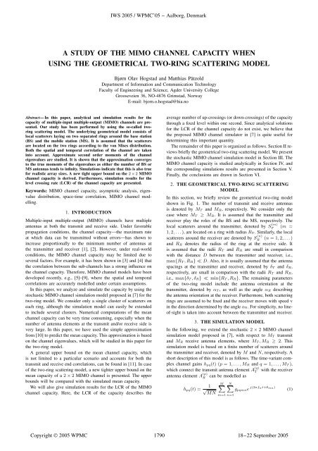
In this section, we briefly review the geometrical two-ring model
shown in Fig. 1. The number of transmit and receive antennas
is denoted by M T and M R, respectively. We consider only the
case where M T ≥ M R. It is assumed that the transmitter and
receiver play the roles of the BS and the MS, respectively. The
local scatterers around the transmitter, denoted by S (m)
T
(m =
1, 2,...), are located on a ring with radius R T . Similarly, the local
scatterers around the receiver are denoted by S (n)
R
(n =1, 2,...)
and R R denotes the radius of the ring at the receive side. It
is assumed that the radii R T and R R are small in comparison
with the distance D between the transmitter and receiver, i.e.,
max{R T ,R R}≪D. Also, it is usually assumed that the antenna
spacings at the transmitter and receiver, denoted by δ T and δ R,
respectively, are small in comparison with the radii R T and R R,
i.e., max{δ T ,δ R}≪min{R T ,R R}. The remaining parameters
of the two-ring model include the antenna orientation at the
transmitter, denoted by α T , as well as the angle α R describing
the antenna orientation at the receiver. Furthermore, both scattering
rings are assumed to be fixed and the receiver moves with speed v
in the direction determined by the angle αv. For simplicity, no lineof-sight
is taken into account between the transmitter and receiver.
3. THE SIMULATION MODEL
In the following, we extend the stochastic 2 × 2 MIMO channel
simulation model proposed in [7], with respect to M T transmit
and M R receive antenna elements, where M T ,M R ≥ 2. This
simulation model is based on a finite number of scatterers around
the transmitter and receiver, denoted by M and N, respectively. A
short description of this model is as follows. The time-variant complex
channel gains h pq(t) (p =1,...,M R and q =1,...,M T ),
which connect the transmit antenna element A (q)
T
with the receiver
antenna element A (p)
R
can be modelled as
h pq(t) =
1
√
MN
M
N
m=1 n=1
g pqmne j(2πfnt+θmn) (1)

y
A (1)
T
d 1m
α T
S (m)
T
d mn
d n2
S (n)
R
d n1
φ (n)
R
αv A (1)
R
δ T
φ (m)
T
α R
0 T 0 R δ R
d 2m
A (M R )
R
A (M T )
T
R T D
R R
Fig. 1. Geometrical model (two-ring model) for an M T × M R channel
with local scatterers around both the BS and MS.
where
g pqmn = a mq b np c mn (2)
a mq = e j(M T −2q+1)π(δ T /λ) cos(φ (m)
T −β T )
(3)
b np = e j(M R−2p+1)π(δ R /λ) cos(φ (n)
R −β R)
(4)
c mn = e j 2π λ (R T cos φ (m)
T
−R R cos φ (n)
R ) (5)
f n = f max cos(φ (n)
R
− αv) . (6)
The two sets {φ (m)
T
}M m=1 and {φ (n)
R
}N n=1 denote the angle of departure
(AOD) and angle of arrival (AOA), respectively. Furthermore,
the quantities f max and λ are denoting the maximum Doppler
frequency and the wavelength, respectively. Finally, the phases
θ mn are independent identically distributed random variables, each
with a uniform distribution over (0, 2π]. Note that the complex
channel gains h pq(t) are independent of the distance D between
the transmitter and receiver.
The space-time cross correlation function (CCF) of the stochastic
simulation model can be expressed as [7]
ρ(δ T ,δ R,τ)=ρ T (δ T ) · ρ R(δ R,τ). (7)
In [7], ρ T (δ T ) and ρ R(δ R,τ) are the transmit and receive correlation
functions, respectively, where the quantity τ denotes the time
lag. For the intention of the paper, we need the elements R T ij of
the M T × M T transmit correlation matrix R T =[R T ij], which can
be determined as follows
R T ij =
1
= 1 M
k=1
M
M R
M R
m=1
E{h ki (t)h ∗ kj(t)}
a m,2(j−i) (8)
where i, j =1,...,M T . The operators E{·} and (·) ∗ denote the
expectation and the complex conjugation, respectively. Similarly,
the elements R R ij of the M R×M R receive correlation matrix R R =
[R R ij] can be expressed as
R R ij =
= 1 N
1
M
T
N
M T
k=1
n=1
E{h ik (t)h ∗ jk(t)}
b n,2(j−i) (9)
where i, j =1,...,M R.Accordingto[7]wehaveR11 T = ρ T (δ T )
and R11
R = ρ R(δ R, 0). It should be mentioned that separable
transmit and receive antenna correlations where also used in [6],
x
[12], [13], and [14]. For the one-ring model, however, the spacetime
CCF is non-separable [13, 3].
For the space-time CCF given in (7), we need the distributions
p(φ T ) and p(φ R) of the AOD and AOA, respectively. In many
previous papers, such as [5], [15], and [6], the von Mises distribution
has been proposed to describe these distributions. The von
Mises distribution function is given by
1
p(φ) =
2πI 0(κ) eκ cos(φ−µ) , φ ∈ (0, 2π] (10)
where I 0(·) is the zeroth-order modified Bessel function, and
µ ∈ (0, 2π] accounts for the mean direction of the AOD/AOA.
The quantity κ ≥ 0 is a control parameter for the spread of the
scatterers. We denote κ T and κ R as the degree of local scattering
at the transmitter and receiver, respectively. Similarly, we define
µ T and µ R as the mean AOD and the mean AOA, respectively.
In case of isotropic scattering (κ T = κ R =0),wherep(φ T )=
p(φ R)=1/(2π), theAOD{φ (m)
T
}M m=1 and the AOA {φ (n)
R }N n=1
of the simulation model determined by (1) can be computed by
using the extended method of exact Doppler spread (MEDS) [7].
On the other hand, if we consider non-isotropic scattering at
either the transmit or receive side, we recommend to compute the
parameters {φ (m)
T
}M m=1 or {φ (n)
R
}N n=1 according to a variant of the
L p-norm method described in [7].
4. THE MIMO CHANNEL CAPACITY
In this section, we study the information-theoretic channel capacity
C(t), in bits/s/Hz, of the proposed stochastic simulation model. In
the absence of channel knowledge at the transmitter, the channel
capacity C(t) is defined as
C(t) :=log 2
det I MR + P T,total
H(t)H H (t) (11)
M T P N
where det(·) denotes the determinant, I MR is the M R × M R
identity matrix, P N represents the noise power, P T,total is the total
transmitted power allocated uniformly to all M T antenna elements
of the transmitter, H(t) =[h pq(t)] is the channel matrix, and (·) H
denotes the complex conjugate transpose operator. We mention that
the ratio P T,total /P N is called the signal-to-noise ratio (SNR).
A. Approximate second order eigenvalue moments and the mean
channel capacity
The channel capacity can also be expressed in terms of the
eigenvalues λ i (i =1,...,M R) of H(t)H H (t) as (see [16])
M
R
C(t) = log 2
1+ P T,total
λ i . (12)
M T P N
i=1
If we focus on MIMO channels, where either M T or M R is
large, various simple approximate second order moments of the
eigenvalues can be found, e.g., in [10]. Without loss of generality,
we need only consider the eigenvalues when M T is large, since the
resulting eigenvalues of H(t)H H (t) and H H (t)H(t) are identical.
As M T →∞, it follows from [10] that the eigenvalues {λ i} M R
i=1
approach a normal distribution with mean
E ∞{λ i} = M T λ R i . (13)
In this equation E ∞{·} is the asymptotic expectation operator
(for M T ≫ 1) and{λ R i } M R
i=1 are the eigenvalues of the receive
correlation matrix R R = [Rij], R where the elements Rij R are

determined by (9). Analogously, the variance of the eigenvalues
λ i is given by (see [10])
M T
E ∞{(λ i − M T λ R i ) 2 } =(λ R i ) 2 (λ T k ) 2 (14)
k=1
where λ T k denotes the kth eigenvalue of the transmit correlation
matrix R T =[Rij], T where the elements Rij T are determined by
(8).
Using the results in [10], where the logarithm function is
approximated by a second order Taylor series expansion around
the means of the eigenvalues {λ i} M R
i=1 , and by taking (13) and (14)
into account, the mean channel capacity can be approximated as
E{C(t)} ≈
M
R
i=1
−
{log 2
1+ P T,total
P N
λ R i
P T,total λ R 2 MT
i
M T (P N + P T,total λ R i ) (λ T k ) 2 }. (15)
k=1
This approximation is the so-called “asymptotic approximation”
[10]. In the next subsection, we present a new tight upper bound
on the MIMO channel capacity.
B. Upper bounds on the MIMO channel capacity
Jensen’s inequality [17] has been used in [11] to obtain an upper
bound on the mean channel capacity for an arbitrary number of
antennas at the transmit and receive side. From [11], we have
E{C(t)} ≤C T := log 2
det I MT + P T,total
ˆRT
M T P
N
E{C(t)} ≤C R := log 2
det I MR + P T,total
ˆRR
M T P N
(16)
(17)
where ˆR T = M T R T and ˆR R = M RR R . Obviously, we obtain a
tighter upper bound C bound by combining (16) and (17). Hence,
C bound =min{C T ,C R}. (18)
For the two-ring MIMO channel with M T = M R =2, we will
present a new tight upper bound. The proof is quite lengthly and
will not be presented here for reason of brevity. The starting point
is Jensen’s inequality and the concave nature of the logarithm
function is exploited. An upper bound on the mean capacity can
be derived after an interchange between the logarithm function
and the expectation operator E{·}. Hence, after some algebraic
manipulations, the new upper bound C up can be expressed as
E{C(t)} ≤C up := log 2 { 1+ P 2
T,total
−
·
N
N
n=1 n ′ =1
P N
PT,total
NP N
2
b n,2b n ′ ,−2}. (19)
This bound is tighter than C bound given in (18), as we will see in
the next section.
A similar upper bound on the mean channel capacity when using
the geometrical one-ring scattering model can be found in [18].
5. SIMULATION RESULTS
In the following, several simulation results for the MIMO channel
capacity will be presented. Especially, the approximation of the
capacity by using the eigenvalues, the new upper bound C up, and
the LCR of the channel capacity are presented. In all experiments,
we have employed the simulation model defined by (1), where the
following parameters have been used. The radius of the ring around
the transmitter and receiver is R T = R R =10m. The carrier
wavelength λ is set to 0.15 m. The maximum Doppler frequency
is 1 Hz, and the receiver is moving at an angle of αv = 0 ◦ .
The antenna orientations are α T = α R =90 ◦ and the distances
between the antenna elements are δ T = δ R = λ/2.
Figure 2 compares the normal distribution with the means and
the variances given by (13) and (14) with the eigenvalue distribution
obtained through simulation. Here, M T =60and M R =3.
We consider isotropic scattering around both the transmitter and
receiver, where the numbers of scatterers are M = 120 and
N = 48. From this figure, we see that the distribution of the
larger eigenvalues are well approximated. This is desirable, since
the larger eigenvalues are generally more important than the smaller
ones.
The result shown in Fig. 3 are valid if the parameters of von
Mises density (10) are set to κ T = κ R =10and µ T = µ R =0.
From Figs. 2 and 3, we notice that the largest eigenvalue gives
the best agreement between the distribution of the eigenvalue
with that of the asymptotic value. This observation is confirmed
in Figs. 4 and 5. In these figures, we have plotted the quotient
qmean
i = E{λ i}/E ∞{λ i} between the simulated and the
asymptotic mean (solid line) and the quotient qvar
i = E{(λ i −
M T λ R i ) 2 }/E ∞{(λ i − M T λ R i ) 2 } between the simulated and the
asymptotic variance (dashed line) for i =1,...,M R,whereM R
has been fixed to 3.
The accuracy of the channel capacity approximation [see (15)]
can be studied in Fig. 6. We notice that for a high SNR, the number
of transmit antennas M T must be large for accurate prediction. This
observation has also been made for a specified transmit and receive
correlation matrix in [10].
A comparison between the two upper bounds C bound and C up on
the mean channel capacity for a 2×2 MIMO channel, is presented
in Fig. 7. Although the new bound C up is tighter than C bound ,it
is difficult to extend the proposed procedure to a higher number of
antenna elements.
Finally, the normalized LCR N C(r)/f max of the channel capacity
is illustrated in Figs. 8 and 9 for SNR= 10dB. These figures
give insight into how often the capacity C(t) crosses a given level
r within one second. Similar to the simulation results in [18], the
parameter κ R has a strong influence on the channel capacity. Figure
8 illustrates that the change in the capacity is highest if we have
isotropic scattering (κ R =0)around the receiver. Figure 9 shows
that the parameter κ T has no influence on the normalized LCR.
This result is not surprising, since we have fixed the position of
the transmitter.
6. CONCLUSION
In this paper, we have studied the MIMO channel capacity by
using the geometrical two-ring scattering model. Both the spatial
cross-correlations between the channel gains as well as the time
correlation properties of the channel gains are taken into account.
An approximation of the channel capacity by using the channel
eigenvalues has been evaluated by means of simulation. For low
SNRs, the approximation is quite accurate even for realistic antenna
array sizes at both the transmitter and receiver. A new tight upper
bound on the 2 × 2 MIMO channel capacity has been presented.
Also, the LCR of the capacity has been studied by simulations.

REFERENCES
[1] G. H. Foschini and M. J. Gans, “On limits of wireless communications
in a fading environment when using multiple antennas,” Wireless Pers.
Commun., vol. 6, pp. 311–335, 1998.
[2] I. E. Telatar, “Capacity of multi-antenna Gaussian channels,” European
Trans. Telecommun. Related Technol., vol. 10, pp. 585–595,
1999.
[3] D.-S. Shiu, G. J. Foschini, M. J. Gans, and J. M. Kahn, “Fading
correlation and its effect on the capacity of mulitelement antenna
systems,” IEEE Trans. Commun., vol. 48, pp. 502–513, Mar. 2000.
[4] A. L. Moustakas, S. H. Simon, and A. M. Sengupta, “MIMO
capacity through correlated channels in the presence of correlated
interferers and noise: a (not so) large n analysis,” IEEE Transactions
on Information Theory, vol. 49, pp. 2545–2561, 2003.
[5] A. Abdi, J. A. Barger, and M. Kaveh, “A parametric model for the
distribution of the angle of arrival and the associated correlation
function and power spectrum at the mobile station,” IEEE Trans. Veh.
Technol., vol. 51, pp. 425–434, May 2002.
[6] G. J. Bayers and F. Takawira, “The influence of spatial and temporal
correlation on the capacity of MIMO channels,” Wireless Communications
and Networking, vol. 1, pp. 16–20, 2003.
[7] M. Pätzold and B. O. Hogstad, “Design and performance of MIMO
channel simulators derived from the two-ring scattering model,” in
14th IST Mobile & Wireless Communications Summit, Dresden,
Germany, Jun. 2005, submitted and accepted for publication.
[8] M. Pätzold, B. O. Hogstad, N. Youssef, and D. Kim, “A MIMO
mobile-to-mobile channel model: Part I – the reference model,”
in Proc. 16th IEEE Int. Symp. on Personal, Indoor and Mobile
Radio Communications, PIMRC 2005, Berlin, Germany, Sept. 2005.
Submitted and accepted for publication.
[9]B.O.Hogstad,M.Pätzold, N. Youssef, and D. Kim, “A MIMO
mobile-to-mobile channel model: Part II – the simulation model,”
in Proc. 16th IEEE Int. Symp. on Personal, Indoor and Mobile
Radio Communications, PIMRC 2005, Berlin, Germany, Sept. 2005.
Submitted and accepted for publication.
[10] C. Martin and B. Ottersten, “Analytic approximations of eigenvalue
moments and mean channel capacity for MIMO channels,” in Proc.
IEEE International Conference on Acoustics, Speech, and Signal
Processing, (ICASSP ’02), vol. 3, pp. 2389–2392, May 2002.
[11] S. Loyka and A. Kouki, “New compound upper bound on MIMO
channel capacity,” IEEE Communications Letters, vol. 6, no. 3,
pp. 96–98, 2002.
[12] D. Gesbert, H. Bölcskei, D. Gore, and A. Paulraj, “MIMO wireless
channels: Capacity and performance prediction,” in Proc. IEEE
Globecom ’00, vol. 2, pp. 1083–1088, San Fransisco, CA, Nov. 2000.
[13] C. Martin and B. Ottersten, “Asymptotic eigenvalue distributions
and capacity for MIMO channels under correlated fading,” IEEE
Transactions on Wireless Communications, vol. 3, no. 4, pp. 1350–
1359, 2004.
[14] C. N. Chuah, D. Tse, J. Kahn, and R. Valenzuela, “Capacity scaling
in MIMO wireless systems under correlated fading,” IEEE Trans.
Inform. Theory, vol. 48, pp. 637–650, Mar. 2002.
[15] M. Pätzold and B. O. Hogstad, “A space-time channel simulator for
MIMO channels based on the geometrical one-ring scattering model,”
in Wireless Commuinactions and Mobile Computing, Special Issue
on Multiple-Input Multiple-Output (MIMO) Communications, vol.4,
pp. 727–737, Nov. 2004.
[16] A. Paulraj, R. Nabar, and D. Gore, Introduction to Space-Time
Wireless Communications. Cambridge University Press, 2003.
[17] T. Cover and J. Thomas, Elements of Information Theory. Wiley-
Interscience, 1991.
[18] B. O. Hogstad and M. Pätzold, “New tight upper bounds on
the MIMO channel capacity,” in Proc. Nordic Radio Symposium
(NRS) 2004 including the Finnish Wireless Communications Workshop
(FWCW) 2004, Oulu, Finland, Aug. 2004.
Probability Density
0.1
0.08
0.06
0.04
0.02
λ 1
λ 2
λ 3
Asymptotic approximation
Simulation
0
0 50 100 150
Eigenvalues
Fig. 2. The distribution of the eigenvalues {λ i } M R
i=1 (M T =60, M R =3,
and κ T = κ R =0).
Probability Density
0.25
0.2
0.15
0.1
0.05
Asymptotic approximation
Simulation
λ 1
λ 2
λ 3
0
0 50 100 150
Eigenvalues
Fig. 3. The distribution of the eigenvalues {λ i } M R
i=1 (M T =60, M R =3,
κ T = κ R =10,andµ T = µ R =0).
Quotients q i mean and q i var
1.5
1
0.5
q 2 mean
q 3 var
q 3 mean
qvar
2
qmean
1
q 1 var
Mean value quotient qmean
i
Variance quotient qvar
i
0
0 10 20 30 40 50 60
M T
Fig. 4. Convergence of the mean and the variance of the eigenvalues
{λ i } M R
i=1 (M R =3and κ T = κ R =0).

Quotients q i mean and q i var
2.5
2
1.5
1
Mean value quotient q i mean
Variance quotient q i var
q 2 var
q 2 mean
q 3 mean
0.5
q
q
mean
1
var
3 qvar
1
0
0 10 20 30 40 50 60
M T
NC(r)/fmax
0.7
0.6
0.5
0.4
0.3
0.2
0.1
κ R =0
κ R =3
κ R =10
κ R = 100
0
0 2 4 6 8 10
level, r
Fig. 5. Convergence of the mean and the variance of the eigenvalues
{λ i } M R
i=1 (M R =3, κ T = κ R =10,andµ T = µ R =0).
Fig. 8. The normalized LCR of the 2 × 2 MIMO channel capacity for
various values of κ R (κ T =0and SNR= 10dB).
Mean capacity E{C(t)} (bits/s/Hz)
40
30
20
10
0
Asymptotic approximation
Simulation
SNR=30 dB
SNR=20 dB
SNR=10 dB
5 10 15 20
M T
Fig. 6. The influence of the SNR on the mean channel capacity (M R =3
and κ T = κ R =0).
NC(r)/fmax
0.7
0.6
0.5
0.4
0.3
0.2
0.1
κ T =0
κ T =3
κ T =10
κ T = 100
0
0 2 4 6 8 10
level, r
Fig. 9. The normalized LCR of the 2 × 2 MIMO channel capacity for
various values of κ T (κ R =0and SNR= 10dB).
Mean capacity E{C(t)} (bits/s/Hz)
50
40
30
20
10
Upper bound C bound
New upper bound C up
Simulation
0
0 10 20 30 40 50
SNR (dB)
Fig. 7. The upper bounds C bound and C up on the 2 × 2 MIMO channel
capacity versus the SNR (κ T = κ R =0).