A first-use tutorial for the VIP Analysis software
A first-use tutorial for the VIP Analysis software
A first-use tutorial for the VIP Analysis software

You also want an ePaper? Increase the reach of your titles
YUMPU automatically turns print PDFs into web optimized ePapers that Google loves.
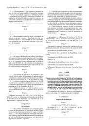
A <strong>first</strong>-<strong>use</strong> <strong>tutorial</strong> <strong>for</strong> <strong>the</strong> <strong>VIP</strong> <strong>Analysis</strong> <strong>software</strong><br />
Luis C. Dias<br />
INESC Coimbra & School of Economics - University of Coimbra<br />
Av Dias da Silva, 165, 3004-512 Coimbra, Portugal<br />
LMCDias@fe.uc.pt<br />
The <strong>software</strong> <strong>VIP</strong> <strong>Analysis</strong> supports decision-making in choice problems where a Decision Maker<br />
(DM) wishes to select an alternative from a set of several potential ones, accounting <strong>for</strong> multiple<br />
criteria at <strong>the</strong> same time. The underlying model is that of additive aggregation of value (or utility)<br />
functions, without needing to specify precise values <strong>for</strong> <strong>the</strong> model’s scaling constants that<br />
(indirectly) reflect <strong>the</strong> importance of each criterion. <strong>VIP</strong> <strong>Analysis</strong> implements a methodology to deal<br />
with Variable Interdependent Parameters presented in:<br />
Dias, L. C. & J. N. Clímaco, "Additive Aggregation with Variable Interdependent<br />
Parameters: <strong>the</strong> <strong>VIP</strong> <strong>Analysis</strong> Software", Journal of <strong>the</strong> Operational Research Society,<br />
Vol. 51, No. 9, pp. 1070-1082, 2000.<br />
This <strong>tutorial</strong> concerns <strong>the</strong> Version 1.0 of <strong>the</strong> <strong>software</strong>.<br />
INSTALLATION<br />
V.I.P. <strong>Analysis</strong> runs on Windows 95/98 computers, as well as posterior Microsoft operating systems.<br />
The monitor should be at least VGA (640x480) with 16 colors. It occupies very little space on disk<br />
and has minimum requirements in terms of RAM. The program may run without a mo<strong>use</strong>, but<br />
becomes somewhat cumbersome to <strong>use</strong>. You should have a 2-button mo<strong>use</strong> to make <strong>the</strong> best <strong>use</strong> of<br />
this <strong>software</strong>. To access <strong>the</strong> on-line manual you must have a default browser installed (e.g. Microsoft<br />
Explorer or Netscape).<br />
Unzip <strong>the</strong> file <strong>VIP</strong>1.zip to <strong>the</strong> folder where you want it to be located (e.g. <strong>the</strong> “Program Files”<br />
folder). The unzipped folder should contain <strong>the</strong> program (vip1.exe), a folder “Manual”, this<br />
document (vip_<strong>tutorial</strong>.pdf), and an example input file (example.vip). No updates to <strong>the</strong><br />
Windows registry or Start Menu are per<strong>for</strong>med. The <strong>software</strong> is now ready to run.<br />
1
GUIDED TOUR OF <strong>VIP</strong> ANALYSIS<br />
Start <strong>the</strong> program vip1.exe (e.g. double-click on its icon) and choose <strong>the</strong> option Open... from<br />
menu File (you may ei<strong>the</strong>r choose File|Open... or button ). Locate <strong>the</strong> file example.vip and<br />
press button OK (or press key ENTER).<br />
The initial data appear on <strong>the</strong> program window (Figure 1). For convenience, in any moment<br />
you may change <strong>the</strong> size of <strong>the</strong> window or maximize it, drag <strong>the</strong> splitter to <strong>the</strong> right or left,<br />
and/or change <strong>the</strong> size of <strong>the</strong> cells displaying <strong>the</strong> data (using <strong>the</strong> controls<br />
).<br />
Figure 1: Single-criteria value <strong>for</strong> 9 alternatives according to six value functions<br />
The data displayed on tab Data concern a situation analysed by Keeney and Nair in <strong>the</strong> 70s. We<br />
follow this study as reported by Roy and Bouyssou, who consider an additive aggregation model. 1<br />
This decision situation concerned <strong>the</strong> choice of a location <strong>for</strong> a nuclear plant, faced by <strong>the</strong><br />
Washington Public Power Supply System. There are nine potential sites (a 1 to a 9 ) and six criteria:<br />
impact on human health (crit1); loss of salmon (crit2); impact on o<strong>the</strong>r species (crit3); impact on<br />
economy (crit4); aes<strong>the</strong>tics (crit5); cost (crit6). The table on tab Data indicates <strong>the</strong> value of each<br />
alternative according to each of six criteria (v j (a i ), i=1,...,9, j=1,...,6). For instance, alternative a 1 is<br />
valued at 0.715 according to <strong>the</strong> <strong>first</strong> criterion (v 1 (a 1 )=0.715), being <strong>the</strong> worst alternative according<br />
that criterion (although it is <strong>the</strong> best one according to <strong>the</strong> fourth criterion, with v 4 (a 1 )=0.7316).<br />
According to <strong>the</strong> additive model, <strong>the</strong> overall value of each alternative is given by<br />
V(a i ) = k 1 v 1 (a i ) + k 2 v 2 (a i ) + ...+ k 6 v 6 (a i ),<br />
1 B. Roy and D. Bouyssou. Aide multicritère à la décision: méthodes et cas. Economica: Paris, 1993.<br />
2
where <strong>the</strong> parameters k 1 , ..., k 6 are denoted scaling constants and reflect <strong>the</strong> relative weight of <strong>the</strong> six<br />
value functions. More precisely, <strong>the</strong>y reflect trade-offs among <strong>the</strong> six value functions. These values<br />
are normalised such that k 1 + k 2 + ...+ k 6 = 1 and k 1 , ..., k 6 ≥ 0. The analysts started by asking some<br />
questions to <strong>the</strong> DMs and inferred from <strong>the</strong>ir answers <strong>the</strong> following order <strong>for</strong> <strong>the</strong> scaling constants:<br />
k 6 > k 1 > k 2 > k 4 > k 5 > k 3 .<br />
Then, <strong>the</strong>y continued asking questions to <strong>the</strong> DM to obtain precise values <strong>for</strong> <strong>the</strong>se parameters.<br />
The current status of <strong>the</strong> data reflect <strong>the</strong> intermediate stage where <strong>the</strong> analysts have inferred an<br />
order <strong>for</strong> <strong>the</strong> scaling constants, but have not yet tried to obtain more precise in<strong>for</strong>mation. The table<br />
on <strong>the</strong> Bounds tab (Figure 2) shows that no bounds <strong>for</strong> <strong>the</strong> parameters were fixed, apart from <strong>the</strong><br />
natural bounds that no scaling constant may be negative nor higher than 1.<br />
Figure 2: Lower and upper bounds <strong>for</strong> <strong>the</strong> scaling constants.<br />
Figure 3: Additional constraints <strong>for</strong> <strong>the</strong> scaling constants.<br />
The table that can be seen on <strong>the</strong> Constraints tab (Figure 3) shows <strong>the</strong> normalisation constraint (k 1 +<br />
k 2 + ...+ k 6 = 1) plus five additional constraints in five consecutive lines (from top to bottom: k 1 -<br />
k 6 ≤0, (-k 1 )+k 2 ≤0; (-k 2 )+k 4 ≤0; (-k 4 )+k 5 ≤0; and k 3 -k 5 ≤0;). Toge<strong>the</strong>r, <strong>the</strong>se five constraints define <strong>the</strong><br />
order k 6 ≥ k 1 ≥ k 2 ≥ k 4 ≥ k 5 ≥ k 3 .<br />
3
Hence, every possible combination of positive values <strong>for</strong> <strong>the</strong> scaling constants satisfying those<br />
constraints are considered equally acceptable <strong>for</strong> <strong>the</strong> moment. The role of <strong>VIP</strong> <strong>Analysis</strong> is now to<br />
discover which results (and conclusions) can be drawn considering this set of acceptable parameters.<br />
Figure 4: Summary of results.<br />
Figure 5: Range of value <strong>for</strong> <strong>the</strong> alternatives sorted by minimum value.<br />
As a <strong>first</strong> approach, <strong>VIP</strong> <strong>Analysis</strong> will compute <strong>the</strong> range of value <strong>for</strong> each alternative, i.e. <strong>the</strong><br />
minimum and maximum global value that each alternative may have, subject to <strong>the</strong> constraints on<br />
<strong>the</strong> scaling constants k 1 , ..., k 6 . Choose <strong>the</strong> option Range from <strong>the</strong> Results menu (Figure 3) to<br />
indicate this result is to be calculated and <strong>the</strong>n choose <strong>the</strong> option Calculate now! From <strong>the</strong> same<br />
menu. The right part of <strong>the</strong> <strong>VIP</strong> <strong>Analysis</strong> window will <strong>the</strong>n show <strong>the</strong> outputs (Figure 4 and Figure 5).<br />
Figure 4 indicates that alternatives a 5 and a 6 are absolutely dominated beca<strong>use</strong> <strong>the</strong>ir maximum value<br />
4
is less than <strong>the</strong> minimum value of a 1 . Hence, whatever <strong>the</strong> value <strong>for</strong> <strong>the</strong> scaling constants k 1 , ..., k 6 ,<br />
<strong>the</strong> alternatives a 5 and a 6 are considered worse than a 1 . The ranges may be seen graphically (Figure<br />
5) ei<strong>the</strong>r by input order (a 1 , a 2 , etc.) or by output order (sorted by <strong>the</strong>ir minimum value). The results<br />
show that a 2 and a 3 are <strong>the</strong> best according to <strong>the</strong> minimum value rule.<br />
The <strong>software</strong> offers <strong>the</strong> possibility of filtering <strong>the</strong> set of alternatives, based on <strong>the</strong>ir minimum<br />
value, maximum regret or on <strong>the</strong> possibility of being dominated. In this case, suppose <strong>the</strong> DM would<br />
pretend to focus on <strong>the</strong> alternatives with value always higher than 0.8. Choosing <strong>the</strong> option by Min<br />
Value of menu Filter allows to mark some alternatives as inactive (Figure 6). The inactive<br />
alternatives are not deleted, so that <strong>the</strong>y may be reactivated later. In this case, <strong>the</strong> marked<br />
alternatives are a 5 , a 6 , a 8 and a 9 , which appear with a red mark on <strong>the</strong> left part of <strong>the</strong> <strong>VIP</strong> <strong>Analysis</strong><br />
window, while <strong>the</strong>y are omitted from <strong>the</strong> results presented on <strong>the</strong> right part of <strong>the</strong> window (Figure 7)<br />
Figure 6: Filter.<br />
Figure 7: After filtering.<br />
Ano<strong>the</strong>r result that <strong>VIP</strong> <strong>Analysis</strong> can compute is <strong>the</strong> Pairwise Confrontation Table, which<br />
indicates <strong>the</strong> maximum advantage (difference of value) of each alternative over each o<strong>the</strong>r one. To<br />
per<strong>for</strong>m this, choose <strong>the</strong> Confrontation Table option from <strong>the</strong> Results menu and <strong>the</strong>n choose <strong>the</strong><br />
option Calculate now! from <strong>the</strong> same menu. The right part of <strong>the</strong> <strong>VIP</strong> <strong>Analysis</strong> window will <strong>the</strong>n<br />
show <strong>the</strong> table under tab Confrontation (Figure 8).<br />
Figure 8: Pairwise confrontation table.<br />
5
The negative cells are marked in red colour indicating that <strong>the</strong> alternative corresponding to <strong>the</strong><br />
respective row is dominated by <strong>the</strong> one corresponding to <strong>the</strong> respective column. Indeed, if <strong>the</strong><br />
maximum advantage (difference of value) is negative, <strong>the</strong>n this means that <strong>the</strong> row-alternative value<br />
is always lower than <strong>the</strong> column-alternative value <strong>for</strong> any values of k 1 , ..., k 6 respecting <strong>the</strong> imposed<br />
constraints. By considering only <strong>the</strong> constraints k 6 ≥ k 1 ≥ k 2 ≥ k 4 ≥ k 5 ≥ k 3 , it is possible to extract<br />
some interesting conclusions about a 2 and a 3 : <strong>the</strong>y are <strong>the</strong> only non-dominated ones and <strong>the</strong>y are <strong>the</strong><br />
best two in terms of minimum value and maximum regret. 2 These alternatives happened to be <strong>the</strong><br />
two with highest value in <strong>the</strong> original study.<br />
When <strong>the</strong> <strong>use</strong>r selects a cell, <strong>the</strong> program displays <strong>the</strong> value of <strong>the</strong> scaling constants that<br />
optimise it, as well as <strong>the</strong> inequalities that are binding at that optimum (<strong>the</strong>se are <strong>the</strong> constraints that<br />
might lead to a different optimum if <strong>the</strong>y were changed). For instance, <strong>for</strong> <strong>the</strong> selected cell (a 2 , a 3 ),<br />
<strong>the</strong> maximum advantage favourable to a 2 is 0.032, which occurs when k 6 = 1 and all o<strong>the</strong>r scaling<br />
constants are null. If <strong>the</strong> DM finds this unacceptable, <strong>the</strong>n he/she can add fur<strong>the</strong>r constraints. For<br />
instance, <strong>the</strong> DM may try to answer some questions regarding trade-offs among <strong>the</strong> criteria. Suppose<br />
that his/her answers imply <strong>the</strong> following constraints to add to <strong>the</strong> existing ones, using <strong>the</strong> option<br />
Insert from menu Constraints (Figure 9):<br />
• one unit of value in v 3 (.) is worth 0.06 units of value in v 2 (.) ⇒ -0.06 k 2 + k 3 = 0;<br />
• one unit of value in v 4 (.) is worth 0.26 units of value in v 6 (.) ⇒ k 4 - 0.26 k 6 = 0;<br />
• one unit of value in v 5 (.) is worth 0.15 units of value in v 6 (.) ⇒ k 5 - 0.15 k 6 = 0.<br />
Figure 9: New set of constraints.<br />
After confirming <strong>the</strong> changes (button Commit), <strong>the</strong> option Optimality from <strong>the</strong> Results menu<br />
becomes available, since <strong>the</strong> parameter space can now be illustrated in two dimensions. Choosing<br />
2 Maximum regret is <strong>the</strong> maximum disadvantage of an alternative when compared with any o<strong>the</strong>r alternative. It<br />
corresponds to <strong>the</strong> maximum value in each column, which is depicted graphically under tab Max regret (not<br />
illustrated here).<br />
6
that option and <strong>the</strong>n <strong>the</strong> option Calculate now! from <strong>the</strong> same menu produces new results. You can<br />
check that a 2 and a 3 are still <strong>the</strong> best in terms of minimum values (tab Ranges) and <strong>the</strong> ranges have<br />
become narrower, which is due to <strong>the</strong> fact that introducing constraints excludes some combinations<br />
of parameter values and corresponding results that were previously deemed acceptable. You can also<br />
check that a 2 and a 3 are <strong>the</strong> only non-dominated ones (tab Confrontation). A new tab Optimality<br />
appears with a graphical representation of <strong>the</strong> region in <strong>the</strong> parameter space where each alternative is<br />
<strong>the</strong> best. To observe figure 10 in your computer, per<strong>for</strong>m <strong>the</strong> following actions:<br />
• choose <strong>the</strong> tab Optimality;<br />
• select <strong>the</strong> row relative to a 3 and <strong>use</strong> <strong>the</strong> right button of <strong>the</strong> mo<strong>use</strong> to select <strong>the</strong> option Alternative<br />
at <strong>the</strong> bottom from <strong>the</strong> pop-up menu;<br />
• select <strong>the</strong> row relative to a 2 and <strong>use</strong> <strong>the</strong> right button of <strong>the</strong> mo<strong>use</strong> to select <strong>the</strong> option Alternative<br />
at <strong>the</strong> top from <strong>the</strong> pop-up menu;<br />
• resize <strong>the</strong> window, if needed;<br />
• click on a point in <strong>the</strong> green region;<br />
• drag <strong>the</strong> Tolerance “trackbar” a little to <strong>the</strong> right, so that <strong>the</strong> tolerance becomes 0.1.<br />
Figure 10: Optimality domains.<br />
Figure 10 displays <strong>the</strong> “optimality domains” of <strong>the</strong> two selected alternatives, showing where<br />
each of <strong>the</strong> two is <strong>the</strong> best among <strong>the</strong> set of alternatives. We can see that <strong>the</strong> two domains are not<br />
very different in size. The combination of values <strong>for</strong> <strong>the</strong> scaling constants that appears at <strong>the</strong> bottom<br />
7
(k 1 =0.204, k 2 =0.165, ...) corresponds to <strong>the</strong> point that was selected in <strong>the</strong> green region (you probably<br />
have selected a different one!). After that combination we can read <strong>the</strong> value of <strong>the</strong> two alternatives<br />
considering those parameter values (since we selected a point in <strong>the</strong> dark green region <strong>the</strong> value of a 2<br />
is higher than <strong>the</strong> value of a 3 (<strong>the</strong> reverse occurs in <strong>the</strong> dark blue region). Note that <strong>the</strong> dark grey<br />
region corresponds to parameter values that violate some constraint(s).<br />
The Tolerance control allows to tell <strong>the</strong> computer that a very small difference of value may be<br />
ignored. Setting <strong>the</strong> tolerance to 0.1, this means that a 2 is considered “quasi-optimal”, i.e. ei<strong>the</strong>r<br />
better than all <strong>the</strong> remaining ones, or worse but by a difference less than <strong>the</strong> tolerance. The light<br />
green domain shows that a 2 is quasi-optimal <strong>for</strong> all <strong>the</strong> acceptable parameter values, whereas a 3 is<br />
quasi-optimal in a domain representing 94.4% of <strong>the</strong> acceptable combinations of parameter values.<br />
Notice how <strong>the</strong> relation between <strong>the</strong> relative volumes is inverted when comparing a 2 with a 3 . You<br />
may also observe how <strong>the</strong> domains of quasi-optimality change as <strong>the</strong> tolerance decreases or<br />
increases. For all <strong>the</strong>se reasons, we believe that <strong>the</strong>se interactive graphical displays are a powerful<br />
tool of analysis and learning.<br />
CONCLUDING REMARK<br />
The choice between a 2 and a 3 is still open. Perhaps <strong>the</strong> DM has learned enough to make an<br />
in<strong>for</strong>med decision, or perhaps he/she is now capable of adding more constraints on <strong>the</strong> parameter<br />
values that will make a clear winner emerge. Or perhaps he/she has learned how to create a new<br />
alternative by combining <strong>the</strong> strengths of a 2 and a 3 . <strong>VIP</strong> <strong>Analysis</strong> intends to support <strong>the</strong> DM, and not<br />
to replace him/her. Whe<strong>the</strong>r you are na actual or prospective DM or analyst, or teacher or student, I<br />
hope you will find it valuable.<br />
8
![RL #35 [quadrimestral. Julho 2012] - Universidade de Coimbra](https://img.yumpu.com/27430063/1/190x234/rl-35-quadrimestral-julho-2012-universidade-de-coimbra.jpg?quality=85)