Salmon Chapter 4: Vorticity and turbulence

4
Vorticity and Turbulence
Turbulence is an immense and controversial subject. The next three chapters
present some ideas from turbulence theory that seem relevant to flow in the oceans and
atmosphere. In this chapter, we examine the connections between vorticity and
turbulence.
1. The vorticity equation
From ocean models that omit inertia, we turn to flows in which the inertia is a
dominating factor. Vorticity is of central importance, and, in the case of threedimensional
motion, we must take its vector character fully into account. We begin with
the equations
∂v
∂t + ( v ⋅ ∇)v
+ 2 Ω × v = − 1 ∇p − ∇Φ x
ρ ( )
p = p ρ,η
( )
∂ρ
∂t + ∇ ⋅( ρv)
= 0
(1.1)
∂η
∂t + ( v ⋅∇)η
= 0
for a perfect fluid in rotating coordinates. Here, Φ(x) is the potential for external forces,
η is the specific entropy, and the other symbols have their usual meanings. By the
general vector identity,
we have
where
∇( A⋅ B) = ( A ⋅∇)B + ( B ⋅∇)A + A × ( ∇ × B) + B × ( ∇ × A), (1.2)
∇( v ⋅ v) = 2( v ⋅ ∇)v + 2v × ω, (1.3)
ω ≡ ∇ × v (1.4)
is the vorticity. Thus, we can rewrite the momentum equation (1.1a) in the form
∂v
∂t + (ω + 2 Ω)×v = −∇P + p∇ ⎛ 1 ⎞
⎜ ⎟ , (1.5)
⎝ ρ⎠
IV-1

where
P ≡ p ρ + 1 2 v ⋅ v + Φ . (1.6)
Introducing the absolute velocity and vorticity,
v a ≡ v + Ω × r and ω a ≡ ∇ × v a = ω + 2Ω (1.7)
(respectively) in the nonrotating coordinate system, we can write (1.5) more compactly
as
∂v
∂t + ω ⎛
a × v = −∇P + p∇ 1 ⎞
⎜ ⎟ . (1.8)
⎝ ρ⎠
We form the vorticity equation by taking the curl of (1.8). By another general vector
identity,
we have
∇ × ( A × B) = A( ∇ ⋅B) − B( ∇⋅ A) + ( B ⋅∇)A − ( A ⋅ ∇)B, (1.9)
∇ × (ω a × v) = ω a (∇⋅ v) + 0 + (v⋅ ∇)ω a - (ω a ⋅∇)v, (1.10)
(since the divergence of a curl always vanishes). Thus the curl of (1.8) is
⎛ ∂
⎜
⎝ ∂t + v ⋅∇ ⎞
⎟ ω a + ω a (∇⋅v) = (ω a ⋅∇)v+ ∇p × ∇ 1 ⎠
ρ
(1.11)
Then, eliminating ∇⋅v between (1.11) and the continuity equation (1.1c), we finally
obtain
D
Dt (ω a/ρ) = [(ω a /ρ)⋅∇] v+ 1 ρ ∇p × ∇ 1 ρ
(1.12)
Eqn. (1.12) is the general vorticity equation for a perfect fluid. In the special case of
homentropic flow, in which the pressure depends only on the density, p=p(ρ), the last
term in (1.12) vanishes, and (1.12) reduces to
Dw
Dt
= ( w ⋅∇)v, (p = p( ρ)) , (1.13)
where
IV-2

w ≡ ω a /ρ (1.14)
is the ratio of the absolute vorticity to the density. 1 In the very special case of a constantdensity
fluid, (1.13) reduces to
Dω a /Dt = (ω a ⋅∇) v, (ρ=const.) (1.15)
2. Ertel’s theorem
According to the general vorticity equation (1.12), namely,
Dw
Dt
∇ρ × ∇p
= ( w ⋅∇)v + , (2.1)
ρ 3
the quotient w=ω a /ρ is conserved on fluid particles except for the terms on the righthand
side of (2.1). We shall see that the first of these terms, (w⋅∇)v, represents the tilting
and stretching of w. The last term in (2.1) represents pressure-torque. The pressuretorque
vanishes if the fluid is homentropic. We consider that case first.
If the fluid is homentropic, then (2.1) reduces to (1.13). To understand (1.13), let
δr( t) = r 2
( t) − r 1
( t) (2.2)
be the infinitesimal displacement between two moving fluid particles with position
vectors r 1 (t) and r 2 (t). Then
d
dt δr( t)
= d dt r ( t)
− d 2
dt r t 1
If δr is small, a Taylor-expansion of (2.3) yields
( ). (2.3)
d
dt δr i( t) = v i
( r 1
+ δr) − v i
( r 1
) = ∂v i
δr
∂x
j
, (2.4)
j
where the subscripts denote components, and repeated subscripts denote summation from
1 to 3. By comparing (2.4) to (1.13) in the form
Dw i
Dt
= ∂v i
∂x j
w j
, (2.5)
we see that the vector field w=ω a /ρ obeys the same equation as a field of infinitesimal
displacement vectors between fluid particles. We say that ω a /ρ is frozen into the fluid.
However, since the velocity field is continuous, the distortion experienced by ω a /ρ is
continuous. ω a /ρ can never be torn apart. Its topology is preserved despite distortion.
IV-3

These properties, so evident from the analogy between ω a /ρ and δr, lie at the heart of the
many vorticity theorems in fluid mechanics.
The most important of these is Ertel’s theorem. Still considering the case of
homentropic flow, let θ(x,t) be any scalar conserved on fluid particles,
Dθ
Dt = 0 . (2.6)
The scalar θ need not have physical significance; it could be an arbitrarily defined
passive tracer. Let r 1 (t) and r 2 (t) be defined as before. Then (2.6) implies that
d
dt θ r 1( t),t
( ) − d dt θ ( r 2( t),t) = 0 . (2.7)
If the distance between the two fluid particles is infinitesimal, then (2.7) becomes
Now let
d
dt
δr i
0
⎡ ∂θ ⎤
⎢ δr
∂x
j ⎥ = 0. (2.8)
⎣ j ⎦
( ) = γ w i
r 1
0
( ( ),0) (2.9)
where w(r 1 ,0) is the initial w at the location r 1 , and γ is an infinitesimal constant with
appropriate dimensions. In other words, choose the two fluid particles to lie
infinitesimally far apart along a line parallel to the vorticity. Then, since w and δr obey
the same equation,
δr i
( t) = γ w i
( r 1
,t) (2.10)
at later times t. Since γ is a constant, it follows from (2.8) and (2.10) that
D
Dt
⎡ ∂θ ⎤
⎢ w
∂x
j ⎥ =
⎣ j ⎦
D [
Dt ∇θ ⋅ w ] = 0 (homentropic flow). (2.11)
Eqn. (2.11) is Ertel’s theorem for homentropic fluid. According to (2.11),
homentropic flow conserves ∇θ⋅ω a /ρ on fluid particles, where θ is any conserved scalar
satisfying (2.6). This derivation shows that (2.11) rests on nothing besides the frozen-in
nature of the field ω a /ρ.
In the general case of non-homentropic flow, (2.11) generalizes easily to
∇θ ⋅ ∇ρ × ∇p
[ ] = ( )
D
∇θ ⋅w
Dt
ρ 3 (2.12)
IV-4

and ∇θ⋅w is not conserved on fluid particles. The right-hand side of (2.12) arises from
the pressure-torque in (2.1). However, if we choose the scalar θ to be (any function of)
the entropy η (which satisfies (2.6)), then the right-hand side of (2.12) vanishes (because
p=p(ρ,η)), and (2.12) reduces to
where
DQ
Dt
= 0, (2.13)
Q ≡ (ω a ⋅ ∇η) / ρ (2.14)
is the potential vorticity. Eqn. (2.13), also called Ertel’s theorem, is the most general
statement of potential vorticity conservation. The potential vorticity laws obtained in
previous chapters (from various approximations to (2.1)) can all be be viewed as
approximations to (2.13-14).
Of course, we can prove all these results directly from (1.1) by pedestrian
mathematical manipulations, but that makes it harder to appreciate their physical
significance.
3. A deeper look at potential vorticity
Again assume that the fluid is homentropic. Let θ 1 (x,t), θ 2 (x,t), and θ 3 (x,t) be any
three independent (but otherwise arbitrary) scalars satisfying
Dθ 1
Dt
= 0,
Dθ 2
Dt
= 0,
Dθ 3
Dt
= 0 . (3.1)
By independent we mean that ∇θ 1 , ∇θ 2 , and ∇θ 3 everywhere point in different
directions. It is easy to see that if the θ i are initially independent, then they remain so by
(3.1). (One possible choice for the θ i would be the initial Cartesian components of the
fluid particles.) Since the fluid is homentropic, Ertel’s theorem (2.11) tells us that
DQ 1
Dt
= 0,
DQ 2
Dt
= 0,
DQ 3
Dt
= 0 , (3.2)
where
Q 1
= w ⋅ ∇θ 1
, Q 2
= w⋅ ∇θ 2
, Q 3
= w⋅ ∇θ 3
(3.3)
are the potential vorticities corresponding to the θ i .
Since the θ i are independent, we can regard them as curvilinear coordinates in xyzspace.
By (3.1), these curvilinear coordinates are also Lagrangian coordinates, because
IV-5

the surfaces of constant θ i move with the fluid. We regard the vectors ∇θ 1 , ∇θ 2 , and ∇θ 3
as basis vectors attached to the Lagrangian coordinates. As the fluid moves, these basis
vectors tilt and stretch with the flow. By (3.3), the conserved Q i are just the dot-products
(3.3) of w with these moving basis vectors. The dot-products are conserved because the
tilting and stretching terms on the right-hand side of (1.13), which destroy the
conservation of w, are taken into account by the motion of the basis vectors ∇θ i . 2
Now let A=(A 1 , A 2 ,A 3 ) be the components of the (absolute) velocity v a with respect to
these same basis vectors. That is, let
v a
= A 1
∇θ 1
+ A 2
∇θ 2
+ A 3
∇θ 3
. (3.4)
We shall show that, with a very weak further restriction on the choice of θ i ,
where
Q ≡ ( Q 1
,Q 2
,Q 3
) = ∇ θ
× A , (3.5)
⎛ ∂ ∂ ∂ ⎞
∇ θ
≡ ⎜ , , ⎟ (3.6)
⎝ ∂θ 1
∂θ 2
∂θ 3 ⎠
is the gradient operator in the Lagrangian coordinates. That is, the conserved potential
vorticity Q is the curl of the absolute velocity v a in Lagrangian coordinates. Then Ertel’s
theorem (3.2) can be written in the suggestive form
D
Dt ∇ × A θ
( ) = 0. (3.7)
Hence, the potential vorticity (3.5) is just ordinary vorticity measured in Lagrangian
coordinates. If the fluid is homentropic, then (3.7) implies that the potential vorticity is
simply a static vector field,
∇ θ
× A = F( θ 1
,θ 2
,θ 3
) , (3.8)
in θ 1, θ 2 ,θ 3 -space, where F is determined by the initial conditions. A translation of (3.8)
into conventional notation yields what some writers call Cauchy’s solution of the vorticity
equation.
To show that (3.5) agrees with (3.3), we suppress the subscript a on ω a and v a , and
compute
Q r = (ω⋅∇θ r )/ρ =
Thus
1 ρ ε ijk
∂v k
∂x j
∂θ r
∂x i
= 1 ρ ε ijk
∂
∂x j
⎛ ∂θ
A s
⎞
⎜ s ⎟ ∂θ r
= 1
⎝ ∂x k ⎠ ∂x i
ρ ε ijk
∂θ r
∂x i
∂A s
∂x j
∂θ s
∂x k
. (3.9)
IV-6

( )
∂( x, y,z )
Q r
= 1 ∂ θ r
, A s
,θ s
ρ
( )
∂( x, y,z)
= 1 ∂ θ 1
,θ 2
,θ 3
ρ
( )
∂( x,y, z)
= 1 ∂ θ 1
,θ 2
,θ 3
ρ
ε ijk
∂θ r
∂θ i
∂A s
∂θ j
∂θ s
∂θ k
( )
( )
( )
∂( x,y, z)
∂ θ r
, A s
,θ s
∂ θ 1
,θ 2
,θ 3
= 1 ∂ θ 1
,θ 2
,θ 3
ρ
ε rjs
∂A s
∂θ j
(3.10)
That is,
( )
∂( x,y, z)
Q r
= 1 ∂ θ 1
,θ 2
,θ 3
ρ
[ ∇ θ
× A] r
. (3.11)
If the Lagrangian coordinates are mass-labeling coordinates in the sense of Chapter 1,
that is, if
dθ 1
dθ 2
dθ 3
= d( mass), (3.12)
then (3.11) reduces to (3.5). (In Chapter 1 we used the symbols a,b,c to denote masslabelling
coordinates, and ∂/∂τ to denote D/Dt.)
In general non-homentropic flow, the pressure-torque on the right-hand side of (2.1)
destroys two of the three components of the conservation law (3.7). In that case, it is
convenient to take the entropy η as one of the Lagrangian coordinates. Then, since the
pressure-torque in (2.1) has no component in the direction of ∇η, the η-component of
(3.7) survives,
D
Dt (∇ θ × A) ⋅∇ θη
[ ] = 0 . (3.13)
By steps similar to those in (3.9) and (3.10), we can show that the conserved quantity in
(3.13) is the general potential vorticity (2.14).
Although (3.13) contains only one-third of the dynamical information in (3.7), it is —
in strongly stratified flow — a much more useful equation. In unstratified (∇η=0) flow,
the θ i -surfaces typically become very convoluted, and the simplicity of the Lagrangian
equation (3.7) is offset by the complexity of transforming this result back into xyzcoordinates.
However, in strongly stratified flow, the gravitational restoring forces resist
the folding of isentropic surfaces, rendering the single equation (3.13) much more useful.
Moreover, if the fluid is rapidly rotating, then (3.13) controls the nearly geostrophic part
of the motion (as we have seen in Chapter 2).
4. Alternative statements of the vorticity law
As we have seen, the quotient ω a /ρ is conserved on fluid particles except for the
effects of tilting, stretching and pressure-torque. However, the effects of tilting and
stretching can be absorbed into a Lagrangian description of the motion. Then only
IV-7

pressure-torque stands in the way of conservation. In this section, we examine alternative
(and more conventional) ways of saying these same things.
First, consider the circulation
C ≡
∫ v ⋅ dr , (4.1)
where the integration is around a closed material loop of fluid particles, that is, around a
loop that always contains the same fluid particles. By Stokes’s theorem
C = ∫∫
ω ⋅n dA , (4.2)
where n is the normal to an arbitrary surface containing the loop. If the fluid is rotating,
we also define the circulation relative to the inertial reference frame,
C a
≡
∫ v a
⋅ dr = ∫∫ (ω + 2Ω)⋅n dA . (4.3)
Now, by the momentum equation (1.1a) for a rotating fluid,
dC a
dt
=
=
=
∫
∫
∫
D
Dt
[( v + Ω × r) ⋅ dr]
⎡ ⎛ Dv
⎜
⎝ Dt + Ω × v ⎞
⎤
⎟ ⋅ dr + ( v + Ω × r)⋅ dv
⎣ ⎢
⎠
⎦ ⎥
⎛ Dv
⎜
⎝ Dt + 2Ω × v ⎞
⎟ ⋅ dr
⎠
⎛
= − 1 ⎞
∫ ⎜ ∇p − ∇Φ⎟ ⋅ dr
⎝ ρ ⎠
= −∫
dp
ρ
(4.4)
If the fluid is homentropic, then p=p(ρ) and the right-hand side of (4.4) vanishes; the
circulation (4.3) is conserved.
We see that the effects of vortex tilting and stretching are built in to the definition of
circulation. The material loop of fluid particles tilts and stretches with the motion of the
fluid. Only the pressure-torque, represented by the last term in (4.4), causes the
circulation to change. And, as anticipated by our discussion of Ertel’s theorem, even the
pressure-torque does not entirely destroy the conservation of circulation; the circulation
is conserved if we choose the material loop of fluid particles to lie entirely within a
surface of constant entropy.
The concept of vortex tubes offers another way to describe the frozen-in evolution of
the vorticity field. Suppose that the fluid is nonrotating. (The extension to rotating
coordinates is easy.) At a fixed time t, choose an arbitrary closed loop within the fluid,
and consider the tube formed by its indefinite extension in the direction of the vorticity
IV-8

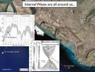
ω. Refer to Figure 4.1. At the same fixed time, consider two loops, L 1 and L 2 , around
the vortex tube. Since ω is everywhere tangent to the sides of the vortex tube, and
∇⋅ω=0, (4.5)
the divergence theorem tells us that
∫∫ ω ⋅ n 1 dA 1 = ∫∫ ω ⋅ n 2 dA 2 , (4.6)
where n i are the unit normals to surfaces containing the loops L i , and dA i are the
corresponding area elements. Thus, the strength of the vortex tube is the same at every
cross-section.
Now suppose that the fluid is homentropic. Then the vortex tube is a material
volume that moves with the fluid particles composing it; by the analogy between ω/ρ
and the infinitesimal displacement vector between fluid particles on the surface of the
vortex tube, ω remains tangent to the moving surface of the vortex tube. Hence the
strength of the vortex tube remains uniform along the tube. Moreover, the circulation
theorem tells us that
d
dt
∫∫ ω ⋅ n dA = 0, (4.7)
so that the strength of the vortex tube is also constant in time. The vortex tube can
stretch, increasing its vorticity, but the cross-sectional area then experiences a
compensating decrease. Once again, the effects of tilting and stretching have been built
into a definition in order to produce a conservation law.
We can think of any homentropic flow as a (generally complicated) tangle of vortex
tubes. (Think of a big pile of spaghetti, with each noodle a closed loop.) As the flow
evolves, these vortex tubes experience a continuous distortion, but (in the absence of
friction) their strength and their topology are obviously preserved.
Helicity is a vorticity invariant that reflects the topology. Let V be a closed material
volume of homentropic fluid whose surface is (and remains) everywhere tangent to the
vorticity ω. That is, let V be a collection of closed vortex tubes. Then the helicity,
H t
is conserved,
∫∫∫ ω dV (4.8)
( ) ≡ v ⋅
V
dH
dt
= 0 . (4.9)
This follows from
IV-9

DH
Dt
=
=
=
=
∫∫∫
V
V
∫∫∫
= D Dt
V
D
Dt
v ⋅ (ω/ρ) ρ dV
[ v ⋅ (ω/ρ) ] ρ dV
∫∫∫ [ D Dt v ⋅ (ω/ρ) + v ⋅ D Dt
∫∫∫
V
V
[ - ∇P⋅ ω + v ⋅ (ω ⋅ ∇) v ] dV
∫∫∫ [ - ∇⋅ (Pω) + 1 2 ∇⋅ ( ω v⋅v) ] dV = 0,
(ω/ρ)] ρ dV (4.10)
where dP=dp/ρ +dΦ. The last line vanishes because ω is tangent to the surface of V.
The helicity H turns out to be a measure of the knotted-ness of the material volume of
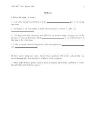
vortex tubes. 3 Consider, for example, two thin vortex tubes (represented abstractly as
lines) with volumes V 1 and V 2 , that are linked together as shown in Figure 4.2. The
vortex lines within each tube are simple, parallel (i.e. untwisted) closed curves. The
arrows point along the tubes in the direction of the vorticity, n i are unit normals to
surfaces S i containing the axes of the tubes, and the vorticity outside the tubes is assumed
to vanish. By definition,
But
H = ∫∫∫ v ⋅ ω dV 1+ ∫∫∫ v ⋅ ω dV 2. (4.11)
∫∫∫ v ⋅ ω dV 1 = ∫ dr 1 ∫∫ dA 1
= dr 1
v ⋅∫∫
dA 1
where ω=|ω| and
v ⋅ ω
∫ ω = ∫ dr 1
⋅ v∫∫
dA 1
ω = κ 1 ∫ dr 1
⋅ v
(4.12)
κ 1
≡ ∫∫ ω dA 1
(4.13)
is the (constant) strength of vortex tube 1. On the other hand,
∫ dr 1
⋅ v = ∫∫ ω ⋅ n 1 dS 1 = κ 2 , (4.14)
where κ 2 is the strength of vortex tube 2. Thus, (4.12) becomes
∫∫∫ v ⋅ω dV 1 = κ 1 κ 2. (4.15)
By similar steps,
IV-10

∫∫∫ v ⋅ω dV 2 = κ 2 κ 1 . (4.16)
Hence the helicity (4.11) is
H = 2κ 1
κ 2
. (4.17)
If the vortex tubes were not linked, we would find that H=0. If the vorticity in one of the
tubes were reversed, then H would change sign. If both tubes were reversed, then H
would be unchanged, but the resulting configuration is simply a rotated version of the
sketch in Figure 4.2.
Again we emphasize that all these vorticity laws are direct consequences of the
frozen-in nature of vorticity in the case of homentropic flow. Ertel’s theorem, which
amounts to a transformation of the vorticity equation into Lagrangian coordinates, is the
most illuminating of these vorticity laws, but helicity conservation is perhaps the most
exotic. However, helicity conservation applies only to material volumes of closed vortex
tubes, and thus excludes those portions of the fluid whose vortex tubes terminate at
boundaries. Moreover, although there is a helicity invariant corresponding to every
subvolume of closed vortex tubes, it is easy to imagine a very complicated vorticity
distribution in which a single vortex line passes arbitrarily close to every point in the
fluid. Then the only subdomain of closed vortex tubes is the whole fluid, and (because
vortex tube linkages with opposite signs produce cancelling contributions to the helicity)
the single helicity invariant cannot tell us very much about the topology of the vorticity
field.
5. Turbulence
Every aspect of turbulence is controversial. Even the definition of fluid turbulence is
a subject of disagreement. However, nearly everyone would agree with some elements of
the following description:
(1.) Turbulence is associated with vorticity. In any case, the existence of vorticity is
surely a prerequisite for turbulence in the sense that irrotational flow is smooth and
steady to the extent that the boundary conditions permit. 4
(2.) Turbulent flow has a very complex structure, involving a broad range of spaceand
time-scales.
(3.) Turbulent flow fields exhibit a high degree of apparent randomness and disorder.
However, close inspection often reveals the presence of orderly embedded flow structures
(sometimes called coherent structures).
(4.) Turbulent flows are three-dimensional (unless constrained to be two-dimensional
by strong rotation or stratification), and have a high rate of viscous energy dissipation.
(5.) Advected tracers are rapidly mixed by turbulent flow.
(6.) Turbulent flow fields often exhibit high levels of intermittency. (Roughly
speaking, a flow is intermittent if its variability is dominated by infrequent large events.)
However, one further property of turbulence seems to be more fundamental than all of
these others, because it largely explains why turbulence demands a statistical treatment.
IV-11

This property has been variously called instability, unpredictability, or lack of bounded
sensitivity. In more fashionable terms, turbulence is chaotic.
To understand what this means, consider two turbulent flows, both obeying the
Navier-Stokes equations (say), but beginning from slightly different initial conditions.
Experience shows that no matter how small the initial difference, the two flows will
rapidly diverge, and will soon be as different from each other as if the initial difference
had been 100%.
This instability property has practical consequences. Imagine a laboratory
experiment with a turbulent fluid, in which the experimenter measures some arbitrary
flow quantity V(t) as a function of time. For example, V(t) could be the temperature or
velocity at a fixed point in the flow. Refer to Figure 4.3. The experimenter is interested
in V(t 1 ), the value at time t 1 . To be sure of his result, he repeats the experiment,
arranging the apparatus and initial conditions to be as nearly the same as possible. But no
matter how hard he tries, the new value of V(t 1 ) is always discouragingly different from
the original measurement. The experimenter is finally satisfied to repeat the experiment a
great many times, and to compute the probability distribution of V(t 1 ). He becomes a
statistician. Because of the instability property, he reasons, only statistics are of value in
predicting the outcome of future experiments.
The question arises: Can the statistics be found without actually performing all of the
experiments? That is, can the statistical averages of turbulent flow be calculated from
physical law, without first solving the equations (either experimentally or with a big
computer) and then averaging the results of many solutions? Many people regard this
unanswered question as the central problem of turbulence.
The most direct approach to the prediction of statistics is to average the equations of
motion, thereby obtaining evolution equations for the averages. Unfortunately, as
explained in Chapter 1, direct averaging leads to an unclosed hierarchy of statistical
moment equations, in which the equation for the time derivative of the n-th moment
always involves the (n+1)-th moment. These moment equations cannot be solved
without making additional hypotheses to close them. We set aside this closure problem
until Chapter 5, and thus temporarily abandon any hope of obtaining a complete
statistical description of turbulent flow. However, we find that many of the important
qualitative properties of turbulence can perhaps be understood on the basis of relatively
simple ideas, many of which involve vorticity.
6. Kolmogorov’s Theory
Now we consider constant-density flow governed by the Navier-Stokes equations,
∂v i
∂t
∂v i
∂x i
= 0
+ v j
∂v i
∂x j
= − ∂p
∂x i
+ν ∂ 2 v i
∂x j
∂x j
(6.1)
IV-12

Once again, the summation convention applies to repeated subscripts. First we review
elementary properties of (6.1). Then we examine the most famous (but still very
controversial!) theory of three-dimensional turbulence.
In principle, it is always possible to rewrite (6.1) as a single, prognostic equation in
the velocity v=(v 1 ,v 2 ,v 3 ). This converts the pressure term in (6.1a) into a nonlinear term
like the advection term. To see this, we take the divergence of (6.1a) to obtain an elliptic
equation,
∂v j
∂x i
∂v i
∂x j
= − ∂ 2 p
∂x i
∂x i
= −∇ 2 p , (6.2)
for the pressure p. Given the velocity field v(x) and the appropriate boundary condition,
we can solve (6.2) for p(x). For fluid inside a rigid container, the appropriate boundary
condition is v=0. The boundary condition v=0 implies that
0 = − ∂p
∂x n
+ ν ∂ 2 v n
∂x n
2
(no summation on n) (6.3)
on the boundary, where n denotes the direction normal to the boundary. Eqn. (6.2) and
the Neumann boundary condition (6.3) determine the pressure throughout the flow. Only
in simple geometry (like that considered below) is it possible to solve (6.2-3) explicitly,
but (at least in principle) it is clearly always possible to replace the pressure term in
(6.1a) by a quadratic expression in the velocity.
Next we consider the energy equation obtained by contracting the momentum
equation (6.1a) with v i , namely
∂
∂t
1
( 2 v i
v i
) + ∂
∂x j
1
( 2 v i
v i
v j ) = − ∂
∂x i
∂
( v i
p) 2 v
+ νv i
i
. (6.4)
∂x j
∂x j
Integrating (6.4) over the whole domain inside the rigid boundary, and using the
boundary condition v=0, we obtain
d
dt
⎡
dx 1 2
v i
v i
= ν dx ∂ ⎛ ∂v ⎞
⎜ v i
i
⎟ − ∂v i
∂v
⎤
∫∫∫
⎢
i
⎥
⎣ ⎢ ∂x j ⎝ ∂x j ⎠ ∂x j
∂x j ⎦ ⎥
∫∫∫ = −ν dx ∂v i
⎢
⎡ ∂v ⎤
∫∫∫
i
⎥ . (6.5)
⎣ ∂x j
∂x j ⎦
Thus, neither the advection term nor the pressure term affects the total energy, but the
viscous term always causes energy to decrease.
If the flow is spatially unbounded, then it is illuminating to examine the Fourier
transforms of these equations. Let
v i
( x,t) = ∫∫∫ dk u i
( k,t)e ik⋅x
. (6.6)
Since v(x,t) is real, its Fourier transform u(k,t) is conjugate symmetric,
IV-13

u i
( k) = u i
( −k) *. (6.7)
By Fourier’s theorem,
u i
( k,t) =
Similarly, let
1
dx v
( 2π ) 3 i
x,t
∫∫∫ ( )e −ik⋅x
. (6.8)
p( x,t) = ∫∫∫ dk p( k,t)e ik⋅x . (6.9)
Then the elliptic equation (6.2) for the pressure becomes
∫∫∫ ∫∫∫
( ) e i( m⋅x +n⋅x)
= − dm −m 2
− dm dn m i
u j
( m)n j
u i
n
im ⋅x
∫∫∫ ( )p( m)e (6.10)
where m=|m|, etc. Multiplying (6.10) by e -i k⋅x and integrating over all x, we obtain the
Fourier tranform of (6.2) in the form
−∫∫∫ dm∫∫∫
dn m i
n j
u j
( m)u ( i
n )δ( m + n − k)
= k 2 p( k)
. (6.11)
Then, using (6.11), and proceeding in a similar manner, we obtain the Fourier transform
of the momentum equation (6.1a) in the form
∂
∂t u i( k,t) + i∫∫∫
dm∫∫∫
dn n j
u j
( m)u i
( n)δ( m + n − k)
∫∫∫
∫∫∫
= i dm dn k i m r n j
k 2
u j
( m)u r
( n)δ( m + n − k) − νk 2 u i
( k)
(6.12)
More concisely,
∂
∂t u i( k,t) = ∫∫∫ dm∫∫∫
dn A ijr
( m,n,k) u ( j
m )u ( n)δ(
m + n − k)
−νk 2 u ( k)
, (6.13)
r i
where A ijr (m,n,k) is the coupling coefficient between u i (k), u j (m), and u r (n). The
nonlinear term on the left-hand side of (6.12) represents the advection of momentum.
The nonlinear term on the right-hand side of (6.12) represents the effect of pressure.
Thus the A ijr -term in (6.13) represents both pressure and advection.
If pressure and advection were absent, (6.13) would be a linear equation,
∂
∂t u i( k,t) = −νk 2 u i
( k), (6.14)
IV-14

in which the various wavenumbers are uncoupled. The solution of (6.14) is
u i
( k,t) = u i
( k,0) exp( −νk 2 t) . (6.15)
According to (6.15), the velocity in wavenumber k decays exponentially, at a rate that
increases with increasing wavenumber magnitude k. Thus, viscosity damps the smallest
spatial scales fastest.
The nonlinear terms in (6.13) are much more complicated than the viscous-decay
term and take the form of triad interactions that couple together wavenumbers satisfying
the selection rule m+n=k. As we already know, these triad interactions do not change
the total energy,
∫∫∫ dx
∞
1
2 v i
v i
= 4π 3 ∫∫∫ dk u i
( k)u i
( k)* ≡ ∫ dk E( k)
⋅∫∫∫
dx , (6.16)
0
but they do transfer energy between wavenumbers satisfying the selection rule. 5 The last
equality in (6.16) defines the energy spectrum E(k).
Now consider the following situation: an initially quiescent fluid, in a container of
size L, is stirred by some external agency at lengthscales comparable to L. Suppose that
this stirring force is nonzero only for L -1

ightward (that is, toward higher k) through the spectrum. The latter rate is equal to ε, the
rate of energy dissipation per unit volume. Refer to Figure 4.5. On the inertial range
between K F and K D , the wavenumber at which viscous dissipation first becomes
important, the spectrum E(k) should depend only on ε and k. The dimensions of these
quantities are
[ E( k)
] = L 3 T −2 , [ ε] = L 2 T −3 , [ k] = L −1 , [ ν] = L 2 T −1 . (6.17)
Hence, dimensional analysis tells us that
E( k) = Cε 2 / 3 k −5/ 3 and K D
= O( ε 1/ 4 ν −3/ 4
), (6.18)
where C is Kolmogorov’s universal constant.
Observed spectra often agree with (6.18a) and suggest that C≈1.5. Nevertheless,
considerable uncertainty surrounds this whole subject. It is now generally agreed that
Kolmogorov’s theory cannot in principle be exactly right, and experimental
measurements of higher statistical moments, which are also predicted by the complete
Kolmogorov theory, do not support the theory. We consider these points in the next
section.
7. Intermittency and the beta-model
In a famous footnote to his book on fluid mechanics, L. D. Landau noted an important
inconsistency in K41. This led to a revision of the theory, but most people feel that it
also destroyed any hope that the theory can be exactly right. 7 Landau’s objection is
neither the only, nor perhaps even the most serious objection to K41. However, it has
helped theorists to better appreciate the enormous assumptions underlying Kolmogorov’s
theory.
The essence of Landau’s objection is that K41 cannot apply to a collection of flows
with different dissipation rates ε. First consider two completely separate flows, denoted
by the subscripts 1 and 2. The first flow is vigorously stirred, so that ε 1 is large. The
second flow is only moderately stirred, so that ε 2 is small. If both flows are turbulent,
then according to K41,
E 1
2 /
( k) = Cε 3 1
k −5 / 3 and E 2
k
( ) = Cε 2
2 / 3 k −5/ 3 . (7.1)
Next, consider the composite system consisting of these two separate flows. If the
two flows have equal volumes, then the dissipation rate and the energy spectrum of the
composite system are given by
But then
ε = 1 2 ( ε 1
+ ε 2
) and E k
( ) = 1 2 ( E 1
( k) + E 2
( k)
). (7.2)
IV-16

E( k) ≠ Cε 2 / 3 k −5/ 3 . (7.3)
That is, the composite system cannot obey K41, essentially because the average of a twothirds
power is not the power of the average.
So far there is no problem, because the composite flow is not a single flow, and hence
there is no reason why K41 should apply to it. But suppose that the subscripts 1 and 2
refer not to separate flows, but to large regions of the same flow with locally different
dissipation rates. We conclude uncomfortably that K41 cannot apply to the whole flow if
it is also locally correct. In particular, K41 should fail in cases where the dissipation rate
ε averaged over length-scales characteristic of the inertial range fluctuates.
The beta-model is a schematic model that clarifies this argument and suggests the
nature of the correction to K41. 8 Consider a turbulent flow in a container of size L 0 . The
fluid is stirred on scales comparable to L 0 , and the energy is subsequently transferred to
smaller spatial scales via the nonlinear terms in the momentum equations. Again we
suppose this transfer to be a series of cascade steps from scale L 0 to L 1 =L 0 /2 to L 2 =L 1 /2,
and so on. (The factor of 1/2 is inessential; any other fraction will work.) The n-th
cascade step corresponds to eddy-size
We also define:
L n
= L 0
2 ≡ k −1 n n
. (7.4)
V n , the characteristic velocity change across eddies of size L n
ε n , the rate at which energy passes through the n-th cascade step; and
E n
=
k n+ 1
∫ E( k )dk .
k n
E n is the energy (per unit volume of the whole flow) contained in eddies of size L n .
Now, the cascade can proceed in two ways, as shown in Figure 4.6. At each cascade
step, the eddies created can fill the whole space uniformly, or they can fill only a fraction
β of the available space and be correspondingly stronger. We shall see that the K41
theory corresponds to the first alternative (β =1).
For general β, the total energy in eddies of size L n is the energy within the eddies
themselves, V n 2 , times the fraction β n of the total volume occupied by these eddies. That
is,
E n
~ β n V n 2 , (7.5)
where the symbol ~ denotes very rough equality. This energy moves through the n-th
cascade step in a turn-over time
IV-17

T n
~ L n
V n
= 1
k n
V n
, (7.6)
so that
ε n
~ E n
T n
~ β n V n 3 k n
. (7.7)
If the turbulence is stationary, then ε n must be independent of n; otherwise the energy
would pile up at some intermediate wavenumber. But if
ε n
= ε , (7.8)
then (7.5) and (7.7) imply that
Since
E n
~ ε 2 / 3 k n
−2 / 3 β n / 3 . (7.9)
E n
=
k n+ 1
∫ E( k )dk = ∫ kE( k)d( ln k)
k n
ln k n+1
ln k n
∝ k n
E( k n
), (7.10)
(7.9) corresponds to the spectrum
E( k n
) ~ ε 2 / 3 −5 /
k 3 n
β n / 3 . (7.11)
According to (7.11), the energy spectrum at wavenumber k n is smaller than that
predicted in K41 by the factor β n/3 (where β0) turbulence, the spectrum falls off more steeply. Physically, the
IV-18

steeper fall-off occurs because spatial concentration of the eddies makes them more
intense, and thus shortens the residence time (7.6) for energy at each cascade step.
Observations support the prediction of K41 (with s =0) for the spectrum, 9 but suggest
increasing disagreement with K41 as higher-order moments are considered. 10 Recall that
the spectrum is the Fourier transform (with respect to r) of
F( r) ≡ v i
( x + r)v i
( x) , (7.15)
where we assume that the flow is statistically homogeneous and isotropic. As an
example of a higher-order statistic, consider the structure function
F p
( r) ≡ v x + r
( ) − v( x) p . (7.16)
If r -1 lies within the inertial range, then, by dimensional analysis, K41 predicts that
v( x + r) − v( x) p = C p
( ε r) p/ 3 , (7.17)
where C p is a universal constant. On the other hand,
G p
( r) ≡ v( x + r) − v( x) 2 p / 2 = D p
ε r
( ) p / 3 , (7.18)
where D p is another universal constant. Thus, because (7.17) and (7.18) have the same
dimensions, their ratio
R p
≡ F p
( r)
r
G p
( ) = v( x + r) − v( x) p
v( x + r) − v( x) 2 p / 2 = C p
D p
(7.19)
must be a universal constant, independent of ε and r. When p=4, the quantity (7.19) is
called kurtosis.
Observations suggest that (7.19) increases with p and with r -1 . Since R p measures
spatial intermittency (more sensitively for larger p), these observations suggest a spatial
intermittency that increases with decreasing eddy size. This contradicts K41, and it
suggests that the eddies of decreasing size are indeed confined to a decreasing fraction of
the fluid volume, as in the beta-model.
The beta-model predicts that
and
⎛ 1 ⎞
F p ⎜ ⎟ ~ β n V n
⎝ ⎠
k n
( ) p (7.20)
IV-19

⎛ 1 ⎞
G p ⎜ ⎟ ~ β n 2
V n
⎝ ⎠
k n
( ) p / 2 . (7.21)
Hence the beta-model prediction for (7.19) is
That is,
⎛
R p
~ β n(1− p / 2 ) ~ ⎜
⎝
k n
k 0
⎞
⎟
⎠
− s+ sp/ 2
. (7.22)
R p
⎛
( r) ~ r ⎞
⎜ ⎟
⎝ L 0 ⎠
s− sp/ 2
. (7.23)
If the cascade is space-filling (s=0), then (7.23) is independent of r, in agreement with
K41. However, for s>0 and p >2, R p (r) increases with decreasing r.
8. Two-dimensional turbulence
Again we consider constant-density flow governed by the Navier-Stokes equations.
Now, however, we suppose that the flow is two-dimensional,
v = ( u( x, y),v( x,y), 0), (8.1)
so that the vorticity equation,
reduces to
Here,
D
Dt ω = (ω ⋅ ∇) v + ν ∇2 ω, (8.2)
Dω
Dt
= ν∇ 2 ω . (8.3)
⎛
ω = ω k =
∂v
∂x − ∂u ⎞
⎜ ⎟ k , (8.4)
⎝ ∂y⎠
and k is the unit vector in the z-direction. Thus, apart from the effects of viscosity, the
(vertical component of) vorticity is conserved on fluid particles. In particular, the effects
of vortex stretching and tilting are absent in two dimensional flow. As we shall see, this
causes two-dimensional turbulence to behave completely differently from threedimensional
turbulence.
IV-20

Since the flow is nondivergent,
u = − ∂ψ
∂y ,
v = + ∂ψ
∂x , (8.5)
for some ψ(x,y,t). Then
ω = ∇ 2 ψ (8.6)
and (8.3) can be written as an equation in a single dependent variable,
∂
∂t ∇2 ψ + J ψ ,∇ 2 ψ ( ) = ν∇ 4 ψ , J A,B
( ) ≡ ∂( A,B)
∂( x,y) . (8.7)
One often hears that two-dimensional turbulence does not really exist, because twodimensional
Navier-Stokes turbulence is always unstable with respect to threedimensional
motions. While this is probably true, we recognize (8.7) as the simplest case
of the quasigeostrophic equation (for a single layer with constant Coriolis parameter f and
no bottom topography), and we recall (from Chapter 2) that, although f does not even
appear in (8.7), it is responsible for the validity of (8.7): Low-frequency motions of a
rotating, constant-density fluid can remain two-dimensional. However, the real
importance of two-dimensional turbulence theory to geophysical fluid dynamics lies in
the fact that the theory covers the quasigeostrophic generalizations of (8.7). These are the
subject of Chapter 6.
In this section, we concentrate on properties of the solutions to (8.7) with vanishing
viscosity. Our conclusions illuminate the role of the nonlinear terms in (8.7). In the
following section, we re-admit the viscosity and address the statistical equilibrium of
two-dimensional flows with forcing and dissipation.
If ν =0, motion governed by (8.7) conserves (twice) the energy,
E ≡
∫∫ dx ∇ψ ⋅ ∇ψ , (8.8)
and every quantity of the form
∫∫ dx F( ∇ 2 ψ ), (8.9)
where F is an arbitrary function. The quantity (8.9) is conserved because the vorticity
∇ 2 ψ is conserved on fluid particles, and because the velocity field is nondivergent. The
conservation law (8.9) has no analogue in three-dimensional turbulence, where stretching
and tilting can change the vorticity on fluid particles. The enstrophy,
Z ≡
dx ∇ 2 ψ ( ) 2
∫∫ , (8.10)
IV-21

is an important case of (8.9).
To investigate the consequences of the conservation of E and Z in inviscid twodimensional
turbulence, we first consider spatially unbounded flow with Fourier
transform
( ) = dx ψ k,t
ψ x, y,t
∫∫ ( )e ik⋅x
, ψ k,t
( ) = ψ −k, t
( )*. (8.11)
However, our most important results also apply to infinitely-periodic flow and to
bounded flow. Substituting (8.11) into (8.8) and (8.10), we see that the energy,
( ) 2 dk k 2 ψ ( k,t) 2
E = 2π
and enstrophy,
∞
∞
∫∫ ≡ ∫ dk E( k)
, (8.12)
0
Z = ∫ dk k 2 E ( k ) , (8.13)
0
are the zeroth and second moments of the energy spectrum E(k).
Now suppose that ν =0 and that the energy is initially concentrated at some
wavenumber k 1 . If the energy subsequently spreads to both higher and lower
wavenumbers, then more energy must move toward the lower wavenumbers than toward
higher wavenumbers, in order to conserve both (8.12) and (8.13). The transfer of energy
from small to large scales of motion is the opposite of the transfer usually observed in
three-dimensional turbulence, and has sometimes been called negative eddy viscosity. 11
Suppose that the energy originally at k 1 subsequently flows into the two
wavenumbers k 0 =k 1 /2 and k 2 =2k 1 . By conservation of energy,
E 0
+ E 2
= E 1
, (8.14)
and by conservation of enstrophy,
⎛
⎜
⎝
k 1
2
⎞
⎟
⎠
It follows that
2
E 0
+ ( 2k 1
) 2 E 2
= k 2 1
E 1
. (8.15)
E 0
= 4 5 E 1
and E 2
= 1 5 E 1
, (8.16)
so that 80% of the energy ends up in the lower wavenumber. However, since the
enstrophy in this wavenumber is
IV-22

⎛
Z 0
= k 1
⎜
⎞
⎟
⎝ 2 ⎠
2
⎛
E 0
= k 1
⎜
⎞
⎟
⎝ 2 ⎠
2
4
5 E 1
= 1 5 ( k 2 1
E 1 ) = 1 5 Z 1
, (8.17)
it contains only 20% of the enstrophy. The other 80% of the enstrophy ends up in the
higher wavenumber k 2 .
A more convincing proof that energy and enstrophy move in opposite directions
through the spectrum proceeds as follows. Still assuming ν =0, we consider the
expression
d
dt
( ) 2 E k
∫ k − k 1
( )dk , (8.18)
which is positive if the energy initially concentrated at wavenumber k 1 subsequently
spreads out. But
d
dt
∫
( ) 2 E k
k − k 1
( )dk = d dt
k 2 2
[ ∫ E dk − 2k 1 ∫ kE dk + k 1 ∫ E dk ] = −2k 1
because the energy (8.12) and enstrophy (8.13) are conserved. It follows that
d
dt
⎡
⎢
⎣ ⎢
∫
∫
d
dt
∫ kE dk , (8.19)
kE( k)dk
⎤
⎥
E( k )dk ⎦ ⎥ < 0 . (8.20)
The quotient in (8.20) is a logical definition of the wavenumber characterizing the
energy-containing scales of the motion. Thus energy moves toward lower wavenumbers.
By similar reasoning,
d
dt
k 2 2
( − k 1 ) 2 E( k)dk
= d k 4 2
E dk − 2k
dt
∫
1
k 2 4
[ ∫ E dk + k 1 ∫ E dk ] = d k 4 E dk
dt
∫ (8.21)
∫
should be positive. If we let
Z( k) ≡ k 2 E( k ) (8.22)
be the enstrophy spectrum, then positive (8.21) implies that
d
dt
⎡
⎢
⎣ ⎢
∫
∫
k 2 Z( k)dk
⎤
⎥
Z ( k)dk
⎦ ⎥
> 0 . (8.23)
The quotient in (8.23) is a logical definition of the (squared) wavenumber characterizing
the enstrophy-containing scales of the motion. Thus enstrophy moves toward higher
wavenumbers.
Since
IV-23

( )
∫ k 2 Z( k)dk = ∫∫ dx ∇ω ⋅ ∇ω , (8.24)
the increase (8.23) in the enstrophy-weighted wavenumber is associated with an increase
in the mean squared-gradient of vorticity, sometimes called palinstrophy. This leads to a
physical-space picture of the process by which enstrophy moves to higher wavenumbers.
Consider two nearby (i.e. nearly parallel) lines of constant vorticity in inviscid twodimensional
flow, as shown in Figure 4.7. If ν =0, so that the vorticity is conserved on
fluid particles, then these lines are also material lines. That is, they always contain the
same fluid particles. It is plausible that, on average, these material lines of constant
vorticity get longer as time increases. That is, their constituent fluid particles move
further apart. But if these material lines get longer, they must also get closer together,
because the area between the lines is constant in incompressible flow. However, the
vorticity gradient is inversely proportional to the distance between constant-vorticity
lines. Therefore, if the constant-vorticity lines get longer, then the magnitude of the
vorticity gradient, and hence (8.24), must increase. 12
What makes us think that the constant-vorticity lines get longer? We can show that
the average length of material lines increases if the velocity field is statistically
isotropic. 13 Consider two neighboring fluid particles with position vectors r 1 (t) and r 2 (t),
and let r i (t)=r i (0)+Δr i (t). The initial particle locations r i (0) are given and nonrandom
(i.e. statistically sharp), but the particle locations subsequently acquire a statistical
distribution that depends on the statistics of the velocity field. The mean square
separation between the fluid particles at time t is
r 1
( t) − r 2
( t) 2 =
(8.25)
r 1
( 0) − r 2
( 0) 2 + 2[ r 1
( 0) − r 2
( 0)
]⋅ Δr 1
( t) − Δr 2
( t) + Δr 1
( t) − Δr 2
( t) 2
But since
< Δr i
( t) >= 0 (8.26)
in isotropic flow, (8.25) implies that
r 1
( t) − r 2
( t) 2 ≥ r 1
( 0) − r 2
( 0) 2 . (8.27)
Unfortunately, this proof does not, strictly speaking, apply to the case of particles on
a line of constant vorticity, because we have assumed that the initial locations of the fluid
particles are uncorrelated with the fluid velocity. Hence (8.27) contributes plausibility,
but no rigor, to the picture of palinstrophy increase sketched above.
Now we pause to make a very important point. Although the arguments of this
section utilize exact conservation laws, our final conclusions are essentially statistical,
because they also depend on assumptions about the average behavior of the flow.
Without such assumptions, it would be impossible to prove that (for example) the
IV-24

enstrophy moves to higher wavenumbers in the flow. The reason for this is that inviscid
mechanics is time-reversible: For every inviscid flow in which enstrophy moves to
smaller scales of motion, there is an inviscid flow in which exactly the opposite occurs
(namely, the first flow running backwards in time). Thus, every example provides its
own counter-example! Our statistical hypotheses amount to statements that the example
is more likely than the counter-example. These hypotheses frequently enter as innocent,
often tacit, assumptions, whose statistical nature is hidden. For example, our “proofs”
that enstrophy moves toward higher wavenumbers rest on the essentially statistical
assumptions that a spectral peak will spread out (rather than sharpen), and that material
lines get longer (rather than shorter). We cannot escape such assumptions, but we can
hope to find the simplest and most compelling ones possible. Turbulence theory largely
consists of linking plausible statistical hypotheses to interesting, even unexpected,
consequences.
9. More two-dimensional turbulence
Now suppose that ν ≠0 and consider the statistically steady two-dimensional
turbulence that arises from a stirring force acting at wavenumber k 1 (Figure 4.8). The
energy and enstrophy put in by the stirring force spread to other wavenumbers by the
nonlinear terms in the equations of the motion. At some high wavenumber, k D , viscosity
becomes effective, and energy and enstrophy are removed. If the container has size L,
then the lowest wavenumber, k 0 , has size 1/L. If the flow is unbounded, then k 0 =0.
First, consider the inertial range between k 1 and k D . If k D /k 1 is large, then there are
many cascade steps between the stirring at k 1 and the dissipation near k D . Within this
inertial range the energy spectrum E(k) then plausibly depends only on the wavenumber
k; on ε, the rate of energy transfer past k to higher wavenumbers; and on η, the rate of
enstrophy transfer past k. If all of the energy and enstrophy passing through the inertial
range on [k 1 ,k D ] is removed at wavenumbers greater than k D , then
η > k D 2 ε . (9.1)
Now let k 1 be fixed, and let k D →∞. This corresponds to the limit ν→0 of a very wide
inertial range, with many cascade steps between k 1 and k D . In this limit ε must vanish, or,
by (9.1), η would blow up (which is impossible, because the stirring force supplies a
finite enstrophy to the fluid, and the nonlinear interactions conserve enstrophy). We thus
conclude that, in the inertial range on [k 1 ,k D ], the rightward energy transfer is
asymptotically zero, and the spectrum E(k) therefore depends only on k and η. It then
follows from dimensional analysis that
E( k) = C 1
η 2 / 3 k −3 ⎛
, k D
~ η ⎞
⎜ ⎟
⎝ ν 3 ⎠
1/ 6
(9.2)
where C 1 is a universal constant. 14
IV-25

The spectrum at low wavenumbers is more problematic. Since the energy dissipated
by the viscosity ν is asymptotically zero, the total energy of the flow must increase with
time, and no statistically steady state is possible. If k 0 =0, this energy moves toward everlower
wavenumbers, perhaps following the similarity theory proposed by Batchelor
(1969). In the more realistic case k 0 ≠0 of bounded flow, the energy piles up near k 0 . But
suppose that something (another type of dissipation, an Ekman drag perhaps) removes
this energy near k 0 , so that an equilibrium state becomes possible. What then is the
nature of the turbulence in the inertial range on [k 0 ,k 1 ]? By the same reasoning as above,
we conclude that, in the asymptotic limit k 0 /k 1 →0, the enstrophy transfer across [k 0 ,k 1 ]
vanishes, and the spectrum therefore depends only on k and ε, the rate of energy
dissipation near k 0 . Dimensional analysis then yields
E( k) = C 2
ε 2 / 3 k −5 / 3 , (9.3)
where C 2 is a universal constant. The spectrum (9.3) in the energy-cascading inertial
range has the same form as in three-dimensional turbulence. Of course, in threedimensional
turbulence, the energy tranfer is from large to small scales of motion.
Meteorologists and oceanographers often use these results by imagining that
atmosphere and ocean obey the equations for two-dimensional turbulence, and that the
stirring force at wavenumber k 1 represents baroclinic instability injecting energy at scales
of motion comparable to the deformation radius. (In Chapter 6 we pursue the much
better strategy of generalizing the theory to equations that better apply to the atmosphere
and ocean.) Then the above theory predicts a k -3 spectrum on wavenumbers between
k 1 and k D , the wavenumber at which the Rossby number Uk D /f exceeds unity. At higher
wavenumbers, rotation cannot keep the flow two-dimensional, and the enstrophy passes
into smaller-scale three-dimensional turbulence.
Although observations support a k -3 spectrum in the ocean and atmosphere, there are
at least three reasons to question this explanation:
(1) The dynamics (8.7) of pure two-dimensional turbulence omit too much of the
physics. In particular, the beta-effect and density stratification are very important in the
atmosphere and ocean.
(2) Even if we ignore objection (1), the hypotheses about two-dimensional
turbulence required to establish (9.2) and (9.3) are not satisfied by the atmosphere and
ocean. In neither fluid are the separations between k 0 , k 1 , and k D large enough to justify
the picture of a turbulent cascade. Furthermore, on scales larger than the deformation
radius, the atmosphere and ocean show very large departures from statistical
homogeneity and isotropy.
(3) Even if we ignore objections (1) and (2), the inertial range theory of twodimensional
turbulence is not strictly self-consistent.
In Chapter 6, we shall consider generalizations of (8.7) that partly answer objection
(1), and we shall avoid the strong hypotheses criticized in objection (2). In the remainder
of this section we look more closely at objection (3), arriving at a picture of enstrophy
transfer to small spatial scales that is, in some respects, the antithesis of a cascade.
IV-26

The argument leading to (9.2) supposes that the transfer of enstrophy past k in the k -3
inertial range on [k 1 ,k D ] is local in wavenumber, that is, that interactions between very
distant wavenumbers (eddies of very different sizes) do not strongly contribute. This
justifies the picture of a turbulent cascade whose many cascade-steps erase the memory
of the precise nature of the stirring force and lead to universal behavior. Now, in the
picture of enstrophy transfer to smaller scales developed in Section 8, eddies of size k -1
are stretched out by the straining motion of the fluid, and the palinstrophy (8.24)
increases as the result of the stretching. The mean-square strain-rate has the same
spectrum,
Z( k) = k 2 E( k ) ~ k 2 k −3 = k −1 . (9.4)
as the enstrophy, and all spatial scales larger than k -1 contribute to the velocity
difference between one side of this eddy and the other. It follows that
k
∫ Z ( k )dk ~ ∫ k
k −1 dk = ln ⎛ k ⎞
⎜
k 1 k 1 ⎝ k ⎟ . (9.5)
⎠ 1
is that part of the mean-square strain-rate that is effective in stretching out an eddy of size
k -1 . According to (9.5), every wavenumber octave in the range [k 1 ,k] contributes equally
to the mean-square strain on the eddy of size k -1 . This violates (if only just) the
localness-in-wavenumber hypothesis used to derive (9.2).
The inertial-range theory can be saved by an extension of the reasoning we used in
the beta-model. 15 In the enstrophy-cascading inertial range, the enstrophy in the cascade
step centered on k is
k Z( k), (9.6)
(cf. (7.10)), and this amount of enstrophy is transferred to the next cascade step in a time
T(k), now nonlocally determined as the inverse of the average strain rate acting on the
eddy of size k -1 , namely
k
T ( k)~ ⎡
∫ k1
Z( ⎣ ⎢ k' )dk'
⎤
⎦ ⎥
−1/ 2
. (9.7)
(We assume that the cascade is space-filling, that is, that β =1.) Since the enstrophy
transfer past every wavenumber is a constant at equilibrium, we must have 16
k
kZ ( k) ⋅
⎡
∫ k1
Z( ⎣ ⎢ k' )dk'
⎤
⎦ ⎥
1 / 2
~ η (constant). (9.8)
To solve (9.8) for Z(k), let
f ≡ k Z and x ≡ ln k . (9.9)
IV-27

Then (9.8) is
with solution,
Thus
That is,
x
f ( x) ⎡
∫ x1
f (
⎣ ⎢ x' )dx'
⎤
⎦ ⎥
f ( x) ~
Z k
η 2 / 3
x − x 1
1/ 2
~ η , (9.10)
( ) 1/ 3 , x >> x 1
. (9.11)
( ) ~ η 2/ 3 k −1 ⎢ ln⎜
k
⎣ ⎝ k 1
( ) ~ η 2 / 3 k −3 ⎢ ln⎜
k
⎣ ⎝ k 1
E k
⎡
⎡
⎛
⎛
⎞ ⎤
⎟ ⎥
⎠ ⎦
⎞ ⎤
⎟ ⎥
⎠ ⎦
−1/ 3
−1 / 3
. (9.12)
. (9.13)
Eqn. (9.13) represents a correction to (9.2) that is almost undetectably small for
inertial ranges of reasonable width. But more interesting than the precise form of this
correction is the picture of the enstrophy range that it implies, in which the nonlinear
transfer of enstrophy toward higher wavenumbers is very nonlocal in wavenumber.
Eddies well inside the inertial range are stretched out by straining motions dominated by
much larger and stronger eddies, on which the stretched eddies themselves have almost
no effect. This suggests that the vorticity in inertial-range eddies behaves almost like a
passive scalar in a velocity field with a uniform strain. The strain appears uniform
because it is concentrated in spatial scales that are much larger than the eddies being
strained.
Batchelor (1959) showed that the spectrum of a passive conserved scalar in a uniform
straining field is exactly proportional to k -1 . We can obtain this result from the
calculation in Section 14 of Chapter 1. There we considered a single sinusoidal
component of the passive tracer θ(x,t) in a field of uniform shear ∂u/∂y=α. We found
that, on scales at which θ-diffusion is not yet important, the amplitude of the sinusoid was
conserved, but that the wavenumber magnitude at time t is kγ(t), where k is the initial
wavenumber, and γ(t)=(1+α 2 t 2 ) 1/2 in the special case considered in Chapter 1 (see
eqn.(14.20) in Chapter 1). Batchelor considered the case of uniform strain, in which
γ(t)=e σt and σ is the strain rate. In either case, the θ-variance initially between k 1 and
k 2 =k 1 +dk (say) must equal the variance between γ(t)k 1 and γ(t)k 2 at later time t. Thus, if
Θ(k) is the spectrum of θ, then
IV-28

Θ( k 1
)dk = Θ( γ k 1
)d( γ k) (9.14)
at equilibrium. But since (9.14) must hold for every t and γ, Θ(k)~k -1 . (To see this, take
the derivative of (9.14) with respect to γ, and set γ=1. Then use (9.14) with γ=1 as an
“initial condition” on the resulting ordinary differential equation.) Therefore, if the
small-scale vorticity behaves like a passive scalar, then Z(k)~k -1 and hence E(k)~k -3 , in
agreement with (9.2), but without the hypothesis of a local cascade. 17
There have been numerous numerical studies of two-dimensional turbulence. 18 The
numerical solutions usually show a spectral slope that is significantly steeper than k -3
and sometimes as steep as k -5 . The steeper slope is caused by the appearance of longlived,
isolated, axisymmetric vortices. 19 In the frequently studied case of unforced twodimensional
turbulence beginning from random initial conditions (often simply called
freely decaying turbulence), a strong enstrophy cascade is initially present, but, as the
cascade subsides, significant enstrophy remains trapped in the isolated vortices. These
vortices interact conservatively (that is, without losing energy or enstrophy) except for
infrequent close encounters that lead to the merger of like-signed vortices. In a typical
merger, the two interacting vortices strip long filaments of vorticity from one another.
The dissipation of these thin filaments represents a loss of enstrophy, but energy is
approximately conserved. The final state consists of a few large vortices that have
consumed all the others. Interestingly, the isolated vortices can often be traced all the
way back to local vorticity extrema in the initial conditions.
In continually forced two-dimensional turbulence, the enstrophy cascade and the
vortices coexist. In fact, it seems best to regard forced two-dimensional turbulence as
two fluids — one fluid consisting of the isolated coherent vortices, and the other fluid
consisting of the more randomly distributed vorticity field between the vortices. The
overall spectrum (including the vortices) is much steeper than k -3 , but if a spectral
analysis is performed only on the regions between the vortices, then the result is very
close to k -3 . The regions of the coherent vortices contribute a k -6 component to the
spectrum, and the total spectrum (which seems always to lie between these two extremes)
depends upon the relative strengths of the two components, as determined by the details
of the forcing. 20
Figure 4.9 shows the vorticity (bottom) and streamfunction (top) in a numerical
simulation of freely-decaying two-dimensional turbulence governed by (8.7). 21 The
boundary condition is ψ=0 at the (rigid) boundaries of the box. The 256 2 gridpoints
correspond to a maximum wavenumber of 128 in each horizontal direction. The initial
conditions (Figure 4.9a) are random, with the energy peaked at wavenumber k=8. Let
time be measured in units of the time required for a fluid particle to move a distance
equal to the side of the box at the (initial) rms speed of the flow. By t=0.5 (Figure 4.9b),
straining motions have produced elongated features in the vorticity field, corresponding
to enstrophy transfer to smaller spatial scales. The energy-containing scales (as
represented by the streamfunction field) have, on the other hand, increased. By t=1.0
(Figure 4.9c), isolated axisymmetric vortices become prominent. As time further
increases, these vortices decrease in number and increase in strength, as the flow evolves
toward an expected final state of two large vortices with opposite signs.
IV-29

10. Energy transfer in two and three dimensions
In freely decaying (i.e. unforced) Navier-Stokes turbulence, the total energy evolves
according to
But
and thus
d
dt
∫∫∫
1
2 v ⋅v dx = ν∫∫∫ v ⋅ ∇ 2 v dx . (10.1)
∇ 2 v = ∇( ∇ ⋅v) − ∇ × ( ∇ × v) = −∇ ×ω , (10.2)
d
dt
1
∫∫∫ 2 v ⋅v dx = −ν∫∫∫
v ⋅ (∇ × ω) dx (10.3)
= - ν∫∫∫ [ω ⋅ (∇ × v) + ∇ ⋅ (ω × v)] dx = - ν ∫∫∫ ω ⋅ ω dx
According to (10.3) the energy-dissipation rate
ε = ν V
∫∫∫ ω ⋅ ω dx (10.4)
is proportional to the enstrophy
Z ≡ ∫∫∫
ω ⋅ ω dx . (10.5)
Here, V is the volume of the fluid.
Eqns. (10.1-4) apply to flow in two or three dimensions. However, in twodimensional
flow, the enstrophy (10.5) can never exceed its initial value, because the
nonlinear terms in the equations of motion conserve enstrophy, and dissipation always
decreases the enstrophy. Thus, in two dimensions, the energy dissipation rate (10.4)
vanishes with the viscosity coefficient ν. That is,
lim ε = 0 (in two dimensions). (10.6)
ν →0
Experiments suggest that three-dimensional turbulence behaves quite differently. If
an impulsive stirring creates eddies with velocity scale U and lengthscale L, then the
resulting three-dimensional turbulence is observed to decay on the turn-over time-scale,
L/U, of the eddies. Thus
ε ~ U 3
L
(in three dimensions) , (10.7)
IV-30

and is independent of ν.
The relation (10.7) underlies nearly every phenomenological theory of threedimensional
turbulence. But since (10.4) holds exactly, we must conclude that, if (10.7)
is correct, then the enstrophy in three-dimensional turbulence becomes infinite as ν→0.
In other words, if (10.7) holds for arbitrarily small viscosity, then three-dimensional
turbulence must be able to transfer energy to arbitrarily small scales in a finite time. The
energy transfer in three-dimensional turbulence must be explosive. 22
Is such a transfer consistent with Kolmogorov’s theory? Consider the cascade step
centered on wavenumber k, and let the next cascade step be centered on nk, where n is
some fixed integer. (In the beta-model, we assumed that n=2, but now we shall be more
general.) If the cascade is space-filling, then, according to K41, the time T(k) required to
transfer the energy from cascade step k to the next step is (cf. (9.7))
T( k)~
1
k 3 E k
( ) ∝ k−2 / 3 (10.8)
for E(k)∝k -5/3 . If the energy is initially at k 1 =1/L, then the time required to reach
infinite wavenumber is
T( k 1
) + T( nk 1
) + T( n 2 k 1 ) +⋅ ⋅⋅ ∝ T( k 1
) n −2r / 3
∞
∑ , (10.9)
r =0
which converges for all n >1. Thus K41 is not obviously inconsistent with the
requirement that the energy reach infinite wavenumber in a finite time.
In contrast, the inertial ranges of two-dimensional turbulence both require an infinite
amount of time to transfer the energy or enstrophy across an infinite wavenumber
interval. The time for energy in the two-dimensional energy-cascading inertial range to
reach k=0 is given by (10.9) with n replaced by 1/n. This obviously diverges — the
terms in the series get bigger! In the k -3 enstrophy-cascading inertial range, the transfer
time T(k) between cascade steps depends only on η and k. Hence, by dimensional
analysis,
T( k) ~ η −1 / 3 ( constant), (10.10)
and each step requires the same amount of time. Nonlocal corrections of the type
considered in the previous section alter this result only logarithmically.
These results hint that the mechanism of transfer is very different in two- and threedimensional
turbulence. Now we offer a mechanistic picture of the energy transfer in
two and three dimensions that seems to tie things together. This picture attempts to
explain, in physical terms, why the energy transfer is oppositely directed in the two cases,
and why the transfer of energy to high wavenumbers is so much more efficient in three
dimensions.
First, recall that the average of the Navier-Stokes momentum equation is
IV-31

∂ < v i
>
+ < v
∂t
j
> ∂ < v i
>
− ∂ < p > −ν ∂ 2 < v i
>
= − ∂ < v
∂x j
∂x i
∂x j
∂x j
∂x
i
' v j
' >, (10.11)
j
where, as usual, the primes denote departures from the average, and the right-hand side of
(10.11) is the divergence of the Reynolds stress. We associate the average flow with the
large scales of the motion and the primed flow with the smaller scales. (This constitutes
our definition of the averaging, if you like.) To form an equation for the energy in the
large-scale motion, we multiply (10.11) by , and integrate over the whole fluid.
After integrations by parts,
where
d
dt
∂ v i
1
∫∫∫ 2 v i
v i
+ ν∫∫∫
= −C, (10.12)
∂x j
∂ v i
∂x j
∂ v
C ≡ − v i
v
i
∫∫∫ j
dx
(10.13)
∂x j
is the rate at which the nonlinear terms in the momentum equation convert large-scale
energy to small-scale energy. (To show this beyond any doubt, we could form an
equation for the rate of change of the energy in small spatial scales. We would
find that the term (10.13) occurs with the opposite sign.)
Now, from the previous lectures, we expect that C is typically positive in threedimensional
turbulence, and typically negative in two-dimensional turbulence. (The
word typically is a reminder that all such statements are statements about statistical
averages, and rest on assumptions about average behavior.) Consider the situation
sketched in Figure 4.10, in which the large-scale velocity
v = (u( y),0,0) (10.14)
points everywhere in the x-direction, and varies only in y. Then C is given by
∂ u
C = −∫∫∫ u' v'
∂y dx . (10.15)
In two dimensions (Figure 4.10, middle), the mean flow strains initially isotropic
small-scale eddies (left) into the shape at the right. Thus, for ∂/∂y positive as
depicted, becomes positive, and C is indeed negative. The Reynolds flux of x-
momentum is directed toward positive y (that is, up-gradient), and there is a negative
transfer of energy from the mean flow to the smaller scales of motion.
In three dimensions, vortex stretching is possible, and it becomes the primary
mechanism for energy transfer between scales. We regard the small-scale motion as an
initially isotropic collection of vortex tubes (Figure 4.10, bottom left). Tube A is
stretched by the mean shear, and the magnitude of its vorticity therefore increases. On
IV-32

the other hand, vortex tube C is squashed, and its vorticity magnitude therefore decreases.
Tube B is instantaneously unstretched. At a later time (Figure 4.10, bottom right) vortex
tube A makes the dominant contribution to the Reynolds stress, and it contributes
negatively to . Thus, the Reynolds momentum flux is down-gradient, and C is
positive.
Notes for Chapter 4.
1. Some writers call fluids in which p=p(ρ) barotropic, but the term homentropic is
preferable because in real fluids the pressure depends on density and entropy. Moreover,
oceanographers use the term barotropic in a slightly different sense — to describe flows
in which the horizontal velocity does not depend on depth.
2. In the language of tensor analysis, the contravariant vector w and the covariant vectors
∇θ i are Lie-dragged by the fluid motion. The Lie derivative of their product (a scalar)
therefore vanishes; this is just (3.2).
3. See Moffatt (1969) and Moffatt and Tsinober (1992).
4. For a discussion of this point see Batchelor (1967), pp. 99-104.
5. However, one can show that the pressure term would, by itself, conserve the energy
u i (k)u i (k)* in each wavenumber k. Thus pressure transfers energy between the different
directional components of the velocity field, but not between the different wavenumbers.
6. Kolmogorov formulated his theory in x-space, but we follow most elementary
treatments by explaining the theory in k-space. For an introduction to homogeneous
turbulence, including Kolmogrov’s theory, see Saffman (1968). For a retrospective on
K41, including English translations of Kolmogorov’s original papers and recent related
work, see Turbulence and Stochastic Processes: Kolmogorov’s Ideas 50 Years On (full
reference in the bibliography under Kolmogorov (1941)) and the book by Frisch (1995).
7. See Landau and Lifshitz (1959, p.126). Kolmogorov (1962) revised the K41 theory,
taking account of intermittency.
8. See Frisch et al. (1978) and Frisch (1995, pp.135-140).
9. The classic paper is Grant et al. (1962).
10. See Frisch (1995, pp. 127-133) and references therein.
11. The classic paper is Fjortoft (1953).
12. For a more detailed description of this process, see Weiss (1991).
13. See Dhar (1976).
14. See Kraichnan (1967). For reviews of two-dimensional turbulence, see Kraichnan
and Montgomery (1980) and Vallis (1992).
15. See Kraichnan (1971b).
16. Of course (9.8) applies only to k>>k 1 . For wavenumbers near k 1 , one must take
account of the straining contributed by wavenumbers less than k 1 , even though the
spectrum at these low wavenumbers is flatter than in the enstrophy inertial range.
17. C. E. Leith (personal communication) has proposed still another explanation of the
observed atmospheric k -3 range. Using an argument analogous to that proposed by O. M.
Phillips for ocean wind waves, Leith suggests that the atmospheric energy spectrum
represents the saturation spectrum for breaking Rossby waves.
18. See, for example, Lilly (1971), Herring et al. (1974), Herring and McWilliams
(1985), Brachet et al. (1988), and Borue (1994).
19. See McWilliams (1984, 1990) and Carnevale et al. (1991).
IV-33

20. See Benzi et al. (1986, 1987) and Farge et al. (1996).
21. Figure 4.9 shows a solution of (8.7) with vanishing viscosity (ν=0). However, I
computed the vorticity-advection term in (8.7) using the third-order-upwind scheme
proposed by Leonard (1984). This scheme has a truncation error corresponding to the
presence of a term -ν e ∇ 6 ψ on the right-hand side of (8.7), where ν e is of the order of
U Δx 3 , U is the local fluid speed, and Δx is the grid-spacing. This implicit numerical
viscosity is evidently sufficient to wipe out rapid oscillations on the scale of the grid. In
contrast to the more conventional method of including an explicit eddy viscosity of the
same form, the upwind scheme does not demand another boundary condition (besides
ψ=0) at the solid walls.
22. This has led to a longstanding but as yet unproved conjecture that solutions of the
three-dimensional Euler equations — the Navier-Stokes equations with ν=0 — develop
singularities in a finite time. For a brief summary of the status of this problem, see Frisch
(1995, pp.115-119).
IV-34