Internal Waves are all around us... - Physical Oceanography ...
Internal Waves are all around us... - Physical Oceanography ...
Internal Waves are all around us... - Physical Oceanography ...

You also want an ePaper? Increase the reach of your titles
YUMPU automatically turns print PDFs into web optimized ePapers that Google loves.
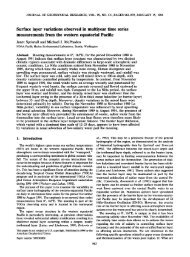
<strong>Internal</strong> <strong>Waves</strong> <strong>are</strong> <strong>all</strong> <strong>around</strong> <strong>us</strong>...<br />
Petrenko et al 00<br />
17-18 isotherms<br />
Baroclinic velocity<br />
Google Earth<br />
Eich et al 04
Erratic internal waves at SIO Pier<br />
data and wavelet analysis courtesy of E. Terrill, SIO<br />
Barotropic (depth-independent)<br />
Baroclinic (depth-dependent)<br />
semi-diurnal<br />
diurnal<br />
Time in hours<br />
Time in hours
Simple interfacial internal wave<br />
h = −h 0 cos(kx − ωt)<br />
2π/k = one wavelength<br />
U 1 = ωh 0<br />
cos(kx − ωt)<br />
H 1 k<br />
H 1<br />
U 1<br />
h<br />
U 2 = − ωh 0<br />
cos(kx − ωt)<br />
H 2 k<br />
H 2<br />
U 2<br />
after Gill,<br />
Atmosphere-Ocean Dynamics
Linearize equations of motion<br />
∂u<br />
= −⃗u · ∇u + fv − 1 ∂p<br />
∂t<br />
ρ ∂x + ν∇2 u<br />
∂v<br />
= −⃗u · ∇v − fu − 1 ∂p<br />
∂t<br />
ρ ∂y + ν∇2 v<br />
∂w<br />
= −⃗u · ∇w − 1 ∂p<br />
∂t<br />
ρ ∂z + ν∇2 w − g<br />
∂ρ<br />
∂t<br />
= −⃗u · ∇ρ + κ∇ 2 ρ<br />
∇ · ⃗u = 0<br />
<strong>Internal</strong> wave equations<br />
Low-mode vers<strong>us</strong> high-mode<br />
Try a solution of the form<br />
u(x, y, z, t) = ûe −i[kx+ly+mz−ωt]<br />
Get polarization and dispersion<br />
relationships<br />
ω 2 = (k2 + l 2 ) ∗ N 2 + m 2 ∗ f 2<br />
k 2 + l 2 + m 2<br />
Wave propagation direction<br />
U = Ψ(z)cos(kx − ωt)<br />
(Glenn Flierl)
What generates internal waves?<br />
1) Barotropic tide sloshing over topography<br />
<strong>Internal</strong> Tide: An internal wave<br />
with a tidal frequency, <strong>us</strong>u<strong>all</strong>y<br />
once in 12.4 hours = M2<br />
Often generated at the continental<br />
shelf break, with waves<br />
propagating both on and off<br />
shore.<br />
(J. Nash)
What generates internal waves?<br />
Spring Observations<br />
2) Wind makes near-inertial internal waves<br />
116 118 120 122 124 126 128 130<br />
! / N m !2<br />
0.4<br />
0.2<br />
Wind Stress<br />
0<br />
15<br />
8<br />
T<br />
z / m<br />
35<br />
7<br />
T / ° C<br />
55<br />
6<br />
V bc<br />
15<br />
S 2<br />
z / m<br />
z / m<br />
35<br />
55<br />
15<br />
30<br />
45<br />
0.2<br />
0<br />
!0.2<br />
!3<br />
!4<br />
!5<br />
!6<br />
log 10<br />
(S 2 / s !2 )<br />
V bc<br />
/ m s !1<br />
116 118 120 122 124 126 128 130<br />
yearday<br />
(MacKinnon and Gregg, JPO, Dec 05)
13 Dec 2003 18:52 AR AR203-FL36-12.tex AR203-FL36-12.sgm LaTeX2e(2002/01/18) P1: IBD<br />
<strong>Internal</strong> wave breaking mixes the ocean<br />
302 WUNSCH FERRARI<br />
<strong>Waves</strong> break by shear instability<br />
or convective overturning.<br />
Woods 68<br />
Wunsch and Ferrari 04<br />
Figure 5 Strawman energy budget for the global ocean circulation, with uncertainties of<br />
at least factors of 2 and possibly as large as 10. Top row of boxes represent possible energy<br />
sources. Shaded boxes <strong>are</strong> the principal energy reservoirs in the ocean, with crude energy<br />
values given [in exajoules (EJ) 10 18 J, and yottajoules (YJ) 10 24 J]. Fluxes to and from the<br />
reservoirs <strong>are</strong> in terrawatts (TWs). Tidal input (see Munk & Wunsch 1998) of 3.5 TW is<br />
the only accurate number here. Total wind work is in the middle of the range estimated by<br />
Lueck & Reid (1984); net wind work on the general circulation is from Wunsch (1998).<br />
Heating/cooling/evaporation/precipitation<br />
drive the global<br />
values <strong>are</strong> <strong>all</strong> taken<br />
meridional<br />
from Huang & Wang (2003).<br />
Value for surface waves and turbulence is for surface waves alone, as estimated by Lefevre<br />
& Cotton (2001). The internal overturning wave energy estimatecirulation<br />
is by Munk (1981); the internal tide<br />
energy estimate is from Kantha & Tierney (1997); the Wunsch (1975) estimate is four times<br />
larger. Oort et al. (1994) estimated the energy of the general circulation. Energy of the<br />
mesoscale is from the Zang & Wunsch (2001) spectrum (X. Zang, personal communication,<br />
2002). Ellipse indicates the conceivable importance of a loss of balance in the geostrophic<br />
mesoscale, resulting in internal waves and mixing, but of unknown importance. Dashed-dot<br />
lines indicate energy returned to the general circulation by mixing, and <strong>are</strong> first multiplied<br />
by Ɣ. Open-ocean mixing by internal waves includes the upper ocean.<br />
May provide enough total power to
Latitude / °<br />
Latitude / °<br />
50<br />
40<br />
30<br />
20<br />
10<br />
0<br />
-10<br />
-20<br />
-30<br />
-40<br />
50<br />
40<br />
30<br />
20<br />
10<br />
0<br />
-10<br />
-20<br />
-30<br />
-40<br />
50<br />
40<br />
30<br />
20<br />
10<br />
0<br />
-10<br />
-20<br />
-30<br />
-40<br />
50<br />
40<br />
30<br />
20<br />
10<br />
0<br />
-10<br />
-20<br />
-30<br />
-40<br />
JFM<br />
AMJ<br />
JAS<br />
OND<br />
Cant’ explicitly resolve internal waves in climate models.<br />
3 steps to parameterize their role:<br />
1) Wave generation<br />
1997<br />
<strong>Internal</strong>-Tide Generation<br />
-50<br />
0 50 100 150 200 250 300 350<br />
Longitude / °<br />
0.1 1 5 30<br />
10 3 Π() / Wm -2<br />
Egbert and Ray 01<br />
Wind-generated near-inertial internal waves<br />
Alford 01<br />
3058<br />
/ m<br />
Π(50 m) / mW m -2<br />
6<br />
4<br />
2<br />
0<br />
150<br />
100<br />
50<br />
0<br />
Π() / mW m -2<br />
3<br />
2<br />
1<br />
0<br />
a<br />
b<br />
c<br />
2) Wave<br />
ARTICLE<br />
propagation<br />
IN PRESS<br />
<strong>Internal</strong>-Tide Propagation<br />
37.5 N<br />
37.5 S<br />
J F M A M J J A S O N D<br />
Month<br />
Fig. 13. Baroclinic energy flux ^J and conversion rate ^C from our two-layer simulation, normalized according to (14) and<br />
one tidal cycle. Only a subset of the flux vectors <strong>are</strong> shown. The zonal mean of the normalization factor (Eq. (14) and Fi<br />
on the right side of the plot. Each vector component has been spati<strong>all</strong>y smoothed with a bidirectional Hanning window w<br />
to 2 degrees and then sub-sampled in order to give a meaningful large-scale picture of the general pattern and magnitude<br />
visual clarity it was necessary to make the color range representing the conversion rate be different from Fig. 12, to clip<br />
than 20 kW m 1 ; and to delete vectors shorter than 1 kW m 1 :<br />
Figure 6. (a,c) The monthly mean flux is<br />
plotted for each year 1996-1999 (thin lines,<br />
solid=1996,dashed=1997,dashdot=1998,dotted=1999),<br />
and for the 4-year mean (heavy line). Black lines <strong>are</strong> from<br />
37.5 ◦ N, and gray lines <strong>are</strong> from 37.5 ◦ S. (a) The flux<br />
without mixed-layer-depth correction, Π(50 m). (b) The<br />
The conversion is mostly positive (energy<br />
transfer is from barotropic to baroclinic motions),<br />
and in <strong>all</strong> of our regional estimates the net<br />
conversion is positive. However, over sm<strong>all</strong> spatial<br />
scales there <strong>are</strong> regions that <strong>are</strong> negative. For our<br />
two-layer simulations, the total barotropic-to-<br />
H.L. Simmons et al. / Deep-Sea Research II 51 (2004) 3043–3068<br />
3) Wave breaking ...<br />
We note that a number of the regio<br />
significant generators of baroclinic w<br />
been commented on previo<strong>us</strong>ly in the<br />
and a global picture with many similari<br />
can be found in Egbert and Ray (2001<br />
referred to as ER. The level of spatial d<br />
7
Statistical models of wave breaking<br />
“With three parameters I can fit an elephant”<br />
-Lord Kelvin<br />
Generated waves<br />
gener<strong>all</strong>y have large<br />
(vertical) scales and low<br />
frequencies<br />
Resolution of GCMs<br />
somewhere in between<br />
Breaking waves gener<strong>all</strong>y<br />
sm<strong>all</strong> (vertical) scale.<br />
Sm<strong>all</strong>-scale waves have<br />
the most shear.<br />
Black Box<br />
E low-mode<br />
Ambient Conditions:<br />
-stratification<br />
-latitude<br />
-mesoscale features<br />
‘Universal’ spectra<br />
Gargett et al 81<br />
(9)<br />
Dissipation<br />
rate ( ɛ )<br />
(4)<br />
(1)
organisms R E V I E W. LMost E T T Eof R Sthis mixing occurs<br />
26 MARCH<br />
where<br />
2004<br />
internal waves<br />
wav<br />
velocity fluctuations in the Pacific and Atlantic oceans between<br />
break, overturning the density stratification of the ocean and<br />
statistic<strong>all</strong>y steady, or varies slowly in time, the rate at which Wri<br />
Below<br />
Models<br />
Atlantic thermocline,<br />
of down-scale<br />
(26 N, 29 W):<br />
energy<br />
m 2:75 !<br />
transfer<br />
0:6 428 N and 28 S to extend that result to equatorial regions. We find<br />
(for<br />
breaking dissipates Experimental energy verification<br />
approximately equals the rate Dop at<br />
creating l wave 1 < patches ! < 6 cpd) of[21].<br />
turbulence. Predictions of the rate at which a strong latitude dependence of dissipation in accordance with<br />
the energy<br />
ed to These deep ocean observations (Fig. 1) exhibit a higher<br />
the predictions is transferred 3 . In ourfrom observations, large to dissipation sm<strong>all</strong> scales. rates This andequiv<br />
The<br />
internal waves dissipate 2,3 were confirmed earlier at midlatitudes<br />
4,5 . Here we present observations of temperature and<br />
scale<br />
umber degree of variability Wave-wave than one might Interactions<br />
anticipate for a<br />
<strong>all</strong>ows accompanying the dissipation mixing rate across1density to besurfaces expressed near the in Equator terms of<br />
Triad theory of weakly nonlinear wave-wave interactions<br />
func in<br />
ta sets universal spectrum. Moreover, the deviations from the<br />
wave<strong>are</strong> parameters.<br />
less Garrett-Munk than 10%<br />
To<br />
of<br />
check<br />
those empirical at<br />
their<br />
mid-latitudes spectrum numerical<br />
for a similar<br />
simulations,<br />
background<br />
of internal waves. Reduced mixing close to the Equator<br />
asso H<br />
velocity tailed (e.g.McComas GM h spectral power and Muller) laws form a pattern: they seem to<br />
Theory: fluctuations Energy transfer infrom the Pacific large toand sm<strong>all</strong>-scale Atlantic internal oceans waves between<br />
st list roughly f<strong>all</strong> upon a curve with negative slope in the x; y<br />
Wright willand have to Flatte be taken 3 formulated into account in annumerical wave-<br />
strong ∂U<br />
plane. We show in the next section that the predictions of<br />
E(m, ω) ∝ m −2 analytic<br />
ω −2 simulations model based of o<br />
428 N and 28 S to extend that result to equatorial regions. We find<br />
ocean dynamics—for example, in climate change experiments.<br />
alimit,<br />
Doppler shifting of evolving test waves by a background wave<br />
wave latitude<br />
T<br />
turbulence = ... dependence −theory U · ∇U <strong>are</strong> consistent of dissipation with this pattern. in accordance with<br />
The Doppler <strong>Internal</strong> waves shifting <strong>are</strong> generated produces in the aocean netwhen energy its stratification flux toward is<br />
ons<br />
be theap-predictions of the field.—In this section we assume that the internal wave<br />
scales—that<br />
∂tA wave turbulence 3 . In our formulation observations, for the internal dissipation wave rates and disturbed. Observed Unlikedissipation surface waves, rates which agree propagate with predictions,<br />
horizont<strong>all</strong>y<br />
beca<strong>us</strong>e they<br />
is,<br />
<strong>are</strong><br />
higher<br />
confined<br />
wavenumbers—and<br />
to the air–sea interface,<br />
ultimate<br />
internal waves<br />
breaking term<br />
accompanying<br />
field<br />
U<br />
can<br />
=<br />
be<br />
mixing Uviewed 1 e i(k 1·x−ω<br />
across 1<br />
as a field t) density +<br />
ofU weakly 2 e i(k surfaces<br />
2·x−ω 2<br />
interacting<br />
t) + near U 3 ethe i(k 3·x−ω<br />
Equator 3 t) + ... based on measurements of shear and strain. (Gregg F<br />
functional str<br />
propagate dependence vertic<strong>all</strong>y as well of 1 as(which horizont<strong>all</strong>y, is expressed making flowindisturb-<br />
ances89, at the Polzin surface et oral bottom 95)<br />
Stra<br />
units of<br />
waves, th<strong>us</strong> f<strong>all</strong>ing into the class of systems describable<br />
W<br />
<strong>are</strong> less than 10% of those at mid-latitudes for a similar backgroundenergy<br />
and Munk<br />
felt in the interior. Garrett and Munk 6<br />
(2)<br />
associated with this flux is the product of two terms:<br />
by wave turbulence. Wave turbulence is a universal<br />
dens<br />
fficient<br />
Eikonal<br />
of internal transfer<br />
statistical calculations<br />
waves. through<br />
theory for the of sm<strong>all</strong>-scale<br />
Reduced resonant<br />
description ofwaves mixing triads:<br />
an ensemble propagating<br />
close to the Equator<br />
7 modelled internal waves in terms of a wavenumber–<br />
of<br />
men<br />
is its<br />
frequency spectrum; they assumed that the wave field is constant in<br />
will have through weakly to be spectrum interacting taken particles of into larger account or waves. in This (Henyey numerical theoryet has<br />
obse<br />
al) simulations of<br />
1 ¼ 1 308 N; F shear ðmÞ; F strain ðmÞ £ Lðv; NÞ<br />
0 is a<br />
k<br />
contributed to our 1 = k<br />
understanding 2 + k 3 ω<br />
of spectral 1 = ω<br />
energy 2 + ω 3<br />
depe<br />
ocean dynamics—for example, in climate change experiments.<br />
transfer in complex systems [22], and has been <strong>us</strong>ed for<br />
The first term, 1 at the 308 GM model reference latitude, de<br />
waves, it <strong>Internal</strong> I: Continuo<strong>us</strong> describing waves Steady surface spectrum <strong>are</strong> flux generated water to sm<strong>all</strong>er waves of waves insince the vertical pioneering ocean when scales worksits stratification is<br />
ormed<br />
on stratification (via N) and on internal wave characteristi<br />
disturbed. by Hasselmann Unlike surface [23], Benney waves, and which Newell [24], propagate and horizont<strong>all</strong>y<br />
wavey<br />
the they <strong>are</strong> confined to the air–sea interface, internal waves<br />
eragingZakharov over randomly [25,26]. distributed terms of spectra of vertical shear, F shear (m), and of vertical<br />
beca<strong>us</strong>e<br />
The dynamics F of ∝oceanic Ê2 wave<br />
internal N 2 phases and directions leads to slow, ineffint<br />
energy easily transfers, vertic<strong>all</strong>y describede.g. in asisopycnal months well as(i.e., horizont<strong>all</strong>y, to density) transfercoordinates,<br />
energy making out of flow a mode-one disturb-internal tide<br />
waves can be most<br />
F<br />
propagate m,<br />
strain (m), where m is the vertical wavenumber in cycles per m<br />
Strain fluctuations <strong>are</strong> variations of the vertical separations be<br />
ances atwhich the surface<br />
<strong>all</strong>ow foror a simple<br />
bottom<br />
andfelt intuitive the<br />
Hamiltonian<br />
interior.<br />
description<br />
[12]. 82, Muller To describe et al 86] the wave field, we introduce<br />
density surfaces, that is, fluctuations of ›z/›z. Previo<strong>us</strong> me<br />
lbers and Pomphrey Garrett and Munk 6<br />
and Munk Theoretic<strong>all</strong>y predicted ‘family’ of steady-state<br />
two 7 variables: modelled a velocity internal potential waves r; inand terms an isopycnal<br />
spectrum; straining ...hamiltonian....<br />
4 verified the shear and N dependence in 1 308 , and subse<br />
of a wavenumber– ments<br />
frequency spectra<br />
it II: Distinct individual<br />
r; they . The<br />
waves assumed horizontalthat velocity theiswave given by field is constant in<br />
the isopycnal gradient r of the velocity potential,<br />
observations 5 and numerical simulations 8 confirmed the<br />
m:<br />
dependence. The second term contains the latitude (v) depen<br />
nsider a coherent internal A(m, k) tide. ∝ mExplore −y k −x basic physics with idealized numerical<br />
2.5<br />
ertical<br />
NATRE<br />
2<br />
Lðv; NÞ ¼<br />
f cosh21 ðN=f Þ<br />
periments, in both nearfield and farfield of wave generation sites...<br />
f 308 cosh 21 ðN 0 Gregg =f 308 Þ03<br />
major<br />
ur best<br />
uency<br />
ODE),<br />
0 0 W):<br />
servaa<br />
ther-<br />
].<br />
EX),<br />
cline,<br />
riment<br />
a ther-<br />
y−power law of 3−d action spectrum<br />
1.5<br />
1<br />
0.5<br />
0<br />
−0.5<br />
−1<br />
energy equipartition<br />
Eq.(5)<br />
FASINEX<br />
AIWEX<br />
PATCHEX<br />
MODE<br />
IWEX<br />
−1.5<br />
0 0.5 1 1.5 2 2.5 3 3.5 4 4.5 5<br />
x−power law of 3−d action spectrum<br />
GM<br />
SWAPP<br />
Lvov et al 04<br />
ONR – p.4<br />
Figure 1 Reduction of dissipation rates produced by breaking internal waves near the<br />
Equator. The predicted latitude effect L is unity at 308 beca<strong>us</strong>e the standard internal wave<br />
spectrum, Garrett and Munk 6 , and the calculations based on it <strong>are</strong> referenced to that<br />
latitude. Ratios of average 1 observed to 1 308 <strong>are</strong> plotted as short horizontal bars, and upper<br />
and lower 95% confidence limits <strong>are</strong> shown by extents of the vertical lines. Multiple values<br />
at the same latitude v come from different depths or locations. The shaded curve gives the<br />
predicted L(v,N) for the range of N encountered. Beca<strong>us</strong>e the N dependence is weak, the<br />
height of the shaded band is sm<strong>all</strong>. Upper and lower solid lines <strong>are</strong> twice and one-half the<br />
prediction, and approximately bound the scatter in the data. In spite of the scatter, the<br />
observations confirm the predicted sharp cut-off of dissipation at low latitude.<br />
Numerical simulations of internal-wave interactions.<br />
Confirm GM spectrum as steady state and predicted<br />
rates of down-scale energy flow. ( Hibiya et al,<br />
Winters and D’Asaro, etc)<br />
Figur<br />
strati<br />
latitud<br />
the la<br />
the E<br />
water
n water masses of uniform density than across<br />
g waters of different densities. But the magnition<br />
of mixing across density surfaces <strong>are</strong> also<br />
Earth’s climate as well as the concentrations of<br />
t of this mixing occurs where internal waves<br />
ng the density stratification of the ocean and<br />
of turbulence. Predictions of the rate at which<br />
dissipate 2,3 were confirmed earlier at midwe<br />
present observations of temperature and<br />
ons in the Pacific<br />
Sources<br />
and Atlantic oceans between<br />
extend that result to equatorial regions. We find<br />
dependence of dissipation in accordance with<br />
. In our observations, dissipation rates and<br />
- low mode<br />
- estimate from observations<br />
50<br />
40<br />
6<br />
30<br />
1997<br />
a<br />
20 JFM<br />
10<br />
0<br />
4<br />
ixing-10<br />
- explicitly<br />
across density<br />
-20 resolve<br />
surfaces<br />
in GCM<br />
near the<br />
(?)<br />
Equator<br />
-30<br />
-40<br />
2<br />
50<br />
40<br />
30<br />
0<br />
20<br />
b<br />
10<br />
AMJ<br />
150<br />
aken into 0 account in numerical simulations 100 of<br />
-10<br />
-20<br />
50<br />
-30<br />
for example, 0<br />
-40<br />
in climate change experiments.<br />
Latitude / °<br />
50<br />
40<br />
3<br />
30<br />
20<br />
10<br />
JAS<br />
2<br />
surface 0 waves, which propagate horizont<strong>all</strong>y<br />
-10<br />
-20<br />
1<br />
-30<br />
-40<br />
Latitude / °<br />
50<br />
40<br />
30<br />
20<br />
10<br />
OND<br />
0<br />
-10<br />
-20<br />
-30<br />
-40<br />
-50<br />
0 50 100 150 200 250 300 350<br />
Longitude / °<br />
0.1 1 5 30<br />
10 3 Π() / Wm -2<br />
Figure 5. Season<strong>all</strong>y averaged maps of energy flux from<br />
the wind into near-inertial mixed-layer motions for the year<br />
1997. Variability in mixed-layer depth is included by season<strong>all</strong>y<br />
averaging the Levit<strong>us</strong> climatology.<br />
and the model gives zero currents. A few (< 1%) season<strong>all</strong>yaveraged<br />
values <strong>are</strong> < 0 (loss of energy to the atmosphere),<br />
but <strong>all</strong> of these have magnitudes less than 0.1 mWm −2 , and<br />
so <strong>are</strong> also plotted in blue. The rough land edges reflect the<br />
2.5 ◦ grid spacing.<br />
◦<br />
/ m<br />
Π(50 m) / mW m -2<br />
Π() / mW m -2<br />
c<br />
Doppler shifting of evolving 7 test waves by a background wave field.<br />
37.5 N<br />
scales—that is, higher 37.5 S wavenumbers—and ultimate breaking. The<br />
Figure 6. (a,c) The monthly mean flux is<br />
plotted for each year 1996-1999 (thin lines,<br />
solid=1996,dashed=1997,dashdot=1998,dotted=1999),<br />
and for the 4-year mean (heavy line). Black lines <strong>are</strong> from<br />
37.5 ◦ N, and gray lines <strong>are</strong> from 37.5 ◦ S. (a) The flux<br />
without mixed-layer-depth correction, Π(50 m). (b) The<br />
monthly mean, zon<strong>all</strong>y averaged Levit<strong>us</strong> and Boyer [1994]<br />
mixed layer depth, < H >, at 37.5 ◦ N (black) and 37.5 S<br />
(gray). (c) Mixed-layer-depth corrected flux, Π(H).<br />
4.2. Seasonal Cycle<br />
Wave propagation<br />
through resolved mesoscale<br />
(4)<br />
(1)<br />
But the problem is that there <strong>are</strong> some exceptions where f 308 cosh wave 21 ðNenergy 0 =f 308 Þ doesn’t<br />
cascade in this nice way, and<br />
the importance<br />
these<br />
of the inertial<br />
exceptions,<br />
component of the windthough fields,<br />
localized, might dominate<br />
rather than their over<strong>all</strong> magnitude, in generating near-inertial<br />
mixing in key places. Best motions. to ill<strong>us</strong>trate through examples...<br />
(9)<br />
Wave breaking<br />
(sm<strong>all</strong> scales)<br />
E t ( ⃗ k, ⃗x, t) = S o (k) − ∇statistic<strong>all</strong>y x · (C<br />
steady, or<br />
g E)<br />
varies−slowly ∇in time,<br />
k · F<br />
the<br />
(k)<br />
rate at which<br />
− Swave<br />
i (k)<br />
of those at mid-latitudes for a similar backal<br />
waves. Reduced mixing close to the Equator<br />
re generated in the ocean when its stratification is<br />
confined to the air–sea interface, internal waves<br />
0<br />
lly as well as horizont<strong>all</strong>y, making flow disturb-<br />
J F M A M J J A S O N D<br />
Month<br />
e or bottom felt in the interior. Garrett and Munk 6<br />
lled internal waves in terms of a wavenumber–<br />
m; they assumed that the wave field is constant in<br />
significantly more energetic.<br />
Numerical simulations of energy transfer by interactions within<br />
the internal wave field show a net flux Spectral towards flux sm<strong>all</strong> spatial scales<br />
that increases the shear variance (›u/›z) (down-scale)<br />
2 until it overcomes the<br />
stratification and the waves break 2,3 . When the wave field is<br />
breaking dissipates energy approximately equals the rate at which<br />
the energy is transferred from large to sm<strong>all</strong> scales. This equivalence<br />
<strong>all</strong>ows the dissipation rate 1 to be expressed in terms of internal<br />
wave parameters. To check their numerical simulations, Henyey,<br />
Wright and Flatte 3 formulated an analytic model based on the<br />
}<br />
Parameterize unresolved dissipation rate as rate<br />
of down-scale energy transfer to IW continuum<br />
The Doppler shifting produces a net energy flux toward sm<strong>all</strong>er<br />
functional dependence of 1 (which is expressed in units of W kg 21 )<br />
associated with this flux is the product of two terms:<br />
1 ¼ 1 308 N; F shear ðmÞ; F strain ðmÞ £ Lðv; NÞ ð1Þ<br />
The first term, 1 at the 308 GM model reference latitude, depends<br />
on stratification (via N) and on internal wave characteristics (in<br />
terms of spectra of vertical shear, F shear (m), and of vertical strain,<br />
F strain (m), where m is the vertical wavenumber in cycles per metre).<br />
Strain fluctuations <strong>are</strong> variations of the vertical separations between<br />
density surfaces, that is, fluctuations of ›z/›z. Previo<strong>us</strong> measurements<br />
4 verified the shear and N dependence in 1 308 , and subsequent<br />
observations 5 and numerical simulations 8 confirmed the strain<br />
dependence. The second term contains the latitude (v) dependence:<br />
Lðv; NÞ ¼<br />
f cosh21 ðN=f Þ<br />
ð2Þ
Problem I: Fast wave interactions<br />
Parametric Subharmonic Instability (PSI): Decay of a initial wave (e.g. low-mode<br />
internal tide), into two sm<strong>all</strong>er-scale waves of half the frequency. Seems to be<br />
particularly efficient/resonant when the subharmonic frequency is equal to the local<br />
intertial frequency (28.9 N/S).<br />
Display Image<br />
Numerical evidence for fast PSI near 29<br />
Close Print<br />
[next]<br />
02/27/2006 12:45 PM<br />
MacKinnon and Winters 05<br />
FIG. 1. Time variations of the energy spectrum at (a) 49°, (b) 28°, and (c) 18°N in the two-dimensional<br />
wavenumber space after the injection of the lowest-vertical-wavenumber M 2 internal tide energy. Note that each<br />
spectrum is scaled by the unforced, freely decaying, reference spectrum. The red triangle at the lower left in each<br />
panel shows the spectral location of the lowest-vertical-wavenumber M 2 internal tide. Numerals on the solid lines<br />
denote the wave period.<br />
Furuichi et al 05
JANUARY 2006 T I A N E T A L . 41<br />
Observational evidence for something special near 29<br />
‘Dissipation rate’ of internal tide, as inferred from convergences in internal tide<br />
energy fluxes measured with satellite altimetry.<br />
Atlantic Ocean<br />
Indian Ocean<br />
JANUARY 2006 T I A N E T A L . 41<br />
JANUARY 2006<br />
Pacific Ocean<br />
T I A N E T<br />
2 -1<br />
Inferred diff<strong>us</strong>ivity / m s<br />
FIG. 9. Latitudinal distribution of the mixing rate ca<strong>us</strong>ed by M 2<br />
internal tides in (a) the Pacific, (b) the Atlantic, and (c) the Indian<br />
Oceans.<br />
Latitude Latitude Latitude<br />
large as 50 m, the relative error of the dissipation rate<br />
would still be no larger than 20%.<br />
The calculations <strong>are</strong> based on 10 years of TOPEX/<br />
Poseidon altimeter tidal data. The nominal bias of tidal<br />
data is 1.5 cm (Benada 1997). The wavenumber of baroclinic<br />
M 2 internal tides is of the order of 0.01 km 1 , the<br />
average depth of the thermocline is assumed to be 500<br />
m, and the average water depth is about 4000 m. The<br />
estimated bias of the energy flux in Fig. 6 is about 1000<br />
W m 1 . We also estimate the error ca<strong>us</strong>ed by the nomi-<br />
FIG. 9. Latitudinal distribution of the mixing rate ca<strong>us</strong>ed by M 2<br />
internal tides in (a) the Pacific, (b) the Atlantic, and (c) the Indian<br />
Oceans.<br />
There <strong>are</strong> some volumes in which the fluxes <strong>are</strong> insufficient<br />
to calculate the summation. There <strong>are</strong> also a<br />
few volumes near large topography, for example, near<br />
the east of A<strong>us</strong>tralia, in which the sum of fluxes is negative.<br />
This means that Eq. (4) does not apply in such<br />
<strong>are</strong>as and, as a consequence, not <strong>all</strong> energy fluxes in Fig.<br />
6 <strong>are</strong> <strong>us</strong>ed to calculate the energy dissipation shown in<br />
Fig. 7.<br />
The error is as large as one-quarter of the mixing rate<br />
ca<strong>us</strong>ed by M 2 internal tides near 28.9°N/S and is even<br />
Tian et al 06:<br />
(suggestive blue lines added by me)<br />
i<br />
O
Observational evidence for fast PSI near 29<br />
<strong>Internal</strong> <strong>Waves</strong> Across the Pacific (IWAP)<br />
Alford, Klymak, MacKinnon, Munk, Pinkel<br />
38<br />
36<br />
Altimetry<br />
2 kW/m<br />
PEZHAT<br />
2 kW/m<br />
Mooring<br />
MP6<br />
TOPEX<br />
Pass 249<br />
TOPEX<br />
<br />
Filtered <br />
Velocity at the ‘critical’ latitude<br />
2 kW/m<br />
34<br />
32<br />
MP5<br />
Neap<br />
TS2<br />
Latitude<br />
30<br />
TS1<br />
MP4<br />
28<br />
MP3<br />
MP2<br />
TS3<br />
26<br />
24<br />
MP1<br />
Spring<br />
-16 -8 0 8<br />
/ cms -1<br />
Average near-inertial kinetic energy vs. latitude<br />
22<br />
Fench Frigate Shoals<br />
Nihoa Island<br />
Kauai Channel<br />
-14.4 -7.2 0 7.2<br />
SSHA / cm<br />
192 194 196 198 200 202 204<br />
Longitude<br />
-6 -4 -2 0<br />
Depth / 1000 m<br />
ure 1: (Left) Bathymetry (colors; axis at lower right), measurement locations (black = moors;<br />
blue = shipboard time series; white = ship track), and internal-tide energy fluxes (yellow<br />
}
38<br />
36<br />
Altimetry<br />
2 kW/m<br />
PEZHAT<br />
2 kW/m<br />
Mooring<br />
2 kW/m<br />
MP6<br />
TOPEX<br />
Pass 249<br />
Problem II: coherent waves<br />
TOPEX<br />
<br />
Filtered <br />
34<br />
32<br />
MP5<br />
Neap<br />
East-west sections of inerti<strong>all</strong>y back-rotated velocity<br />
TS2<br />
Latitude<br />
30<br />
TS1<br />
MP4<br />
28<br />
TS3<br />
MP3<br />
MP2<br />
26<br />
Spring<br />
24<br />
MP1<br />
-16 -8 0 8<br />
/ cms -1<br />
22<br />
Fench Frigate Shoals<br />
Nihoa Island<br />
Kauai Channel<br />
-14.4 -7.2 0 7.2<br />
SSHA / cm<br />
192 194 196 198 200 202 204<br />
Longitude<br />
-6 -4 -2 0<br />
Depth / 1000 m<br />
: (Left) Bathymetry (colors; axis at lower right), measurement locations (black = moore<br />
= shipboard time series; white = ship track), and internal-tide energy fluxes (yellow<br />
AT numerical model; black=altimetry; red = moorings). Reference arrows <strong>are</strong> at upper<br />
the critical latitude, 28.8 o N, is indicated with a dotted line. Note the PEZHAT model<br />
nds at 32 o N. Moored flux variability is indicated with gray curves, which enclose the<br />
ly 50% of observed values. (Right) Raw (blue) and highpass-filtered (red) meridional<br />
averaged from 0-1000 m depth on a southward transit from MP6 to MP1 at yearday<br />
ce the transit took 4.5 days to complete, the ship passed through northbound modegenerated<br />
at Hawaii’s neap tide near 33 o N, and at the following spring tide at 26 o N<br />
t left). SSHA from TOPEX/POSEIDON track 249 (plotted at left, black) is overplotted<br />
ip reference frame (black; see text). The axis limits for 〈V 〉 and SSHA (shown below)<br />
l for a mode-1 free wave.<br />
4<br />
North-south section of back-rotated velocity
Problem III - internal tide ‘directly breaks’<br />
Hawaiian Ocean Mixing Experiment (HOME)<br />
Huge overturns as internal tide sloshes<br />
up and down a steep slope<br />
Levine and Boyd 06<br />
Aucan et al 05<br />
Dissipation rate<br />
FIG. 1. R/P FLIP was moored in 1100 m of water over K<br />
N, 158 ◦ 37.77 ′ W. Also shown <strong>are</strong> two moorings from the sa<br />
larger near-bottom overturns have been observed.<br />
Velocity<br />
Temperature<br />
Klymak et al 07
Problem III - internal tide ‘directly breaks’<br />
Hawaiian Ocean Mixing Experiment (HOME)<br />
Huge overturns as internal tide sloshes<br />
up and down a steep slope<br />
Levine and Boyd 06<br />
Aucan et al 05<br />
Dissipation rate<br />
Gregg-Henyey parameterization works in<br />
upper water column, but not for the<br />
deeper, stronger mixing.<br />
FIG. 1. R/P FLIP was moored in 1100 m of water over K<br />
N, 158 ◦ 37.77 ′ W. Also shown <strong>are</strong> two moorings from the sa<br />
larger near-bottom overturns have been observed.<br />
Velocity<br />
Temperature<br />
Klymak et al 07
Directly breaking internal tide on Oregon slope<br />
Similarly huge overturns, but in a<br />
place not predicted by global<br />
internal tide generation maps.<br />
L01605<br />
L01605 NASH ET AL.: MIXING HOTSPOTS L01605<br />
profiler and shipboard CTD yields the turbulent dissipation<br />
rate i = 0.64L 2 Ti N 3 i , where N i and L Ti represent the<br />
Thorpe-resorted stratification and rms Thorpe displacement<br />
for the ith overturning region [Dillon, 1982]. Each L Ti is<br />
rejected if sm<strong>all</strong>er than the expected (spurio<strong>us</strong>) values for<br />
depth and density imprecision [Alford et al., 2006]. Following<br />
Gregg [1989] and Gregg and Kunze [1991], was<br />
parameterized from XCP data and found consistent with<br />
Thorpe estimates at stations where XCP and CTD measurements<br />
coincided (stations 3.3, 4.3 and 5.3). For both<br />
overturn and Gregg-Henyey , diff<strong>us</strong>ivity was computed<br />
as K r = 0.2N 2 [Osborn, 1980].<br />
3. Observations<br />
[11] High near-bottom turbulent energy dissipation rates<br />
span the 20-km region of enhanced roughness (Figure 2,<br />
43.21° N, 125.05–125.3° W). Within 500 mab, timeaverage<br />
K r were 10 4 –10 3 m 2 /s above rough topography,<br />
NASH ET AL.: MIXING HOTS<br />
Nash et al 07<br />
Figure 3. Timeseries at LADCP/CTD station L2.5 at the<br />
2200-m isobath (first occupation): (a) observed (blue) and<br />
with the r<br />
observed<br />
and Boyd<br />
[13] Up<br />
(and henc<br />
velocity b<br />
northward<br />
(i.e., x = R<br />
the large-s<br />
and orien<br />
during th<br />
dissipation<br />
near-botto<br />
forms the<br />
dissipation<br />
However,<br />
is the sam<br />
vertical w<br />
generation<br />
[Baines, 1<br />
[14] At<br />
lence ( <br />
during bo<br />
5 days; 3<br />
eastern ed<br />
green), w<br />
this statio<br />
the 2200-<br />
within 15
Problem IV: Solitons (internal waves of un<strong>us</strong>ual size)<br />
nonlinear steepening<br />
balanced by disperson<br />
24 hours<br />
Stanton and Ostrovsky<br />
GRL 24(14) 1998<br />
100 minutes
2106 J O U R N A L O F P H Y S I C A L O C E A N O G R A P H Y<br />
VOLUME 33<br />
period. (b), (d) Same for interval surrounding yearday 238.96.<br />
Extreme soliton breaking<br />
thermocline on yearday 238 and depth between 20 and<br />
40 m during yearday 242 (Fig. 4). Other patches of high<br />
diff<strong>us</strong>ivity were associated with anomalo<strong>us</strong>ly low stratification<br />
but not with elevated dissipation, such as above<br />
profiles of turbulent dissipation rate. The spacing of the<br />
dissipation profiles ill<strong>us</strong>trates the degree to which ou<br />
profiler undersampled the event. The locations of two<br />
reference isopycnals that bound the thermocline <strong>are</strong><br />
shown for each profile. Average dissipation within thi<br />
density range remained <strong>around</strong> 10 6 W kg 1 in the third<br />
through seventh profiles (until minute 30), then de<br />
FIG. 14. Example aco<strong>us</strong>tical snapshot of a propagating ISW within which is embedded a sequence of rollups identical in nature to Kelvin–<br />
Helmholtz instabilities observed in the laboratory and in sm<strong>all</strong>-scale simulations. The vertical scale of the largest is more than 10 m, and<br />
the horizontal scale Moum (in the direction et ofal wave 03 propagation) is about 50 m. Toward the trailing edge of the wave, the rollups become less<br />
coherent but contribute a greater backscatter signal, suggesting breakdown to turbulence. At greater depth, denoted by arrows, <strong>are</strong> two more<br />
layers of bright backscatter. These <strong>are</strong> presumably the same phenomenon, but sm<strong>all</strong>er scale. Hence the echosounder resolution does not<br />
permit a clear depiction of rollups.<br />
given the density profile at the same location. First, the<br />
ambient streamfunction in the wave’s reference frame<br />
is obtained from the measured upstream velocity profile<br />
u 0 (z) <strong>us</strong>ing<br />
z<br />
0<br />
(z) [u (z) c ] dz. (3)<br />
0 <br />
w<br />
50-75 % of total average<br />
daily mixing occurs in<br />
these few minutes<br />
At any location within the wave, we obtain the streamfunction<br />
profile corresponding to the local density profile<br />
1 (z) <strong>us</strong>ing<br />
( ) ( ).<br />
1 1 0 0 (4)<br />
Last, we differentiate 5 to obtain the velocity profile and<br />
transform into the earth’s reference frame:<br />
1<br />
u 1 c w . (5)<br />
z<br />
An appropriate value for was obtained by examining<br />
density fluctuations in six profiles prior to and<br />
including the profile selected for analysis. Thorpe reordering<br />
was <strong>us</strong>ed to estimate density fluctuations in<br />
turbulent overturns. The maximum fluctuation had absolute<br />
value of 0.1 kg m 3 (Fig. 17). We adopted this<br />
MacKinnon and Gregg 03<br />
FIG. 10. The solid lines <strong>are</strong> contours of northward (onshelf) baroclinic velocity from 0.3 to 0.3 m s 1 in intervals of 0.1 m s 1 . Th<br />
shaded <strong>are</strong>as <strong>are</strong> 4-m shear variance, ranging from 0 (white) to 3.5 10 3 s 2 (black) in increments of 5 10 4 s 2 . Profiles of dissipatio<br />
rate <strong>are</strong> overlain, and correspond to the colorbar above. The slight slant of each profile represents the passage of time as the profiler descends<br />
The black (upper) and magenta (lower) stars on each profile indicate the evolving locations of the 22.65 and 24 kg m 3 isopycnals, respectively<br />
Solitons <strong>around</strong> the world<br />
FIG. 15. (left) Observed profiles of horizontal velocity from 300-<br />
kHz ADCP (2-m bin size) and (right) from Chameleon. These<br />
coincide with the Chameleon profile noted by the black dot in Fig.<br />
9 which corresponds to the time of maximum stratification at the<br />
interface at 30-m depth, after which overturns and intense turbulence<br />
first appear.<br />
5<br />
Differentiations and integrations were approximated <strong>us</strong>ing second-order,<br />
finite differences on an uneven grid. Interpolations between<br />
the vario<strong>us</strong> data grids were done <strong>us</strong>ing an equal mixture of<br />
linear and cubic Hermite interpolants. (This controls the spurio<strong>us</strong><br />
peaks that appear when cubic interpolation is <strong>us</strong>ed alone.)<br />
Apel et al 06
ligible shear. Starting with this simple motion field, the goal is to predict its spectral<br />
Is the spectrum a myth? (the personalist approach)<br />
ature in s-L and Eulerian frames.<br />
Real-world observations depart from the “N-frame” ideal through advective<br />
Doppler shifting makes for broadened<br />
frequency band at higher wavenumbers.<br />
cts, which appear as phase distortions of the signal of interest: ie<br />
Arctic data<br />
38 38<br />
38<br />
s Eul = s 0 exp(i k*x + k*(V t) - ! t) 1)<br />
Normalized<br />
Intrinsic<br />
There<br />
shear<br />
<strong>are</strong><br />
only<br />
four<br />
at<br />
cases<br />
inertial<br />
to<br />
and<br />
consider:<br />
vortical (f=0)<br />
frequencies, advected by horizontal currents<br />
Sm<strong>all</strong> vs large phase distortion (! | k * V | dt > / < ")<br />
Stochastic vs deterministic distortion velocity, V<br />
Garrett-Munk<br />
The models introduced here relate the probability density function and / or the<br />
ctrum of the advecting velocity field, V, to the spectrum of the observed quantity. The<br />
roach follows a path suggested by Papoulis, 1984.<br />
The foc<strong>us</strong> is on the temporal<br />
Figure 2 a. A wavenumber-frequency spectrum of Arctic Ocean shear estimated from the<br />
SHEBA Doppler sonar. The white rectangle indicates the smoothing <strong>us</strong>ed to to to achieve 150<br />
degrees of freedom. The left quadrants of the spectrum correspond Pinkel to to to 07<br />
anti-cyclonic<br />
rotation in time. The lower left and upper right quadrants represent upward phase<br />
propagation, which for the internal wave component of the shear implies downward<br />
energy propagation.<br />
b. The associated normalized spectrum N(! z , ! z , z , ")=E(! z , ")/ ! E(! z , ") d". First<br />
(white) and second (black) spectral moments <strong>are</strong> indicated. Color contours mimic a<br />
“hourglass” pattern.<br />
covariance function, R(#), which, for a line spectral process (in the N-frame), takes<br />
form<br />
Perhaps the internal-wave continuum is<br />
in the eye of the beholder, at least the<br />
high-wavenumber part where <strong>all</strong> the<br />
shear lives.<br />
Doppler model
Concl<strong>us</strong>ions?<br />
Statistical models of internal-wave breaking <strong>are</strong> based on rates of down-scale<br />
energy transfer through steady, ga<strong>us</strong>sian fields of incoherent waves. Such<br />
models appear to work some places, but many of these <strong>are</strong> ‘boring’ places.<br />
In other places, mixing is dominated by extreme events, mostly beca<strong>us</strong>e ‘special<br />
physics’ is taking place.<br />
How much do extreme events matter?<br />
Coastal ocean - probably quite a bit, in sh<strong>all</strong>ow water<br />
most internal wave breaking is abnormal.<br />
Open ocean - hard to say. Factor of 2 near hawaii,<br />
averages out to not much basin-wide. But perhaps<br />
extreme breaking events <strong>are</strong> undersampled.
mber or frequency properties (P95).<br />
3) The wavenumber of the test waves also<br />
f waves is assumed to Breaking slowly evolve internal waves<br />
simply related to observed large-scale mo<br />
ratification and total wavefield energy<br />
cording to WKB theory, horizontal waven<br />
cal wavenumber of test waves depends<br />
does not change in Na stratification field<br />
al energy level. Specific<strong>all</strong>y, it is choroude<br />
spectra integrated out to a near-<br />
(Stratification)<br />
varies in the vertical. We therefore als<br />
Even if you can’t directly see turbulence, characteristic horizontal wavenumber in<br />
ber is order 1. Plugging in the anacan<br />
parameterize turbulent mixing in unknown constant.<br />
GM spectrum and the dispersion reree<br />
factors terms onof the observed rhs of (low-resolution)<br />
(6) can be With these( <strong>Internal</strong> assumptions,<br />
S<br />
)<br />
the three terms in (<br />
Wave<br />
ε<br />
Black<br />
her in such a way internal-wave that at a particular shear.<br />
Box<br />
Shear (9)<br />
(<br />
Turbulent<br />
ation rate scales as<br />
<br />
dEˆ<br />
<br />
E )<br />
0 N<br />
1488 J O U R N A L O F P H Y S I C A L O C E A N O G R A P H Y<br />
VOLUME 33 <br />
<br />
Dissipation<br />
dm<br />
(1)<br />
m<br />
(4)<br />
ˆ<br />
N 2<br />
0 N0<br />
2 1<br />
f E<br />
<br />
(W kg ), (7)<br />
2<br />
2<br />
N 0<br />
dU<br />
<br />
Slf<br />
S<br />
<br />
erence buoyancy frequency and f is<br />
dz<br />
0<br />
S 0<br />
ency (G89).<br />
kH<br />
k H0.<br />
s scaling with oceanic measurements<br />
dlatitude locations, G89 <strong>us</strong>es the ratio The product of <strong>all</strong> three terms gives a dissi<br />
at a fixed wavenumber (10 m) to the estimate that we will refer to as the MacKinn<br />
Munk shear at that scale as a proxy (M–G) scaling<br />
nergy level to get what we will sub-<br />
FIG. 13. (a) Observed dissipation data averaged in bins of 4-m stratification (x axis) and 4-m shear variance (y axis). The<br />
boundary of 4-m Richardson number 0.25 is shown for reference. (b), (c) Same as for the the Gregg–Henyey and MacKinnon–<br />
Gregg parameterizations, respectively.<br />
as the Gregg–Henyey (G–H) scaling,<br />
observed dissipation rate. Nevertheless, the shear and<br />
4 2<br />
H model dissipation rate has an inverse relationship with<br />
0 <br />
0 0<br />
N Slf<br />
1<br />
MG<br />
(W kg )<br />
N S
<strong>are</strong> we missing mixing still?<br />
Program/<br />
Experiment<br />
C - S A L T /<br />
SFTRE<br />
Diff<strong>us</strong>ivities<br />
O(×10 -4 ) m 2 /s<br />
0.1 (above/below stairs)<br />
1 (in staircase)<br />
Notes<br />
Double-diff<strong>us</strong>ive<br />
staircase<br />
PATCHEX 0.1 (thermocline) Thermocline<br />
processes<br />
Tropic Heat 1/<br />
Tropic Heat 2<br />
NATRE<br />
BBTRE<br />
0.1 (in thermocline)<br />
1 (in undercurrent)<br />
0.1 (thermocline)<br />
1 (in NADW)<br />
0.1 (in thermocline)<br />
1 (in NADW)<br />
>10 (in AABW)<br />
Equatorial<br />
processes<br />
First open-ocean<br />
tracer release<br />
Basin-scale<br />
survey<br />
ec 2003 18:52 AR AR203-FL36-12.tex HOME AR203-FL36-12.sgm 0.1 (away LaTeX2e(2002/01/18) from ridge) P1: Energy IBD budget<br />
1 (near the ridge) study<br />
288 WUNSCH FERRARI<br />
TABLE 1 Spatial-average across-isopycnal diff<strong>us</strong>viities, as estimated by vario<strong>us</strong><br />
budget methods. In the first six rows, the bottom region lies between neutral surface 28.1<br />
and the sea floor (see Figure 1), and from 27.96 to 28.07 for the deep layers. Gener<strong>all</strong>y,<br />
these lie between about 3800 m and the sea floor, and between about 2000 m and 3800 m,<br />
respectively, but with considerable spatial variations. The last six estimates <strong>are</strong> from<br />
restricted basins or channels, but <strong>all</strong> values <strong>are</strong> spatial averages over the interior and<br />
boundary layers<br />
Ocean/Depth 〈K 〉 (10 −4 m/s) Reference<br />
Atlantic, bottom 9 ± 4 Ganachaud & Wunsch (2000)<br />
Indian, bottom 12 ± 7 ”<br />
Pacific, bottom 9 ± 2 ”<br />
Atlantic, deep 3 ± 1.5 ”<br />
Indian, deep 4 ± 2 ”<br />
Pacific, deep 4 ± 1 ”<br />
Scotia Sea 30 ± 10 Heywood et al. (2002)<br />
Brazil Basin 3–4 Hogg et al. (1982)<br />
Samoan Passage 500 Roemmich et al. (1996)<br />
Amirante Trench 10.6 ± 2.7 Barton & Hill (1989)<br />
Discovery Gap 1.5–4 Saunders (1987)<br />
Romanche Fracture Zone 100 Ferron et al. (1998)<br />
! "#<br />
5. Regional Results!<br />
!<br />
! $%&'()!*!+%,-./0,!,1/1%23!.24/1%23,!%3!15)!63+%/37!8/4%9%4!/3+!:;!<br />
215!?)(%+%23/.!/3+!@23/.!,/?-.%3&!%,!&22+!%3!15)!63+%/3!<br />
=4)/3!152'&5!15)()!/()!23.0!1A2!1(/4B,!-2.)A/(+!29!*#CD;!!E2F)(/&)!%,!<br />
,-/(,)(!%3!15)!8/4%9%4!G'1!?2,1!./1%1'+),!/3+!.23&%1'+),!5/F)!,2?)!,/?-.%3&!<br />
/F/%./G.);!!H5)!)I'/12(%/.!8/4%9%4!%,!-/(1%4'./(.0!A)..J,/?-.)+;!!63!15)!<br />
! =(7&(6@;%?!9%8)4D!<br />
!<br />
$%&'()!*/L!!M=(7&(6@;%?!9%8)4D!<br />
Indirect estimates<br />
Inverse methods have been applied on<br />
global scales to estimate mixing rates<br />
Ganachaud and Wunsch 2000<br />
Water class density ! k v cm 2 s -1<br />
n<br />
Atlantic deep<br />
Indian deep<br />
Pacific deep<br />
Atlantic bottom<br />
Indian bottom<br />
Pacific bottom<br />
!<br />
27.96 < ! n < 28.1<br />
“<br />
“<br />
! n ><br />
28.1 “<br />
“<br />
Lumpkin & Speer 2006<br />
3 ± 1.5<br />
4 ± 2<br />
4 ± 1<br />
9 ± 4<br />
12 ± 7<br />
9 ± 2<br />
Water class density ! k v cm 2 s -1<br />
n<br />
Upper Deep<br />
Lower Deep<br />
Bottom<br />
27.0 < ! n < 27.8<br />
27.8 < ! n < 28.1<br />
! n ><br />
28.1<br />
0.3 ±<br />
0.5<br />
1 ± 0.5<br />
3 ± 1<br />
(2002) found the remarkably high value of (30 ± 10) × 10 −4 m 2 /s in the Scotia<br />
Sea. These and other estimates <strong>are</strong> listed in Table 1.<br />
Ganachaud & Wunsch (2000) described estimates of mixing inferred through<br />
!