Two-Level System : Rabi Oscillations

Two-Level System : Rabi Oscillations
Russell Anderson
March 31, 2008
1 Introduction
This document describes the semi-classical behaviour of a quantum mechanical two-level
system driven by near resonant radiation. The main result describes oscillation of the state
populations, Rabi oscillations. Some definitions:
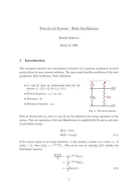
• |1〉 and |2〉 form an orthonormal basis for the
system i.e. 〈i|j〉 = δ ij for i, j = 1, 2 ;
∆
|2
• Photon frequency : ω = ω 0 + ∆ ;
• Detuning : ∆ ;
ω 0
ω
• Resonant frequency : ω 0 .
|1
Fig. 1: Two-level system.
With no driving field on, states |1〉 and |2〉 are (by definition) the energy eigenstates of the
system. They are eigenstates of the bare Hamiltonian (no applied field) Ĥ0 and as such have
a well defined energy:
Ĥ 0 |1〉 = 0 |1〉,
Ĥ 0 |2〉 = ω 0 |2〉 . (1.1)
If the system begins in an energy eigenstate, it only acquires a phase as it evolves i.e. if
|ψ(0)〉 = |i〉, then |ψ(t)〉 = e −iEit/ |i〉. This can be seen by showing |ψ(t)〉 satisfies the
Schrödinger equation:
d|ψ(t)〉
dt
= − i e−iE it/ E i |i〉 ,
= − i e−iE it/ Ĥ 0 |i〉 ,
= − i Ĥ0|ψ(t)〉 . (1.2)
1

Then, the probability of finding the system in the state |i〉 at any time is |〈i|ψ(t)〉| 2 =
|e −iE it/ | 2 = 1. It is for this reason the energy eigenstates are called stationary states.
Any two-level quantum state can be expressed as |ψ〉 = c 1 |1〉 + c 2 |2〉, where c 1 and c 2 are
complex state amplitudes and |c 1 | 2 + |c 2 | 2 = 1. Such a state can be represented by a twocomponent
vector;
( )
〈1|ψ〉
ψ = =
〈2|ψ〉
( )
c 1
. (1.3)
c 2
The probability of finding the system in state |i〉 is |〈i|ψ〉| 2 = |c i | 2 , (for i = 1, 2).
Any operator  can be represented by a 2 × 2 Hermitian matrix:
The bare Hamiltonian Ĥ0 is then represented as:
(
)
A =
〈1|Â|1〉 〈1|Â|2〉
〈2|Â|1〉 〈2|Â|2〉 . (1.4)
H 0 =
( )
0 0
. (1.5)
0 ω 0
What about the driving field? What does it do? It induces a dipole (electric or magnetic)
moment between the states |1〉 and |2〉. The electromagnetic field interacts with this dipole,
resulting in an oscillatory perturbation. This perturbation is represented by the operator:
(
)
0 Ω cos(ωt)
H int =
Ω ∗ , (1.6)
cos(ωt) 0
where Ω = µE 0 , with µ the induced dipole moment and E 0 is the amplitude of the electromagnetic
field. This interaction causes transitions between the two states. Why? Because
Ĥ|i〉 ≠ α|i〉, (i = 1, 2 and α a constant), so the states |1〉 and |2〉 are no longer stationary
states of the system. It is for this reason the two levels are said to be coupled by the applied
field. We will now look at the time evolution of the system starting in state |1〉 under the
application of an applied field.
2

2 Dynamics
2.1 Main Result : Rabi Oscillations
If the system begins at time t = 0 in state |1〉 and the field is applied, the state amplitudes
evolve such that;
( )
|c 1 (t)| 2 = Ω2
Ω 2 sin 2 ΩR t
,
R
2
( )
|c 2 (t)| 2 = ∆2
Ω 2 + Ω2
R
Ω 2 cos 2 ΩR t
R
2
Ω 2 R ≡ Ω 2 + ∆ 2 .
, (2.1)
This means that the probabilities to be in state |1〉 or |2〉 oscillate with the frequency Ω R
defined above, the total Rabi frequency. From this result, it is clear that states |1〉 and |2〉
are no longer stationary states of the system. It is remarkable that the dynamic behaviour
of the system is governed (at this point) by only two parameters. These parameters are the
coupling strength Ω (proportional to the electromagnetic field strength) and the detuning ∆
(how far the field is away from resonance).
The applied field still induces transitions between the two states for frequencies not exactly on
resonance (∆ ≠ 0). The solutions (2.1) show the contrast of the Rabi oscillations is dependent
upon the detuning. Only on resonance do the populations oscillate completely between zero
and unity. Away from resonance, the oscillations are faster but of lower amplitude. Also, for
a fixed detuning, the frequency of the oscillations can be varied by changing the strength of
the applied field. This is shown in the plots of Section 2.4.
2.2 Derivation of Rabi Oscillations
The result above is derived by solving the Schrödinger equation in the interaction picture.
This means that the time dependence of the Hamiltonian is removed by transforming to a
“rotating frame”.
Such a transformation is unitary (norm-preserving) and applied to the
total Hamiltonian H = H 0 + H int . To see how this works, first we rewrite the Hamiltonian
in the Schrödinger picture as (using equations (1.5) and (1.6)):
(
)
H = 2
0 Ω (e iωt + e −iωt )
Ω ∗ (e iωt + e −iωt ,
) 2ω 0
(2.2)
and define the following operator:
( )
0 0
H 1 = . (2.3)
0 ω
3

Then, the new Hamiltonian (in the interaction picture, or “rotating frame”) is given by the
following unitary transformation:
The matrix corresponding to the new Hamiltonian is:
Ĥ ′ = e iĤ1t/ (Ĥ − Ĥ1) e −iĤ1t/ . (2.4)
( ) (
) ( )
H ′ = 1 0
0 Ω (e iωt + e −iωt ) 1 0
2 0 e iωt Ω ∗ (e iωt + e −iωt ) 2(ω 0 − ω) 0 e −iωt ,
(
)
= 0 Ω (1 + e −i2ωt )
2 Ω ∗ (1 + e i2ωt . (2.5)
) −2∆
We then make the rotating wave approximation, which is to ignore terms that oscillate at
twice the driving frequency:
(
)
H ′ = 0 Ω
2 Ω ∗ . (2.6)
−2∆
To find the time evolution of the state amplitudes, the Schrödinger equation:
d|ψ〉
dt
= − i Ĥ′ |ψ〉 , (2.7)
is written in matrix form:
( ) (
) ( )
ċ 1 (t)
= − i 0 Ω c 1 (t)
ċ 2 (t) 2 Ω ∗
. (2.8)
−2∆ c 2 (t)
The Rabi frequency Ω can be made real by choosing the phase of the driving field to be zero.
Then the differential equations for the state amplitudes are:
ċ 1 (t) = − i 2 Ω c 2(t) ,
ċ 2 (t) = − i 2 Ω c 1(t) + i∆ c 2 (t) ,
c 1 (0) = 1 ,
c 2 (0) = 0 . (2.9)
The solution is:
( )
c 1 (t)
= e it∆ 2
c 2 (t)
⎛
(
⎝ cos ΩR t
2
)
− i ∆ Ω R
sin
)
−i Ω Ω R
sin
(
ΩR t
2
(
ΩR t
2
) ⎞
⎠ . (2.10)
4

2.3 State transfer and Superpositions
With the evolution of a system beginning in |1〉 known, consider driving the system on
resonance (∆ = 0) for a fixed length of time, before turning the driving field off. There are
two cases of interest, the π-pulse and the π 2
-pulse. In each case, we can use equation (2.10)
to find the resulting state.
A π-pulse corresponds to turning the field on at t = 0 and off at t = T π ≡ π/Ω. Then:
( )
0
ψ(T π ) = , (2.11)
−i
or equivalently:
|ψ(T π )〉 = −i|2〉 . (2.12)
Since an overall phase of a quantum state does not affect probabilities, this state is equivalent
to |2〉, and a π-pulse is said to transform |1〉 into |2〉.
A π 2 -pulse corresponds to turning the field on at t = 0 and off at t = T π
2
≡ π/(2Ω). Then:
( )
ψ(T π ) = √ 1 1
, (2.13)
2 2 −i
or equivalently:
|ψ(T π
2 )〉 = 1 √
2
(|1〉 − i|2〉) . (2.14)
This state is a special superposition, since the probability to be in either state |1〉 or |2〉 after
a π 2 -pulse is 1 2 . 5

2.4 Plots of Rabi Oscillations
Below are plots of the probabilities to be in state |1〉 or |2〉 (solid and dashed lines, respectively)
for various Rabi-frequencies and detunings (equations (2.1)):
1.0
⩵2Π,⩵0
1.0
⩵4Π,⩵0
0.8
0.8
probabilities
0.6
0.4
0.2
probabilities
0.6
0.4
0.2
0.0
0.0 0.5 1.0 1.5 2.0
time
0.0
0.0 0.5 1.0 1.5 2.0
time
1.0
⩵2Π,⩵2Π
1.0
⩵2Π,⩵4Π
0.8
0.8
probabilities
0.6
0.4
0.2
probabilities
0.6
0.4
0.2
0.0
0.0 0.5 1.0 1.5 2.0
time
0.0
0.0 0.5 1.0 1.5 2.0
time
6