The Euler Equation and the Gibbs-Duhem Equation - TUG
The Euler Equation and the Gibbs-Duhem Equation - TUG
The Euler Equation and the Gibbs-Duhem Equation - TUG

Create successful ePaper yourself
Turn your PDF publications into a flip-book with our unique Google optimized e-Paper software.
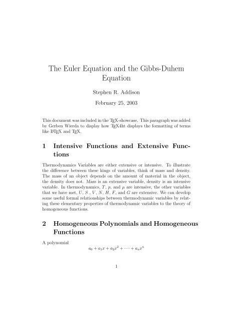
<strong>The</strong> <strong>Euler</strong> <strong>Equation</strong> <strong>and</strong> <strong>the</strong> <strong>Gibbs</strong>-<strong>Duhem</strong><br />
<strong>Equation</strong><br />
Stephen R. Addison<br />
February 25, 2003<br />
This document was included in <strong>the</strong> TEX-showcase. This paragraph was added<br />
by Gerben Wierda to display how TEX4ht displays <strong>the</strong> formatting of terms<br />
like L A TEX <strong>and</strong> TEX.<br />
1 Intensive Functions <strong>and</strong> Extensive Functions<br />
<strong>The</strong>rmodynamics Variables are ei<strong>the</strong>r extensive or intensive. To illustrate<br />
<strong>the</strong> difference between <strong>the</strong>se kings of variables, think of mass <strong>and</strong> density.<br />
<strong>The</strong> mass of an object depends on <strong>the</strong> amount of material in <strong>the</strong> object,<br />
<strong>the</strong> density does not. Mass is an extensive variable, density is an intensive<br />
variable. In <strong>the</strong>rmodynamics, T , p, <strong>and</strong> µ are intensive, <strong>the</strong> o<strong>the</strong>r variables<br />
that we have met, U, S , V , N, H, F , <strong>and</strong> G are extensive. We can develop<br />
some useful formal relationships between <strong>the</strong>rmodynamic variables by relating<br />
<strong>the</strong>se elementary properties of <strong>the</strong>rmodynamic variables to <strong>the</strong> <strong>the</strong>ory of<br />
homogeneous functions.<br />
2 Homogeneous Polynomials <strong>and</strong> Homogeneous<br />
Functions<br />
A polynomial<br />
a 0 + a 1 x + a 2 x 2 + · · · + a n x n<br />
1
is of degree n if a n ≠ 0. A polynomial in more than one variable is said to<br />
be homogeneous if all its terms are of <strong>the</strong> same degree, thus, <strong>the</strong> polynomial<br />
in two variables<br />
x 2 + 5xy + 13y 2<br />
is homogeneous of degree two.<br />
We can extend this idea to functions, if for arbitrary λ<br />
it can be shown that<br />
f(λx) = g(λ)f(x)<br />
f(λx) = λ n f(x)<br />
a function for which this holds is said to be homogeneous of degree n in <strong>the</strong><br />
variable x. For reasons that will soon become obvious λ is called <strong>the</strong> scaling<br />
function. Intensive functions are homogeneous of degree zero, extensive<br />
functions are homogeneous of degree one.<br />
2.1 Homogeneous Functions <strong>and</strong> Entropy<br />
Consider<br />
S = S(U, V, n),<br />
this function is homogeneous of degree one in <strong>the</strong> variables U, V , <strong>and</strong> n,<br />
where n is <strong>the</strong> number of moles. Using <strong>the</strong> ideas developed above about<br />
homogeneous functions, it is obvious that we can write:<br />
S(λU, λV, λn) = λ 1 S(U, V, n),<br />
where λ is, as usual, arbitrary. We can gain some insight into <strong>the</strong> properties<br />
of such functions by choosing a particular value for λ. In this case we<br />
will choose λ = 1 so that our equation becomes<br />
n<br />
( U<br />
S<br />
n , V )<br />
n , 1<br />
= 1 S(U, V, n)<br />
n<br />
Now, we can define U = u, V = v <strong>and</strong> S(u, v, 1) = s(u, v), <strong>the</strong> internal energy,<br />
n n<br />
volume <strong>and</strong> entropy per mole respectively. Thus <strong>the</strong> equation becomes<br />
ns(u, v) = S(U, V, n),<br />
<strong>and</strong> <strong>the</strong> reason for <strong>the</strong> term scaling function becomes obvious.<br />
2
3 <strong>The</strong> <strong>Euler</strong> <strong>Equation</strong><br />
Consider<br />
U(λS, λV, λn) = λU(S, V, n)<br />
differentiating with respect to λ (<strong>and</strong> changing sides of <strong>the</strong> equation) this<br />
becomes<br />
( )<br />
( )<br />
( )<br />
∂U ∂(λS) ∂U<br />
U(S, V, n) =<br />
∂(λS) ∂λ + ∂(λV ) ∂U<br />
∂(λV ) ∂λ + ∂(λn)<br />
∂(λn) ∂λ<br />
V,n<br />
S,n<br />
S,V<br />
which simplifies to<br />
U(S, V, n) =<br />
( ) ( ) ( )<br />
∂U<br />
∂U<br />
∂U<br />
S +<br />
V +<br />
n.<br />
∂(λS) ∂(λV ) ∂(λn)<br />
V,n<br />
S,n<br />
S,V<br />
Recalling that λ is arbitrary, we now choose λ = 1, resulting in<br />
( ) ( ) ( )<br />
∂U ∂U ∂U<br />
U(S, V, n) = S + V + n,<br />
∂S ∂V<br />
∂n<br />
V,n<br />
S,n<br />
S,V<br />
<strong>and</strong> recognizing that <strong>the</strong> partial derivatives in this equations are now just<br />
<strong>the</strong> definitions of <strong>the</strong> extensive variables T , p, <strong>and</strong> n, we can rewrite this as<br />
U = T S − pV + µn.<br />
This equation, arrived at by purely formal manipulations, is <strong>the</strong> <strong>Euler</strong> equation,<br />
an equation that relates seven <strong>the</strong>rmodynamic variables.<br />
3.1 <strong>The</strong> relationship between G <strong>and</strong> µ<br />
Starting from<br />
<strong>and</strong> using<br />
we have<br />
U = T S − pV + µn.<br />
G = U + pV − T S<br />
G = T S − pV + µn + pV − T S = µn.<br />
So for a one component system G = µn, for a j-component system, <strong>the</strong> <strong>Euler</strong><br />
equation is<br />
j∑<br />
U = T S − pV + µ i n i<br />
3<br />
i=1
<strong>and</strong> so for a j-component system<br />
j∑<br />
G = µ i n i<br />
i=1<br />
4 <strong>The</strong> <strong>Gibbs</strong>-<strong>Duhem</strong> <strong>Equation</strong><br />
<strong>The</strong> energy form of <strong>the</strong> <strong>Euler</strong> equation<br />
expressed in differentials is<br />
U = T S − pV + µn<br />
dU = d(T S) − d(pV ) + d(µn) = T dS + SdT − pdV − V dp + µdn + ndµ<br />
but, we know that<br />
<strong>and</strong> so we find<br />
dU = T dS − pdV + µdn<br />
0 = SdT − V dp + ndµ.<br />
This is <strong>the</strong> <strong>Gibbs</strong>-<strong>Duhem</strong> equation. It shows that three intensive variables<br />
are not independent – if we know two of <strong>the</strong>m, <strong>the</strong> value of <strong>the</strong> third can be<br />
determined from <strong>the</strong> <strong>Gibbs</strong>-<strong>Duhem</strong> equation.<br />
4