Template for the Preparation of Abstract

XXI International Symposium, Research-Education-Technology 

Gdansk, May 23 th – 24 th , 2013 

Experimental and numerical investigation of thin liquid layers at curved solid edges 

Oliver Sommer, Daniel Moller, Günter Wozniak 

Chemnitz University of Technology, Faculty of Mechanical Engineering, 

Institute of Mechanics and Thermodynamics, Chair of Fluid Mechanics 

Chemnitz, D-09107, Germany 

oliver.sommer@mb.tu-chemnitz.de, daniel.moller@mb.tu-chemnitz.de, guenter.wozniak@mb.tu-chemnitz.de 

Keywords: laser induced fluorescence, computational fluid dynamics, thin liquid layer, curved surface, thickness distribution 

Abstract 

The knowledge of the behavior of thin liquid layers on 

solid surfaces is of fundamental interest as far as basic 

research or applications like technical coating or lubrication 

processes are concerned. The subject is currently getting 

more important, particularly due to the increasing 

requirements of thin liquid layer functionalities. 

We therefore studied the development of the liquid 

layer thickness distribution field as well as the film 

disturbance propagation on a plane solid surface in the 

vicinity of a curved solid edge experimentally and 

numerically using LIF (Laser-induced Fluorescence) and 

CFD (Computational Fluid Dynamics), respectively. 

The investigation focusses on the influence of the 

initial layer thickness and solid surface curvature as well as 

liquid properties like viscosity and surface tension on the 

film behavior, especially close to solid edges. Experimental 

and numerical results are shown pointing out relevant 

quantities for disturbance propagation and validation. 

1 Introduction 

A fundamental problem of coating is the adhesion 

between the liquid (later on the solidified liquid) and solid 

surface, facilitating through these physical phenomena the 

bonding of the coating on the substrate. Another problem is 

leveling and sagging, caused by gravity and in dependence 

on the viscosity, particularly the rebounding viscosity under 

low shearing conditions, after having applied high shearing 

conditions through applications like painting or atomization 

earlier. Our investigation also focusses on the liquid state, 

however the disturbance effects on the justified 

homogeneous liquid layer thickness applied on plane solid 

surfaces in the vicinity of curved solids edges. This 

phenomenon is known as edge/ corner thinning in coating 

applications (Meichsner et al. 2003, Mischke 2007), 

although the statements and assumptions are focused on the 

curved solid surface area, which is losing liquid thickness. 

Our investigation is focused on the disturbance of the 

initial homogeneous thin liquid layer on the plane solid 

surface area at a curved solid edge (see fig. 2) and the 

influence on the curved solid edge parts, too. For these 

intensions we present and describe our experimental and 

numerical setup. The results of both approaches will be 

compared by introducing characteristic variables of the 

disturbance description. With this study we want to deliver a 

contribution to the understanding of the underlying physics 

of the edge thinning effect and the disturbance as well as to 

give some information regarding technical applications. 

2 Theoretical background 

Imagine a homogeneous thin liquid layer at a curved 

solid edge. Four acting forces are expected in this situation. 

These are basically the capillary force due to the surface 

tension, inertia and viscous force due to liquid flow and 

intermolecular interaction, respectively and the gravity force. 

The capillary force develops from the capillary pressure, 

which is described by Young-Laplace’s equation for the 

pressure jump on a free liquid surface: 

1 1 

p 

 

. (1) 

R1 R 2 

Since in our case the second radius of curvature goes 

to infinity, equation (1) leads to 

 

p . (2) 

R 

The pressure jump is here the hydrostatic pressure 

p = g h, representing the gravity and can be seen as a 

counterpart to the capillary pressure. Hence, it is possible to 

yield the dimensionless Bond-number Bo, which is defined 

as hydrostatic pressure in relation to the capillary pressure: 

g h R 

Bo . (3) 

 

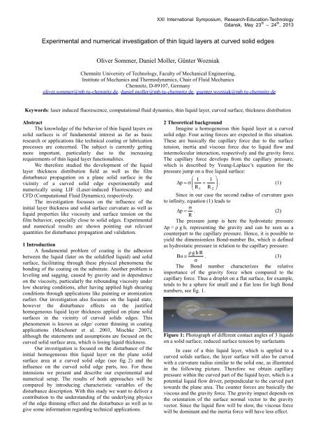
The Bond number characterizes the relative 

importance of the gravity force when compared to the 

capillary force. Thus a droplet on a flat surface, for example, 

tends to be a sphere for small and a flat lens for high Bond 

numbers, see fig. 1. 

Figure 1: Photograph of different contact angles of 3 liquids 

on a solid surface; reduced surface tension by surfactants 

In case of a thin liquid layer, which is applied to a 

curved solids surface, the layer surface will also be curved 

with a curvature radius similar to the solid one, as illustrated 

in the following picture. Therefore we obtain capillary 

pressure within the curved part of the liquid layer, which is a 

potential liquid flow driver, perpendicular to the curved part 

towards the plane area. The counter forces are basically the 

viscous and the gravity force. The gravity impact depends on 

the orientation of the surface normal vector to the gravity 

vector. Since the liquid flow will be slow, the viscous force 

will be dominant and the inertia force will have less effect.



Figure 2: Illustration of the edge/ corner thinning effect and 

the disturbance effect of the liquid layer 

Once a steady state is reached, a disturbance of the 

former homogeneous liquid layer in form of a hump will be 

visible. It develops parallel to the curved solid edge within 

the plane solid surface part. 

3 Experimental setup 

For the experiments on the liquid layer thickness 

distribution the so-called Laser-induced Fluorescence 

technique LIF was used, which is applied usually for 

measurement and propagation of liquid-liquid or sometimes 

of liquid-gas mixing problems as well as problems in 

microbiology, microfluidics and in fluid mechanic heat and 

mass transfer problems (Glawdel el al. (2008) and Petracci 

et al. (2006)). In this experimental investigation the general 

idea of measuring liquid thickness using LIF, allowing 

non-invasive and therefore non-destructive detections, is 

similar to investigations of Ausner et al. (2005) and Ausner 

(2006) but in much smaller liquid thickness dimensions and 

in different experimental setups. 

The need of fluorescing substances, which can be 

mixed into the applied liquid without changing the liquid 

properties, is mandatory as well as an exciting light source 

and a camera device, equipped with optical filters for signal 

detection. The applied fluorescence substance was mixed 

into the liquid with a mass weight ratio of about 1:10,000, 

resulting in negligible changes in liquid properties like 

density, viscosity and surface tension. The use of suitable 

optical filters in front of the camera device is necessary to 

avoid detection of disturbing light intensity. In our case we 

used a so-called band-pass filter, which permits a light 

transparency close to 1.0 in the relevant wavelength, while 

blocking all other wavelengths. The exciting light source 

was a diode-laser with an emitting wavelength of 

= 532 nm and a constant optical power output of 

P = 40 mW. Equipped with a special optical lens (a so-called 

Powell lens), it was possible to achieve an anti-Gaussian 

spaced line profile of the laser beam within objective 

distances of 200 mm ≤ l ≤ ∞. 

The typical experimental setup of the above mentioned 

light source, camera device and solid substrate is shown as 

schematic in fig. 3. The orthogonal arrangement of the light 

source and the camera device to the solid substrate is well 

visible as well as the homogenous distributed laser line 

profile and the band-pass filter in front of the camera device. 

For our needs of an objective distance to solid/ liquid surface 

l ≥ 0.5 m (space for coating application), we used an 

objective of f = 80 mm focal length in combination with 

intermediate rings (50 mm) and yield a photograph (range of 

interest, ROI) of about 58.5 mm x 10.5 mm. The camera 

device was a b/ w Basler Scout type with a maximum spatial 

resolution of 1392 Pixel x 1040 Pixel and 12 bit intensity 

resolution. The maximum frame grabbing speed was about 

17 fps. 

Figure 3: Schematic of the experimental arrangement 

For camera controlling a Labview program was written 

to apply typical camera and acquisition parameters including 

the region of interest (ROI) and the rate of visual recording 

(fps). A second Labview program was used for picture post 

processing. Figure 4 shows a typically photograph of one 

parameter setup of the liquid layer distribution using the LIF 

technique. A good visibility has been identified due to the 

higher emitted intensity of the liquid layer disturbance at the 

solid surface curvature on the left side, while the rest of the 

emitted line has about the same intensity. 

Figure 4: Photograph of a typical liquid layer thickness 

distribution at curved solid surface with LIF technique 

The corresponding liquid layer thickness distribution, 

which is generated by our post processing program, is 

measured in dimensionless intensity units and the position is 

given in Pixel, see fig. 5. 

Figure 5: Experimental result of a typical liquid layer 

intensity distribution at a curved solid surface 

This figure also shows the respective variables for the 

disturbance description of the homogenous film at the 

curved solid surface, namely the bandwidth x, the 

maximum emitted light intensity I max and its position x max . 

The averaged intensity I avg at a distance of the solid surface 

curvature is illustrated, too. The ratio of justified liquid layer 

thickness, which is calculated by multiplication of the 

measured solidified thickness with the factor 2, and the 

averaged intensity yields in an intensity-liquid thickness 

scaling factor b. In the same manner the geometric scaling 

factor a is obtained, here by the ratio of measured distance in

length unit to the counted number of Pixel. Using these two 

scaling factors, the maximum liquid layer thickness and its 

position are obtained in length units, see fig. 6. 



The liquid layer maximum thickness s max and its 

normalized position to the substrate beginning x max are yield 

by a polynomial fit of the intensity values within the 

bandwidth array mentioned earlier, and a following search of 

the peak value. Tracked over the time the normalized 

position x max becomes a characteristic velocity of the rise. 

With the bandwidth-time plot in mind, the plots of the 

maximum liquid layer thickness s max , the justified liquid 

layer thickness s avg as well as the ratio s* = s max / s avg of both 

give a good picture for the development of the disturbance 

of the thin liquid layer at solid curved edges in space and 

time. 

Figure 6: Experimental result of a typical liquid layer 

thickness distribution at a curved solid surface 

The three important variables mentioned before, are 

tracked over the time until no more change was visible, see 

fig. 7-9. In each diagram there is a black vertical line, 

representing the end of the coating application, which means 

that at this time, and further on, the disturbance of the 

homogeneous film could develop without external acting 

forces of the atomizer. The bandwidth x is built through an 

array length, which contains the intensity (thickness) values, 

which are 105 % or higher than the averaged values from the 

non-influenced area of the liquid layer, see fig. 5. 

Figure 7: Liquid layer bandwidth x tracked over the time t 

Figure 8: Position of the maximum liquid layer 

thickness x max tracked over the time t 

Figure 9: Maximum liquid layer thickness s max (blue), 

justified liquid layer thickness s avg (red) and relative max. 

liquid layer thickness s* (green) at a solid surface edge 

tracked over time t 

Preconceiving a ratio of bandwidth and maximum 

liquid layer thickness, this value will represent the surface 

normal gradient, which will distinguish between good 

visible and not so conspicuous disturbances of the 

homogeneous liquid layer. Depending on the parameter 

configuration the disturbance rise comes to rest after about 

30 to 40 seconds. Curve fitting has been applied to each 

variable (fig. 7-9), to yield values describing the final steady 

state of the disturbance of the thin liquid layer at curved 

solid edges. 

4 Numerical setup 

For the numerical approach we used a commercial 

available CFD code, termed STAR-CCM + from the 

company cd-adapco. This software contains different 

methods for modeling multiphase flows. Since we are 

interested in the resolving and tracking of the liquid-gas 

interface, i.e. the liquid surface curvature and thus the 

capillary pressure, the use of the Eulerian approach based 

Volume of Fluid Method (VOF) has been applied. This 

method uses the level-set method by Brackbill et al. (1992) 

and is capable to simulate and to display the liquid surface 

of a liquid-gas fluid arrangement, e.g. the liquid depth or 

wave height in typical marine applications. 

Our interest lies in the liquid depth, particularly in the 

liquid layer thickness on a curved solid substrate in 

connection with capillary pressure and corresponding 

capillary forces driven effects on the homogenous justified 

film. Beside the VOF model, other physical models were 

applied like gravity, laminar flow and transient time regime. 

In a similar manner liquid and gas properties (see table 1), 

boundary and initial conditions were set.

Table 1: typical fluid property configuration 

liquid 

gas 

= 1,020 kg/ m 3 = 1.184 kg/ m 3 

(t) = 0.2 Pa s + 0.02 Pa ∙ t = 0.018 mPa s 

= 28.0 mN/ m 

The following two pictures show a typical simulation 

at the beginning and the result after 20 seconds. Clearly 

visible, a homogeneous thin liquid layer of justified 

thickness and surface curvatures exists. The liquid layer 

thickness is displayed as scalar field on the liquid surface as 

a blue to red scale, where blue indicates small values and red 

bigger thicknesses. With the intension of reducing 

computational effort, two different solid surface curvatures 

were applied. On the left side we always found a bigger 

curvature radius than on the right side and the plane area 

situated between the two curved parts was built large enough 

to avoid overlapping of both developing humps. 



The bandwidth x and the maximum liquid layer 

thickness s max and its position x max were evaluated and 

plotted over the time, likewise in the experimental post 

processing. 

An effective simulation means an optimal spatial and 

temporal resolution in combination with the time effort of 

one simulation including post processing. Thus, verification 

simulations with different resolutions of the numeric mesh 

and transient time steps were performed (fig. 13). It turned 

out that a mesh with about 1 million elements in 

combination with a transient time step of t = 0.001 s was 

the best compromise between numeric accuracy and real 

time effort. Here a local spatial resolution of 1 % to 5 % of 

the quarter circumference, built by the solid surface 

curvature, was applied in combination with an equidistantly 

grown boundary layer mesh, which allowed a liquid 

thickness resolution of about 2.0 µm. 

Figure 10: Initial liquid layer thickness distribution at t = 0 s 

Figure 13: Numerical verification of the model using 

different spatial and temporal resolutions 

The following three pictures (fig. 14-16) show the time 

plots of the bandwidth x, the maximum liquid layer 

thickness s max and its position x max at the plane solid surface, 

likewise in the experiment. 

Figure 11: Liquid layer thickness distribution at t = 20 s 

For post processing, the liquid layer thickness 

distribution in the middle of the substrate’s height is 

extracted as a line probe every second and plotted over the 

plane area position, see fig. 12. 

Figure 14: Liquid layer bandwidth x versus the time t 

Figure 12: Numerical result of a typical liquid layer 

thickness distribution at curved solid surfaces at t = 20 s 

The bandwidth x decreases with time in the same 

manner as in the experiments. This also is the case for the 

maximum liquid layer thickness position time plot as well as 

the maximum liquid layer thickness sequence. A curve 

fitting was applied to the numerically achieved 

bandwidth x, the position x max and height of the maximum 

liquid layer thickness s max to get the steady state values of 

the problem.



the numerical time, which is identical to the application 

duration of the experimental application. 

Figure 15: Position of the maximum liquid layer thickness 

x max tracked over the time t 

Figure 17: Comparison of experimental (blue dots) and 

numerical results (red line); bandwidth x versus time t 

Figure 16: Maximum liquid layer thickness s max 

(blue: r C = 3.0 mm, red: r C = 2.0 mm) close to the solid 

surface curvature and relative max. liquid layer thickness s* 

(green: r C , violet: r C ) tracked as a function of time t 

Since the computational resources were limited, the 

simulation time ended with 20 seconds in each simulation 

run. This duration was adequate for a good comparison of 

the experimental and numerical results, because the 

diagrams 14-16 show that there were no more drastic 

changes expected. 

5 Results and discussion 

The following 3 diagrams illustrate the liquid layer 

bandwidth x, the maximum liquid layer thickness 

position x max and the maximum liquid layer thickness s max 

over the time t of one experimental (blue dots) and one 

numerical result (red line), which were performed with an 

identical parameter setup. It is clearly visible, that they fit 

each other quite well. Very small deviations are only visible 

between the experimental dots and the numerical lines 

within the 12 th to the 30 th second. This can be explained by 

the small errors which occur in both investigation 

approaches through the compromises, which had to be 

applied, facilitating this investigation in general. 

Nevertheless the time dependent functions of the chosen 

variables for the disturbance description are very similar and 

therefore the steady state values are very close to equality. 

The numerical curves always begin later with time 

than the experimental ones. This is due to the ideal initial 

conditions in the numerical simulation. Here we could set a 

homogeneous distributed liquid film of desired thickness at 

the beginning, while in the experiments we had to apply it 

first by a suitable application. Thus we set an offset-time to 

Figure 18: Comparison of experimental and numerical 

results; maximum thickness position x max versus time t 

Figure 19: Comparison of experimental (blue dots) and 

numerical results (red line); maximum liquid layer thickness 

s max versus time t 

These diagrams also show that our chosen total 

simulation time, which is smaller than the experimental time, 

is well suitable to predict the liquid layer thickness 

distribution and therefore the disturbance of thin liquid 

layers at curved solid edges. Furthermore, the simulation 

shows the liquid layer thickness distribution on the curved 

part of a solid, too. Thus a prediction of the edge/ corner 

thinning effect would also be possible, fig. 20.



T. Glawdel et al., Photobleaching absorbed Rhodamine B to 

improve temperature measurements in PDMS microchannels. 

Lab on Chip, Vol. 9, 171-174 (2009) 

A. Petracci, R. Delfos, J. Westerweel, Combined PIV/LIF 

measurements in a Rayleight-Bénard convection cell. 13 th 

Int. Symp. on Applications of Laser Techniques to Fluid 

Mechanics, Lisbon, Portugal (2006) 

Figure 20: Liquid layer thickness distribution on a curved 

solid surface at t = 20.0 s 

6 Concluding remarks and outlook 

In this investigation we studied the possibility of an 

experimental measurement and a numerical simulation of 

the transient development of the disturbance of a thin liquid 

layer at a curved solid edge and in the steady state. For this 

we developed a suitable experimental setup with a 

self-written program code for semi-automatic post 

processing. A suitable numerical approach was established, 

too. We identified convenient variables for the description of 

the disturbance development and for an interpretation in 

view of technical applications. The experimental and 

numerical results fit each other very well, so that predictions 

of the liquid layer thickness distributions on solid surfaces 

are possible. Furthermore the numerical approach is capable 

to give results describing the edge thinning effect. 

Future investigations as well as already on-going 

studies are focused on the influences of the dependencies of 

typical technical parameters and liquid properties. However 

the normal orientation vector of the substrate, material and 

roughness of the substrate as well as other coating 

applications will be taken into account, too. 

I. Ausner, A. Hoffmann, J.-U. Repke and G. Wozny, 

Experimentelle und numerische Untersuchungen 

mehrphasiger Filmströmungen. Chemie Ingenieur Technik, 

Vol. 77, No. 6, 735-741 (2005) 

I. Ausner, Experimentelle Untersuchungen mehrphasiger 

Filmströmungen. Dissertation, TU Berlin (2006) 

H. Du et al., PhotochemCAD: A computer-aided design and 

research tool in photochemistry. Photochem. Photobiol. Vol. 

68 (2), 141-142 (1998) 

J.U. Brackbill, D.B. Kothe and C. Zemach, A Continuum 

Method for Modeling Surface Tension, Journal of 

Computational Physics, Vol. 100, 335-354 (1992) 

T.G. Mezger, Das Rheologie Handbuch, Vincentz Network, 

Hannover (2010) 

Nomenclature 

symbol description unit 

a geometric scale factor [mm/ px] 

b intensity-liquid thickness scale factor [µm/ -] 

I avg averaged emitted light intensity [-] 

I max maximum emitted light intensity [-] 

r C solid surface curvature radius [mm] 

r l liquid surface curvature radius [mm] 

s avg justified liquid layer thickness [µm] 

s max maximum liquid layer thickness [µm] 

s* relative maximum liquid layer thickness [%] 

t time [s] 

x max maximum liquid layer thickness position [mm] 

x liquid layer disturbance bandwidth [mm] 

 

viscosity [Pa s] 

density [kg/ m 3 ] 

surface tension [mN/ m] 

References 

G. Meichsner, T.G. Mezger, J. Schröder, Lackeigenschaften 

messen und steuern. Coatings Compendien, Vincentz 

Network, Hannover (2003) 

P. Mischke, Filmbildung. Filmbildung in modernen 

Lacksystemen. Vincentz Network, Hannover (2007)

Template for the Preparation of Abstract

Create successful ePaper yourself

Delete template?

Save as template?