bubble pump modeling for solar hot water heater system design

A L
1
[15]
A 2
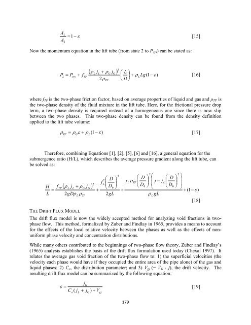
Now the momentum equation in the lift tube (from state 2 to P sys ) can be stated as:
2
TP
2
L
jL
G
jG
L
P Psys fTP
LLg(1
)
[16]
2
D
where f TP is the two-phase friction factor, based on average properties of liquid and gas and ρ TP is
the two-phase density of the fluid mixture in the lift tube. Here, for the frictional pressure drop
term, a two-phase density is required instead of a homogeneous one since there is now slip
between the two phases. This two-phase density can be found from the density definition
applied to the lift tube volume:
TP G
L( 1
)
[17]
Therefore, combining Equations [1], [2], [5], [6] and [16], a general equation for the
submergence ratio (H/L), which describes the average pressure gradient along the lift tube, can
be solved as:
H
L
f
TP
j
L
L
j
2gD
L
G
TP
G
2
j
2
L
D
D0
2gL
4
j
L
TP
D
D
0
2
j
gL
L
j
L
D
D
0
2
(1
)
[18]
THE DRIFT FLUX MODEL
The drift flux model is now the widely accepted method for analyzing void fractions in twophase
flow. This method, formalized by Zuber and Findlay in 1965, provides a means to account
for the effects of the local relative velocity between the phases as well as the effects of nonuniform
phase velocity and concentration distributions.
While many others contributed to the beginnings of two-phase flow theory, Zuber and Findlay’s
(1965) analysis establishes the basis of the drift flux formulation used today (Chexal 1997). It
relates the average gas void fraction of the two-phase flow to: 1) the superficial velocities (the
velocity each phase would have if they occupied the entire area of the pipe alone) of the gas and
liquid phases; 2) C o , the distribution parameter; and 3) V gj (= V G - j), the drift velocity. The
resulting drift flux model can be summarized by the following equation:
G
[19]
C ( j
o
L
j
j
G
) V
gj
179