bubble pump modeling for solar hot water heater system design
bubble pump modeling for solar hot water heater system design
bubble pump modeling for solar hot water heater system design

You also want an ePaper? Increase the reach of your titles
YUMPU automatically turns print PDFs into web optimized ePapers that Google loves.
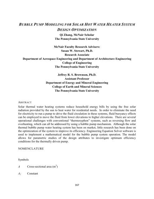
BUBBLE PUMP MODELING FOR SOLAR HOT WATER HEATER SYSTEM<br />
DESIGN OPTIMIZATION<br />
Qi Zhang, McNair Scholar<br />
The Pennsylvania State University<br />
McNair Faculty Research Advisers:<br />
Susan W. Stewart, Ph.D.<br />
Research Associate<br />
Department of Aerospace Engineering and Department of Architecture Engineering<br />
College of Engineering<br />
The Pennsylvania State University<br />
Jeffrey R. S. Brownson, Ph.D.<br />
Assistant Professor<br />
Department of Energy and Mineral Engineering<br />
College of Earth and Mineral Sciences<br />
The Pennsylvania State University<br />
ABSTRACT<br />
Solar thermal <strong>water</strong> heating <strong>system</strong>s reduce household energy bills by using the free <strong>solar</strong><br />
radiation provided by the sun to heat <strong>water</strong> <strong>for</strong> residential needs. In order to eliminate the need<br />
<strong>for</strong> electricity to run a <strong>pump</strong> to drive the fluid circulation in these <strong>system</strong>s, fluid buoyancy effects<br />
can be employed to move the fluid from lower elevations to higher elevations. There are several<br />
operational challenges with conventional “thermosyphon” <strong>system</strong>s, such as reversing flow and<br />
overheating, which can all be addressed by using a <strong>bubble</strong> <strong>pump</strong> mechanism. Although the <strong>solar</strong><br />
thermal <strong>bubble</strong> <strong>pump</strong> <strong>water</strong> heating <strong>system</strong> has been on market, little research has been done on<br />
the optimization of the <strong>system</strong> to improve its efficiency. Engineering Equation Solver software is<br />
used to implement a mathematical model <strong>for</strong> the <strong>bubble</strong> <strong>pump</strong> <strong>system</strong> operation. The model<br />
allows <strong>for</strong> parametric studies of the <strong>design</strong> attributes to investigate optimum efficiency<br />
conditions <strong>for</strong> the thermally driven <strong>pump</strong>.<br />
NOMENCLATURE<br />
Symbols<br />
A Cross-sectional area (m 2 )<br />
A 1<br />
Constant<br />
167
Bo<br />
B 1<br />
Bond Number<br />
Constant<br />
C Constant (with subscripts 1-8)<br />
C o<br />
C n<br />
Distribution parameter<br />
Constants in Chexal-Lellouche Void Model (n = 1,2, …8)<br />
COP Coefficient of Per<strong>for</strong>mance<br />
D<br />
D o<br />
D 2<br />
f<br />
f ’<br />
Diameter of lift tube (m)<br />
Diameter of entrance tube (m)<br />
Reference diameter (m)<br />
Friction factor<br />
Fanning friction factor<br />
g Acceleration of gravity (m/s 2 )<br />
H<br />
j<br />
K<br />
K o<br />
L<br />
L o<br />
L C<br />
m<br />
Height of Generator liquid level (m)<br />
Superficial velocity (m/s)<br />
Experimental friction relationship<br />
Correlating fitting parameter<br />
Length of lift tube (m)<br />
Length of entrance tube (m)<br />
Chexal-Lellouche fluid parameter<br />
Constant (different drift flux analysis than in slug/churn transition analysis)<br />
.<br />
m<br />
n<br />
N f<br />
Mass flow rate (kg/s)<br />
Constant<br />
Viscous effects parameter<br />
168
P<br />
Q<br />
Pressure (bars)<br />
Volumetric flow rate (m 3 /s)<br />
.<br />
Q<br />
Heat transfer rate (W)<br />
r<br />
Re<br />
S<br />
T<br />
V<br />
x<br />
Y<br />
Correlating fitting parameter<br />
Reynolds number<br />
Slip between phases of two-phase flow<br />
Temperature (K)<br />
Velocity (m/s)<br />
Quality<br />
Mole fractions<br />
Greek characters<br />
<br />
R<br />
Void fraction<br />
Pipe roughness (m)<br />
Density (kg/m 3 )<br />
<br />
<br />
<br />
Fluid viscosity (kg/m-s)<br />
Surface tension (N/m)<br />
Surface tension number<br />
.<br />
Volumetric Flow Rate (m 3 /s)<br />
Subscripts<br />
0 State 0 (in governing equations)<br />
1 State 1 (in governing equations)<br />
2 State 2 (in governing equations)<br />
a<br />
Ammonia<br />
169
BP<br />
G<br />
gj<br />
h<br />
L<br />
m<br />
TP<br />
v<br />
w<br />
Bubble <strong>pump</strong><br />
Gas<br />
Drift<br />
Homogeneous conditions (in two-phase flow)<br />
Liquid<br />
Mixture<br />
Two-phase<br />
Vertical<br />
Water<br />
Superscripts<br />
* non-dimensionalized<br />
NTRODUCTION<br />
Renewable energy technologies, such as wind and <strong>solar</strong> power, are being widely studied by<br />
researchers today as many countries are trying to reduce their dependence on non-renewable<br />
energy sources (i.e. fossil fuels). Massive use of conventional, non-renewable resources produces<br />
greenhouse gases which contribute significantly to climate change. Renewable energy sources,<br />
such as <strong>solar</strong> and wind energy, on the other hand, do not produce greenhouse gases. They are<br />
sustainable and free of cost.<br />
According to the World Watch Institute (WWI, 2011), “The United States, with less than 5 % of<br />
the global population, uses about a quarter of the world’s fossil fuel resources—burning up<br />
nearly 25 % of the coal, 26 % of the oil, and 27 % of the world’s natural gas.” In 2009, buildings<br />
consumed 72% of electricity and 55% natural gas of total consumption in the US. Water heating<br />
<strong>for</strong> buildings accounted <strong>for</strong> about 4% of the total energy used in 2009.<br />
170
Figure 1: US Energy Consumption by Sectors<br />
Solar thermal <strong>water</strong> heating (STWH) <strong>system</strong>s are both cost efficient and energy efficient. The<br />
STWH <strong>system</strong>s are most suitable <strong>for</strong> places with <strong>hot</strong> climates and direct sunlight, but can also<br />
work quite well in colder climates found throughout the United States. Different <strong>design</strong>s of the<br />
STWH <strong>system</strong>s have overcome the challenges such as freezing, and overheating. Most STWH<br />
<strong>system</strong>s have a flat plate <strong>solar</strong> collector tilted towards the south on the roof of the residence as<br />
shown in Figure 2. Flat plate <strong>solar</strong> panels consist of four parts: A transparent cover which allows<br />
minimal convection and radiation heat loss, dark color flat plate absorber <strong>for</strong> maximum heat<br />
absorption, pipes which carries heat transfer fluid that remove heat from the absorber, and a heat<br />
insulated back to prevent conduction heat loss. Within this collector, there is a network of black<br />
tube inside which flows <strong>water</strong> or some other fluid. The fluid in the tube enters the panel<br />
relatively cold and is heated as it flows through the panel as the black exterior of the tubes<br />
absorbs the heat from the sun. The heat transfer fluid and the materials selected <strong>for</strong> the tubes are<br />
important parameters <strong>for</strong> the <strong>system</strong> to withstand drastic temperature differences of freezing and<br />
overheating. If the fluid is <strong>water</strong>, then it goes right into a <strong>hot</strong> <strong>water</strong> storage tank. If another<br />
working fluid is used, the heat is then transferred from the working fluid to the <strong>water</strong> in the <strong>hot</strong><br />
<strong>water</strong> tank via a heat exchanger in the tank.<br />
171
Figure 2: Simple Schematic of a STWH 1<br />
Two of the most common STWH <strong>system</strong> types are passive and active <strong>system</strong>s. The fluid in a<br />
passive <strong>system</strong> is driven by natural convection, whereas in active <strong>system</strong>s, the fluid is moved via<br />
a <strong>pump</strong>. Active <strong>system</strong>s would be more reliable; however, they require another <strong>for</strong>m of energy<br />
input other than <strong>solar</strong> energy to run the <strong>pump</strong>s inside the <strong>system</strong>s. Thus, passive <strong>system</strong>s are<br />
preferred <strong>for</strong> economic purposes, but they have their own set of technical challenges.<br />
One of the most favorable passive <strong>system</strong>s is a thermosyphon STWH <strong>system</strong>, shown in Figure 3.<br />
A thermosyphon is an open loop <strong>system</strong> that can only be used <strong>for</strong> nonfreezing climates. The<br />
simple <strong>design</strong> of the thermosyphon <strong>system</strong> is economically efficient. Theoretically, in a<br />
thermosyphon <strong>system</strong>, the tank has to be above the <strong>solar</strong> panel. Using gravity, the cold <strong>water</strong><br />
from the tank flows downward and enters the tube beneath the panel, and gets heated up inside<br />
the tube. During this process, similar to a <strong>hot</strong> air balloon, the less dense <strong>hot</strong> <strong>water</strong> is buoyant and<br />
thus floats to the top of the tube and slowly reaches the top of the tank. Then, more cold <strong>water</strong><br />
would drain down from the tank and get heated up. The process continues on until the <strong>water</strong> of<br />
the tank reaches thermal equilibrium. Although the <strong>system</strong> seems ideal, there are problems such<br />
as overheating and freezing. Furthermore, the temperature differences of the tank from sunrise to<br />
sunset will always be positive; there<strong>for</strong>e, the pressure difference will also be positive. If the<br />
pressure of the <strong>system</strong> is not <strong>design</strong>ed properly, there will be a reverse-thermosyphon effect,<br />
which happens often during drastic temperature drops. The reverse-thermosyphon effect can<br />
cause flooding.<br />
172
Figure 3 : Thermosyphon Solar Hot Water Heating System 2<br />
A <strong>bubble</strong> <strong>pump</strong>, also known as a geyser <strong>pump</strong>, STWH <strong>system</strong>, as shown in Figure 4, is an<br />
improved version of a closed loop thermosyphon <strong>system</strong>. It is not an active <strong>system</strong>, but works as<br />
one. The unique <strong>design</strong> of the <strong>system</strong> runs like a <strong>pump</strong> but does not require mechanical work as<br />
input to run the <strong>pump</strong>. When heat is added to the <strong>system</strong> liquid <strong>water</strong> changes into two phases,<br />
liquid and vapor; which creates a two-phase flow. The buoyance of gas creates a <strong>pump</strong>-like<br />
effect that pushes boiling <strong>water</strong> to a higher elevation. Unlike the thermosyphon <strong>system</strong>, the<br />
position of the tank does not depend on the <strong>solar</strong> panel. With an initial hand <strong>pump</strong> to get the<br />
pressure in the <strong>bubble</strong> tank to be in vacuum, cold <strong>water</strong> enters to the bottom of the panel. Similar<br />
to thermosyphon <strong>system</strong>, the <strong>water</strong> heats up through natural convection and <strong>hot</strong> <strong>water</strong> rises to the<br />
top of the panel due to buoyancy. Hot <strong>water</strong> leaves the panel through lifting tubes and enters a<br />
second reservoir, which then drains down to the top of the tank and creates a pressure difference<br />
in the <strong>system</strong>. Due to the pressure difference, the cold <strong>water</strong> in the tank will rise up into the<br />
panel. When the <strong>water</strong> in the panel is overheated, the pressure in the <strong>system</strong> is unstable, then the<br />
valve of the header at second reservoir opens, this then is connected to a third reservoir and<br />
allows vapor gas to escape the closed <strong>system</strong>. The third reservoir is connected to the entrance of<br />
cold <strong>water</strong> in the panel. Once the vapor gas condenses, it flows together into the panel again with<br />
the cold <strong>water</strong>. By doing so, it also preheated the cold <strong>water</strong> entering the panel. The <strong>bubble</strong><br />
<strong>pump</strong> <strong>system</strong> also adds in an antifreeze working fluid to prevent freezing. The most commonly<br />
used antifreeze fluid is a mixture of propylene glycol and <strong>water</strong>. Although the <strong>bubble</strong> <strong>pump</strong> is<br />
slightly more costly than a thermosyphon <strong>system</strong>, it does prevent freezing, overheating, as well<br />
as reverse-thermosyphon effects.<br />
There are several parameters of the <strong>bubble</strong> <strong>pump</strong> which can be adjusted to optimize the STWH<br />
<strong>system</strong>. These parameters include: the diameter of the lift tube, the number of lift tubes, and the<br />
material of the lift tube. Slug flow is the optimal operating two phase flow regime <strong>for</strong> fluid<br />
<strong>pump</strong>ing (White, 2001), but because this <strong>system</strong> will change dynamically with <strong>solar</strong> input<br />
fluctuations, it will be difficult to <strong>design</strong> the <strong>bubble</strong> <strong>pump</strong> to stay in this regime. For a given<br />
<strong>system</strong> operating temperature, previous studies have shown that a smaller than optimal diameter<br />
lift tube will experience churn flow and a much higher than optimal diameter tube will produce<br />
bubbly flow (White, 2001). As the temperature of the <strong>solar</strong> flat plate collector changes<br />
throughout the day, the two phase flow regime in the lift tube changes between bubbly flow, slug<br />
173
flow, and churn flow. Because the optimum diameter is limited in size <strong>for</strong> maximum efficiency,<br />
multiple lift tubes may be needed to achieve the desired flow rate of <strong>hot</strong> <strong>water</strong> through the<br />
<strong>system</strong>. Multiple lift tubes can help boost up the speed of removing heated <strong>water</strong> from the flat<br />
panel, which then increase the circulation speed of the <strong>system</strong> and can help the <strong>system</strong> stay in the<br />
slug two-phase flow regime <strong>for</strong> a longer period of time. Material properties also influence the<br />
surface tension related <strong>for</strong>ces in the two phase flow structure which thus influences the<br />
per<strong>for</strong>mance of the <strong>system</strong>.<br />
There are very few studies in the literature regarding the operation of a <strong>bubble</strong> <strong>pump</strong> driven <strong>solar</strong><br />
thermal <strong>system</strong>, however two companies are offering such <strong>system</strong>s in the U.S. market:<br />
Sunnovations and SOL Perpetua. There are geyser <strong>pump</strong> SHWS patents by Haines(1984) and<br />
van Houten(2010) related to these two companies. Both involve copper lifting tubes. Haines<br />
(1984) uses a mixture of <strong>water</strong> and methanol as working fluid of the <strong>system</strong>, van Houten (2010)<br />
uses <strong>water</strong>, whereas SOL Perpetua (2011) uses <strong>water</strong> propylene as the working fluid. Li et al<br />
(2008) believed the diameter and friction factor of the lifting tube have an inverse relationship to<br />
each other, and as diameter of the lifting tube increases, the efficiency of the <strong>bubble</strong> <strong>pump</strong> would<br />
also increase.<br />
Figure 4: Bubble Pump Flow Schematic 3<br />
174
METHODOLOGY<br />
Two-phase flow is the main mechanism <strong>for</strong> running the <strong>bubble</strong> <strong>pump</strong> in a STWH <strong>system</strong>. As the<br />
<strong>water</strong> boils, the <strong>water</strong> vapor coalesces and pushes slug of liquid <strong>water</strong> through the pipe into<br />
another <strong>water</strong> storage reservoir. Although the <strong>bubble</strong> <strong>pump</strong> has been used greatly in other<br />
products, such as the percolating coffeemaker, rarely any research was done on the optimization<br />
of the <strong>system</strong> (White, 2001). Some key terminology associated with two-phase flow is listed in<br />
Table 1. There are four types of basic flow patterns: bubbly, slug, churn, and annular, shown in<br />
Figure 5.<br />
Table 1: Two-Phase Flow Parameters<br />
Parameter Units (SI) Definition<br />
G kg/m 3 Density of gas phase<br />
L kg/m 3 Density of liquid phase<br />
D m Diameter of lift tube<br />
AD 2 /4 m 2 Total cross sectional area of pipe<br />
A G m 2 Cross sectional area gas occupies<br />
A L =A-A G m 2 Cross sectional area liquid occupies<br />
= A G /A - Gas void fraction of the flow<br />
<br />
<br />
<br />
<br />
<br />
<br />
G<br />
L<br />
<br />
= L + <br />
<br />
G<br />
G/<br />
j<br />
j<br />
<br />
L<br />
L/<br />
<br />
A<br />
G<br />
A<br />
m 3 /s<br />
m 3 /s<br />
m 3 /s<br />
m/s<br />
m/s<br />
Gas volumetric flow rate<br />
Liquid volumetric flow rate<br />
Total volumetric flow rate<br />
Gas superficial velocity<br />
Liquid superficial velocity<br />
j = j L + j G m/s Total average velocity of flow<br />
V G = j G / m/s Velocity of the gas<br />
V L = j L /(1- m/s Velocity of the liquid<br />
m <br />
<br />
m<br />
G<br />
kg/s<br />
kg/s<br />
Mass flow rate of gas<br />
Total mass flow rate<br />
<br />
<br />
x m<br />
/ G<br />
m<br />
- Quality<br />
S=V G / V L - Slip between phases<br />
175
Figure 5: Vertical Two-Phase Flow Regimes (Collier & Thome 1996)<br />
Figure 6: Bubble Pump System Layout<br />
A series of momentum and mass flow balances can be per<strong>for</strong>med to model the operation of the<br />
<strong>bubble</strong> <strong>pump</strong> <strong>system</strong> based on the definitions of the state locations in Figure 6. These equations<br />
are provided in detail as follows:<br />
Momentum equation from P sys to 0 gives:<br />
176
P<br />
0<br />
2<br />
V0<br />
Psys<br />
LgH<br />
L<br />
[1]<br />
2<br />
Where:<br />
V 0 is the velocity (m/s) at point 0 (liquid solution)<br />
Momentum equation from 0 to 1 yields (including pressure drop from friction):<br />
P<br />
1<br />
P0<br />
<br />
LV0<br />
( V1<br />
V0<br />
) TP<br />
gHFP<br />
[2]<br />
Where:<br />
V 1 is the velocity (m/s) at state 1<br />
D 0 is the diameter (m) of the <strong>water</strong> entrance line<br />
ρ L is the density (kg/m 3 ) of the <strong>water</strong> entrance line<br />
ρ TP is the density (kg/m 3 ) of the two phase mixture in flat panel<br />
H FP is the height (m) of the <strong>water</strong> level in flat panel<br />
Conservation of mass from state 0 to 1 yields:<br />
A [3]<br />
L<br />
Where:<br />
0V0<br />
L<br />
A0V<br />
1<br />
There<strong>for</strong>e:<br />
Area of the <strong>water</strong> entrance line (m 2 ): A 0 = πD 0 2 /4 [4]<br />
V0 V 1<br />
[5]<br />
Conservation of momentum from state 1 to 2, neglecting friction in this transition:<br />
2<br />
P1<br />
V1<br />
V2<br />
V1<br />
<br />
<br />
P <br />
TP<br />
<br />
[6]<br />
where ρ TP is the homogeneous density of the two-phase flow. Since the velocities of each phase<br />
in the region between 1 and 2 are approximately equal (slip, S=1) a homogeneous density is used<br />
in this momentum equation. This expression <strong>for</strong> the homogeneous density can be found from the<br />
conservation of mass from 0 to 1.<br />
Conservation of mass from state 0 to 1 <strong>for</strong> the <strong>system</strong> yields:<br />
A [7]<br />
L<br />
0V0<br />
TP<br />
A0V1<br />
177
The homogeneous density follows from this equation after substituting <strong>for</strong> the Areas at state 0<br />
and state 1:<br />
A o<br />
V<br />
[8]<br />
TP<br />
2<br />
L 0<br />
2<br />
A1<br />
V1<br />
At this point, the two-phase flow terminology from Table 1 is needed to proceed because the<br />
flow in the lift tube is most clearly defined in these terms. The definitions of superficial<br />
velocities and void fraction can be related to the terminology used thus far.<br />
Since states 0 and 1 are under liquid conditions:<br />
V<br />
0<br />
QL<br />
[9]<br />
A<br />
0<br />
While the definition of the superficial liquid velocity, j L is:<br />
There<strong>for</strong>e:<br />
1<br />
QL<br />
jL [10]<br />
A<br />
Q<br />
V1<br />
[11]<br />
A<br />
Additionally, state 2 has two phases, but V 2 still describes the total average velocity of the<br />
mixture:<br />
V<br />
2<br />
QL<br />
QG<br />
Q<br />
<br />
[12]<br />
A A<br />
2<br />
This is precisely the definition of j. There<strong>for</strong>e:<br />
V2 j<br />
[13]<br />
It follows from equations [11] and [13] that:<br />
A <br />
V <br />
<br />
<br />
2<br />
V1<br />
j jL [14]<br />
A0<br />
<br />
Also, the void fraction is defined as the average cross sectional area occupied by the gas divided<br />
by the total cross sectional area of the pipe.<br />
There<strong>for</strong>e:<br />
178
A L<br />
1 <br />
[15]<br />
A 2<br />
Now the momentum equation in the lift tube (from state 2 to P sys ) can be stated as:<br />
<br />
2<br />
<br />
TP<br />
<br />
2<br />
<br />
L<br />
jL<br />
G<br />
jG<br />
L <br />
P Psys fTP<br />
<br />
LLg(1<br />
)<br />
[16]<br />
2<br />
D <br />
where f TP is the two-phase friction factor, based on average properties of liquid and gas and ρ TP is<br />
the two-phase density of the fluid mixture in the lift tube. Here, <strong>for</strong> the frictional pressure drop<br />
term, a two-phase density is required instead of a homogeneous one since there is now slip<br />
between the two phases. This two-phase density can be found from the density definition<br />
applied to the lift tube volume:<br />
TP G<br />
L( 1<br />
)<br />
[17]<br />
There<strong>for</strong>e, combining Equations [1], [2], [5], [6] and [16], a general equation <strong>for</strong> the<br />
submergence ratio (H/L), which describes the average pressure gradient along the lift tube, can<br />
be solved as:<br />
H<br />
L<br />
<br />
f<br />
TP<br />
<br />
j<br />
L<br />
L<br />
j<br />
2gD<br />
<br />
L<br />
G<br />
TP<br />
G<br />
<br />
2<br />
<br />
j<br />
2<br />
L<br />
D <br />
<br />
<br />
D0<br />
<br />
2gL<br />
4<br />
<br />
j<br />
L<br />
<br />
TP<br />
<br />
<br />
<br />
D<br />
D<br />
0<br />
2<br />
<br />
<br />
j <br />
<br />
<br />
<br />
gL<br />
L<br />
j<br />
L<br />
<br />
<br />
<br />
D<br />
D<br />
0<br />
<br />
<br />
<br />
2<br />
<br />
<br />
<br />
<br />
(1 <br />
)<br />
[18]<br />
THE DRIFT FLUX MODEL<br />
The drift flux model is now the widely accepted method <strong>for</strong> analyzing void fractions in twophase<br />
flow. This method, <strong>for</strong>malized by Zuber and Findlay in 1965, provides a means to account<br />
<strong>for</strong> the effects of the local relative velocity between the phases as well as the effects of nonuni<strong>for</strong>m<br />
phase velocity and concentration distributions.<br />
While many others contributed to the beginnings of two-phase flow theory, Zuber and Findlay’s<br />
(1965) analysis establishes the basis of the drift flux <strong>for</strong>mulation used today (Chexal 1997). It<br />
relates the average gas void fraction of the two-phase flow to: 1) the superficial velocities (the<br />
velocity each phase would have if they occupied the entire area of the pipe alone) of the gas and<br />
liquid phases; 2) C o , the distribution parameter; and 3) V gj (= V G - j), the drift velocity. The<br />
resulting drift flux model can be summarized by the following equation:<br />
G<br />
<br />
[19]<br />
C ( j<br />
o<br />
L<br />
j<br />
j<br />
G<br />
) V<br />
gj<br />
179
Many authors have <strong>for</strong>mulated empirical correlations <strong>for</strong> C 0 and V gj depending on the two-phase<br />
vertical flow regimes shown in Figure 5 and other parametric effects. In the current study, the<br />
diameter of the lift tube and surface tension are two important parameters of the <strong>bubble</strong> <strong>pump</strong><br />
<strong>design</strong> that could potentially increase the efficiency of the <strong>pump</strong>. There<strong>for</strong>e, the correlation of de<br />
Cachard and Delhaye (1996), which took surface tension effects into account, is used <strong>for</strong> the<br />
slug flow regime. The de Cachard and Delhaye empirical correlations <strong>for</strong> V gj and C 0 are:<br />
0.01N<br />
f / 0.345 3.37Bo<br />
/ m<br />
V 0.345 1<br />
e 1<br />
e gD<br />
[20]<br />
gj<br />
C 0 =1.2<br />
<br />
<br />
Where:<br />
<br />
N<br />
f<br />
<br />
2<br />
<br />
<br />
<br />
<br />
gD<br />
3<br />
L L G<br />
[21]<br />
2<br />
<br />
L<br />
Bond number:<br />
<br />
<br />
2<br />
<br />
L<br />
G<br />
gD<br />
Bo [22]<br />
<br />
And m is defined <strong>for</strong> different ranges of N f :<br />
N f > 250:<br />
m = 10<br />
[23a]<br />
18 N 250 :<br />
N 18 :<br />
f<br />
f<br />
0.<br />
35<br />
N<br />
<br />
m 69<br />
[23b]<br />
f<br />
m 25<br />
[23c]<br />
It is expected that the <strong>system</strong> will also experience bubbly and churn flow regimes, thus<br />
correlations are needed to define the transitions between bubbly, slug and churn along with<br />
correlations <strong>for</strong> the drift flux velocity and C 0 <strong>for</strong> the bubbly and churn flow cases.<br />
The transitions between flow regimes are often determined by void fraction ɛ (Taitel and<br />
Bornea, 1980). Taitel and Bornea (1974) found that in bubbly flow ɛ < 0.25, ɛ = 0.25 at slug<br />
flow regime, and ɛ > 0.25 during churn flow. Although <strong>for</strong> most cases bubbly flow happens<br />
when the void fraction is less than 0.25, the flow pattern varies when diameter of the lift tube<br />
changes. Thus, Hasan’s (1987) correlation was used in the study <strong>for</strong> transition between bubbly<br />
flow and slug flow. Hasan defines the relative velocity of the vapor <strong>bubble</strong>s, U 0 , and the larger<br />
coalesced Taylor <strong>bubble</strong>, U G , in the flow as follows:<br />
180
[24a]<br />
[24b]<br />
Bubbly flow then occurs when the Taylor <strong>bubble</strong> outruns the gas <strong>bubble</strong>s and thus the smaller<br />
<strong>bubble</strong>: or . In this case the correlations <strong>for</strong> bubbly flow are:<br />
Slug flow occurs when the vapor <strong>bubble</strong>s run into the back of the <strong>for</strong>ming Taylor <strong>bubble</strong>, thus<br />
, and then the previous correlations <strong>for</strong> C 0 and V gj can be used.<br />
For the transition from slug flow to churn, the procedure from Hewitt (1965) was followed.<br />
Hewitt found that the transition between slug flow and churn flow could be predicted <strong>for</strong> a<br />
particular <strong>system</strong> using the following set of equatins:<br />
Where<br />
and<br />
[25]<br />
[26]<br />
[27]<br />
White (2001) found that slug-churn transition occurred at a value of 0.83 <strong>for</strong><br />
<strong>bubble</strong> <strong>pump</strong> <strong>system</strong>. The equations then used <strong>for</strong> churn flow were (Hasan,1987):<br />
in a similar<br />
The working fluid used in the current study is <strong>water</strong>. The SHWS modeled runs under a vacuum<br />
pressure of 20-25 inches of mercury. While the model of the <strong>solar</strong> thermal <strong>water</strong> heating<br />
<strong>system</strong>s require a <strong>solar</strong> flat plate panel collector to collect <strong>solar</strong> energy and heat up <strong>water</strong> in the<br />
panel, it is assumed that the panel is about 50% efficient and can collect a theoretical heat input<br />
of 700W/m 2 from a standard 3 m 2 panel, and the temperature of the fluid entering the lift tube is<br />
at the saturated temperature under these pressure and heat flux conditions.<br />
The efficiency of the <strong>solar</strong> thermal <strong>system</strong> is measured by the mass flow rate of the <strong>hot</strong> <strong>water</strong><br />
output of the <strong>bubble</strong> <strong>pump</strong> as the input to the <strong>system</strong> is free <strong>solar</strong> thermal energy. The minimum<br />
<strong>hot</strong> <strong>water</strong> mass flow rate output requirement from the <strong>bubble</strong> <strong>pump</strong> is 1 liter per minute <strong>for</strong> two<br />
lift tubes.<br />
[28]<br />
181
m L [kg/s]<br />
RESULTS & DISCUSSION<br />
To solve all of the non-linear equations, Engineering Equation Solver (EES) software is used.<br />
EES is an equation solver software that can iteratively solve thousands of linear or non-linear<br />
equations simultaneously. It has built in libraries <strong>for</strong> thermodynamic and fluid transport<br />
properties, thus it is widely used in the Mechanical Engineering field. It can also solve<br />
differential and integral equations, which is helpful <strong>for</strong> the optimization of parameters <strong>for</strong> the<br />
<strong>solar</strong> thermal <strong>bubble</strong> <strong>pump</strong> <strong>water</strong> heating <strong>system</strong>s.<br />
Mass Flow Rate VS Diameter<br />
0.12<br />
0.1<br />
0.08<br />
0.06<br />
0.04<br />
0.02<br />
0<br />
Pressure = 0.25 bars<br />
Pressure = 0.40 bars<br />
Pressure = 0.336 bars<br />
0.01 0.02 0.03 0.04 0.05 0.06 0.07 0.08<br />
D [m]<br />
Figure 7: Liquid Mass Flow Rate Versus Lift Tube Diameter <strong>for</strong> Varying System Pressure<br />
Conditions.<br />
182
m L [kg/s]<br />
m L [kg/s]<br />
0.12<br />
Mass Flow VS Heat Input<br />
0.08<br />
0.04<br />
D = 0.01m & P = 0.336bars<br />
D = 0.254m & P = 0.336bars<br />
D=0.254m & P = 0.25bars<br />
D=0.254m & P = 0.45bars<br />
0<br />
200 400 600 800 1000 1200 1400 1600<br />
Q BP [W]<br />
a)<br />
0.115<br />
Mass Flow VS Heat Input<br />
0.11<br />
0.105<br />
0.1<br />
0.095<br />
0.09<br />
D=0.254m & P = 0.25bars<br />
D = 0.254m & P = 0.336bars<br />
D=0.254m & P = 0.45bars<br />
0.085<br />
400 600 800 1000 1200 1400<br />
b)<br />
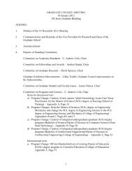
Figure 8a and b: Liquid Mass Flow Rate Versus Heat Input to the Bubble Pump <strong>for</strong> Different<br />
Lift Tube Diameters and System Pressure Conditions.<br />
183<br />
Q BP [W]
m L [kg/s]<br />
0.11<br />
Pressure VS Mass Flow Rate<br />
0.108<br />
0.106<br />
0.104<br />
0.102<br />
0.1<br />
0 0.1 0.2 0.3 0.4 0.5 0.6 0.7<br />
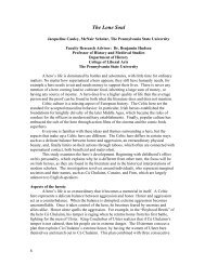
Figure 9: Liquid Mass Flow Rate Versus System Pressure with Lift Tube Diameter of 1 inch<br />
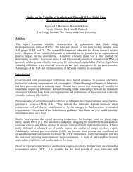
Figures 7 through 9 show the results of parametric studies <strong>for</strong> the <strong>bubble</strong> <strong>pump</strong> <strong>design</strong> <strong>for</strong><br />
integration with a <strong>solar</strong> thermal <strong>hot</strong> <strong>water</strong> heating <strong>system</strong>. As shown in Figure 7, as the diameter<br />
<strong>for</strong> a <strong>bubble</strong> <strong>pump</strong> <strong>design</strong> increases, the mass flow rate of the liquid being <strong>pump</strong>ed through the<br />
<strong>system</strong> increases to a peak value and then decreases again. As this occurs, the two phase flow<br />
regime changes from churn to slug and lastly to bubbly flow. With a lift tube 1 cm in diameter,<br />
the <strong>system</strong> is operating in churn flow at an average <strong>solar</strong> energy input of 700 W/m^2 and the<br />
output flow rate is 1.8 liters per hour. A lift tube of diameter of 3 cm will result in the highest <strong>hot</strong><br />
<strong>water</strong> mass flow rate output of about 7 liter per hour. However, it is unrealistic to have such high<br />
<strong>solar</strong> energy input throughout the day everyday. Figure 8 shows the variation in liquid mass flow<br />
rate or a range of heat transfer rates into the <strong>system</strong>. As the diameter increases more, the two<br />
phase flow regime becomes bubbly flow. Thus, having a lift tube of just less than 3 cm, <strong>for</strong><br />
instance 1 inch in diameter, will likely produce more consistant output from the <strong>bubble</strong> <strong>pump</strong><br />
SHWS throughout the year while receiving the benefit of an output flow rate of 6 to 6.5 liter per<br />
hour. As the temperature in the day fluctuates, the pressure inside the <strong>system</strong> also changes;<br />
however, the pressure in the <strong>system</strong> can be controlled by the valve in the header where the vapor<br />
collects after the <strong>pump</strong>. As shown in Figure 9, as the pressure of the <strong>system</strong> becomes a stronger<br />
vacuum, the saturated temperature <strong>for</strong> <strong>water</strong> decreases, and the <strong>system</strong> will require less <strong>solar</strong><br />
energy input to <strong>pump</strong> <strong>water</strong>. As the pressure increased to 0.45 bars, the mass flow rate increased<br />
slightly with a smaller diameter lift tube, whereas, the larger diameter lift tubes’ mass flow rate<br />
decreased compare to the 0.366 bar case. On the other hand, the mass flow rate decreases as<br />
pressure increases at a lower <strong>solar</strong> energy heat input. With a pressure of 0.25 bars, the output<br />
mass flow rate of the <strong>system</strong> also provides about 6.5 liter per hour of <strong>hot</strong> <strong>water</strong> output at an<br />
average <strong>solar</strong> energy input. Although pressure is an important parameter of the <strong>system</strong>, with the<br />
optimized tube diameter, the pressure of the <strong>system</strong> has less effect on the <strong>system</strong>. As temperature<br />
184<br />
P [bar]
fluctuates throughout the day, the <strong>hot</strong> <strong>water</strong> mass flow rate output also varies. At a constant<br />
pressure of 0.25 bars of the <strong>system</strong>, and lift tube diameter of 1 inch, it is found that the maximum<br />
mass output flow rate occurs at 800W/m 2 , which is consistent with the other results of at least 6<br />
liter per hour of <strong>hot</strong> <strong>water</strong> output.<br />
CONCLUSIONS AND RECOMMENDATIONS FOR FUTURE WORK<br />
The model results showed that having a 1 inch lift tube operating at a pressure of 0.25 bars can<br />
boost up the mass flow rate output to 6 liter per hour, which is about 6 times the required output.<br />
Further study can be done to more effectively simulate the <strong>system</strong> by adding in models of the<br />
<strong>solar</strong> panel, the time varying impacts of the <strong>solar</strong> insulation fluctuation, and additional lift tubes<br />
to study the detailed optimization of the <strong>bubble</strong> <strong>pump</strong> SHWS. Experimental per<strong>for</strong>mance should<br />
be compared with the resulting model be<strong>for</strong>e further analysis and implementation of <strong>system</strong><br />
changes.<br />
185
REFERENCES<br />
de Cachard, F. and Delhaye, J.M. 1996. A slug-churn model <strong>for</strong> small-diameter airlift <strong>pump</strong>s.<br />
Int. J. Multiphase Flow, Vol. 22, No. 4, pp. 627-649.<br />
Chexal, B.; Merilo, M.; Maulbetsch, M.; Horowitz, J.; Harrison, J.; Westacott, J.; Peterson, C.;<br />
Kastner, W.; and Scmidt, H. 1997. Void Fraction Technology <strong>for</strong> Design and Analysis.<br />
Electric Power Research Institute, Palo Alto, CA.<br />
Clark, N.N. and Dabolt, R.J. 1986. A general <strong>design</strong> equation <strong>for</strong> air lift <strong>pump</strong>s operating in slug<br />
flow. AIChE Journal, Vol. 32, No. 1, pp. 56-64.<br />
Haines et al. 1984. Self-<strong>pump</strong>ing Solar Heating System with Geyser Pumping Action. United<br />
States Patent, Patent Number: 4478211.<br />
Hasan, A. R., 1987. Void Fraction in Bubbly, Slug, and Churn Flow in Vertical Two-phase Upflow.<br />
Chem. Eng. Comm. Vol. 66, pp.101-111.<br />
van Housen, 2010. Adaptive Self Pumping Solar Hot Water Heating System with Overheat<br />
Protection. United States Patent, Patent Number: 7798140 B2.<br />
Hewitt, G.F., and Roberts, D.N. 1969. Studies of two-phase flow patterns by simultaneous x-ray<br />
and flash p<strong>hot</strong>ography. AERE-M 2159, HMSO.<br />
Li, X.; Chung H. and Jeong H., 2008. Numerical Simulation of Bubble’s Motion in Vertical<br />
Tube. EngOpt2008, International Conference on Engineering Optimization<br />
Nicklin, D.J. and Davidson, J.F. 1962. The onset of instability in two-phase slug flow.<br />
Presented at a Symp. on Two-phase flow, Inst. Mech. Engrs, London, paper No 4.<br />
Nicklin, D.J.; Wilkes, M.A. and Davidson, M.A. 1962. Two-phase flow in vertical tubes. Trans.<br />
Instn. Chem. Engrs., Vol. 40, pp. 61-68.<br />
REUK, 2010. REUK Solar Website: http://www.reuk.co.uk/Thermosyphon-Solar-Water-<br />
Heating.htm Accessed, June, 2011.<br />
SOL P, 2011. SOL Perpetua Website: http://www.<strong>bubble</strong>action<strong>pump</strong>s.com Accessed, June,<br />
2011.<br />
Sunnovations, 2010. Sunnovations Website: http://www.sunnovations.com/ Accessed, June,<br />
2011.<br />
Taitel, Y. and Bornea D. 1980. Modelling Flow Pattern Transition <strong>for</strong> Steady Upward Gas-<br />
Liquid Flow in Vertical Tubes. The American Instn. Of Chem. Engrs.<br />
Tootoo, 2008. Passive Solar Heating System Website: http://www.tootoo.com/s-ps/passive-<strong>solar</strong><strong>water</strong>-heating-<strong>system</strong>--p-994827.html<br />
Accessed, June, 2011.<br />
US Energy, 2009. US Energy Consumption by Sector Website: http://colli239.fts.educ.msu.edu/<br />
Accessed, June, 2011.<br />
186
White, S.J., 2001. Bubble Pump Design and Per<strong>for</strong>mance. Georgia Institute of Technology<br />
Mech. Engr., Masters Thesis.<br />
WWI, 2011. World Watch Institute Website: http://www.worldwatch.org Accessed, June, 2011.<br />
Zuber, N. and Findlay, J. 1965. Average volumetric concentration in two-phase flow <strong>system</strong>s. J.<br />
of Heat Transfer, Vol. 87, pp. 453-468.<br />
187