Development of Tools to Improve Exposure ... - Trent University
Development of Tools to Improve Exposure ... - Trent University
Development of Tools to Improve Exposure ... - Trent University

Create successful ePaper yourself
Turn your PDF publications into a flip-book with our unique Google optimized e-Paper software.
<strong>Development</strong> <strong>of</strong> <strong>Tools</strong> <strong>to</strong> <strong>Improve</strong> <strong>Exposure</strong> Estimation<br />
for Use in Ecological Risk Assessment<br />
The TaPL3 Upgrade<br />
Report <strong>to</strong> Environment Canada<br />
CEMC Report No. 200303<br />
Prepared by:<br />
Eva Webster, Jennifer Hubbarde, Don Mackay,<br />
Linda Swans<strong>to</strong>n, Adam Hodge<br />
Canadian Environmental Modelling Centre<br />
<strong>Trent</strong> <strong>University</strong><br />
Peterborough, Ontario K9J 7B8<br />
CANADA
<strong>Development</strong> <strong>of</strong> <strong>Tools</strong> <strong>to</strong> <strong>Improve</strong> <strong>Exposure</strong> Estimation<br />
for Use in Ecological Risk Assessment<br />
Report <strong>to</strong> Environment Canada<br />
Contract No. K2251-2-0004<br />
Report 1<br />
The TaPL3 Upgrade<br />
September 30, 2003<br />
Prepared by:<br />
Eva Webster, Jennifer Hubbarde, Don Mackay,<br />
Linda Swans<strong>to</strong>n, Adam Hodge<br />
Canadian Environmental Modelling Centre<br />
<strong>Trent</strong> <strong>University</strong><br />
Peterborough, Ontario<br />
K9J 7B8<br />
EC Departmental Representatives:<br />
Don Gutzman<br />
Head, <strong>Exposure</strong> Section<br />
Chemical Evaluation Division<br />
Existing Substances Branch<br />
Andy Atkinson<br />
Head, New Chemicals Evaluation Section<br />
Chemical Evaluation Division<br />
New Substances Branch<br />
Environment Canada<br />
Place Vincent Massey, 14 th Floor<br />
Hull PQ<br />
K1A 0H3<br />
EC Contracting Authority:<br />
Robert Chenier<br />
Env. Protection Service<br />
Chemical Evaluation Division<br />
351 St. Joseph Blvd 14 th Fl<br />
Hull PQ<br />
K1A 0H3
Table <strong>of</strong> Contents:<br />
Executive Summary<br />
List <strong>of</strong> Tables<br />
List <strong>of</strong> Figures with Captions<br />
Introduction<br />
Study Objectives<br />
Background<br />
TaPL3 Model Upgrades<br />
Temperature Variation<br />
Terrestrial Vegetation<br />
Extent <strong>of</strong> “Grasshopping”<br />
Application <strong>of</strong> TaPL3 version 3.00<br />
Conclusion<br />
Chemical Properties<br />
Environmental Properties<br />
Emissions<br />
Results for the Hypothetical Chemicals<br />
Temperature Variation<br />
Partitioning Variants <strong>of</strong> X<br />
Summary for Chemical X<br />
Results for Selected DSL Chemicals<br />
Future Research Directions<br />
References
List <strong>of</strong> Tables<br />
Table 1:<br />
Additional information needed for the inclusion <strong>of</strong> a vegetation compartment.<br />
Table 2:<br />
Foliage-air transport D value calculations.<br />
Table 3:<br />
Properties <strong>of</strong> selected chemicals.<br />
Table 4:<br />
Environmental properties.<br />
List <strong>of</strong> Figures with Captions<br />
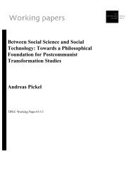
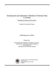
Figure 1:<br />
The partitioning tendency <strong>of</strong> X (x), benzo[a]pyrene (square), chlorobenzene (triangle),<br />
hexachlorobenzene (star), and 2,3,7,8-TCDD (circle). The diagonal lines represent lines <strong>of</strong><br />
constant log K OA . Chemicals in the upper left tend <strong>to</strong> partition in<strong>to</strong> air, in the lower left <strong>to</strong> water,<br />
and in the lower right <strong>to</strong> octanol.<br />
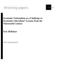
Figure 2:<br />
The three key model outcomes for chemical X and its partitioning variants. The solid square<br />
symbols indicate the presence <strong>of</strong> vegetation in the modelled environment; the open triangle<br />
symbols indicate the absence <strong>of</strong> vegetation.<br />
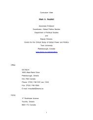
Figure 3:<br />
The persistence, P, characteristic travel distance in air, L A , and average number <strong>of</strong> hops<br />
experienced by a single molecule, H, for each <strong>of</strong> four substances; benzo[a]pyrene,<br />
chlorobenzene, hexachlorobenzene, and 2,3,7,8-TCDD. The open triangle symbols indicate the<br />
case <strong>of</strong> no vegetation present while the solid square symbols indicate the presence <strong>of</strong> vegetation.<br />
The horizontal axis represents decreasing temperature (a northward movement) from 25 <strong>to</strong> 5 C.
EXECUTIVE SUMMARY<br />
As a result <strong>of</strong> a series <strong>of</strong> research projects at the CEMC which included collaborations with the<br />
<strong>University</strong> <strong>of</strong> Osnabrück, TaPL3, an evaluative model describing the transport and persistence <strong>of</strong><br />
organic chemicals, was developed. It has been available from the CEMC website since 2000. As a<br />
result <strong>of</strong> use by a number <strong>of</strong> individuals and agencies, the need for certain upgrades or improvements<br />
is apparent.<br />
In this project, the TaPL3 model was upgraded <strong>to</strong> include provision for temperatures <strong>to</strong> be varied,<br />
improved treatment <strong>of</strong> vegetation, and an alternate descrip<strong>to</strong>r for the potential for long-range<br />
transport. Enthalpies <strong>of</strong> phase change are used <strong>to</strong> adjust chemical partitioning data <strong>to</strong> the<br />
temperature <strong>of</strong> the modelled environment. Reaction activation energies are used <strong>to</strong> adjust chemical<br />
degradation rate constants. Vegetation was added as a single primary medium with active transport<br />
mechanisms between air and foliage. The average number <strong>of</strong> air-<strong>to</strong>-surface cycles, referred <strong>to</strong><br />
colloqually as “hops”, experienced by a single molecule is calculated as an estimate <strong>of</strong> the potential<br />
for long-rang transport. This new version <strong>of</strong> the model will be made freely and publically available<br />
from the CEMC website (http://www.trentu.ca/cemc/).<br />
Hypothetical chemicals were used <strong>to</strong> explore the key model outcomes <strong>of</strong> persistence, P, characteristic<br />
travel distance in air, L A , and extent <strong>of</strong> hopping, H. This was followed by a similar investigation with<br />
four dissimilar chemicals from the DSL (Domestic Substances List). Several future research<br />
directions are suggested including improved treatment <strong>of</strong> bioturbation in soil.
1 INTRODUCTION<br />
This report is the first in a series <strong>of</strong> three reports prepared in fulfilment <strong>of</strong> Contract K2251-2-0004<br />
“<strong>Development</strong> <strong>of</strong> <strong>Tools</strong> <strong>to</strong> <strong>Improve</strong> <strong>Exposure</strong> Estimation for Use in Ecological Risk Assessment”.<br />
Here, changes <strong>to</strong> the TaPL3 (Transport and Persistence Level III) model are described. Hypothetical<br />
chemicals and selected substances from the DSL are used <strong>to</strong> demonstrate the utility <strong>of</strong> the upgraded<br />
model. In applying the model three key outcomes are examined; the persistence, P, the characteristic<br />
travel distance in air, L A , and the average number <strong>of</strong> hops experienced by a single molecule, H.<br />
1.1 Study Objectives<br />
The objectives <strong>of</strong> this work were stated in the contract as follows.<br />
“To improve the Transport and Persistence Level III (TaPL3) Model for the use <strong>of</strong><br />
Environment Canada. The TaPL3 model is an evaluative <strong>to</strong>ol <strong>to</strong> be used in the detailed<br />
assessment <strong>of</strong> chemicals for persistence and potential for long-range transport in a mobile<br />
medium, either air, or water in a Level III (steady-state) environment. A number <strong>of</strong><br />
improvements are <strong>to</strong> be made <strong>to</strong> the model including provision for temperatures <strong>to</strong> be varied,<br />
terrestrial characteristics <strong>to</strong> be better defined (including, differentiating between prairie,<br />
deciduous and coniferous forests) and an estimate made <strong>of</strong> the distribution <strong>of</strong> transport<br />
distances and the extent <strong>of</strong> "grasshopping". Selected substances from the DSL will be used <strong>to</strong><br />
demonstrate the utility <strong>of</strong> the upgraded model.”<br />
1.2 Background<br />
The persistence, P, <strong>of</strong> a substance is now widely defined as its longevity in the environment with<br />
removal only by degradation. This is not a directly measurable property <strong>of</strong> the substance but can be<br />
calculated using a steady-state environmental model as suggested by Webster et al (1998). It has also<br />
been suggested that the potential for long-range transport (LRT) can be calculated by such a model<br />
-1-
as a characteristic travel distance in air, L A (Beyer et al, 2000). While it is not possible <strong>to</strong> compare<br />
the values calculated for a single substance with any measured value, substances can be ranked based<br />
on either P or L A and this ranking can be compared <strong>to</strong> either evidence <strong>of</strong> longevity or <strong>to</strong> evidence <strong>of</strong><br />
transport <strong>to</strong> remote regions.<br />
The original TaPL3 model was created <strong>to</strong> facilitate the calculation <strong>of</strong> P and L A for organic substances<br />
and is based on the following publications: the fugacity concept initially proposed in 1979 (Mackay,<br />
1979) and detailed in Mackay (2001); the calculation <strong>of</strong> persistence using a Level III model (Webster<br />
et al 1998); and the calculation <strong>of</strong> L A using a Level III model ( Beyer et al, 2000).<br />
2 TAPL3 MODEL UPGRADES<br />
Since the development <strong>of</strong> the TaPL3 model (version 2.10, released June 2000), our understanding<br />
<strong>of</strong> the influence <strong>of</strong> temperature and <strong>of</strong> vegetation has increased. With this increased understanding<br />
the model results are refined by reducing the simplicity <strong>of</strong> the assumptions in the model. In addition,<br />
a new way <strong>of</strong> describing chemical transport as a “hopping” between mobile and stationary media has<br />
been developed and refined. It is hoped that the inclusion <strong>of</strong> this new descrip<strong>to</strong>r will improve<br />
understanding <strong>of</strong> the long-range transport processes.<br />
2.1 Temperature Variation<br />
The temperature <strong>of</strong> the environment is known <strong>to</strong> influence both the physical-chemical properties <strong>of</strong><br />
substances and their ability <strong>to</strong> degrade. Properties are typically measured at indoor temperatures<br />
<strong>of</strong>ten a standard <strong>of</strong> 25/C. This focus on property measurement at indoor temperatures is a direct<br />
result <strong>of</strong> the cost <strong>of</strong> making such measurements and the large numbers <strong>of</strong> substances <strong>to</strong> be analyzed.<br />
In recent years has there been an effort <strong>to</strong> extend this in<strong>to</strong> more typical outdoor temperatures. The<br />
temperature dependence <strong>of</strong> the partitioning properties <strong>of</strong> sets <strong>of</strong> substances such as the<br />
chlorobenzenes, PCBs, and PAHs have been reported by Bahadur et al (1997, 1999), Shiu et al<br />
(1997), and Shiu and Ma (2000). Beyer et al (2002) produced a more comprehensive study <strong>of</strong> 50,<br />
-2-
mostly aromatic, substances. The majority <strong>of</strong> effort in this field has focussed on the temperature<br />
dependence <strong>of</strong> partitioning properties and thus there is confidence in the correlation and the ability<br />
<strong>of</strong> users <strong>to</strong> obtain data. This is not the case for the temperature dependence <strong>of</strong> degradation rates.<br />
Chemical degradation in the environment is influenced by many fac<strong>to</strong>rs including the microbial<br />
community present, light intensity and duration, and temperature. These cause the degradation rate<br />
<strong>of</strong> a substance <strong>to</strong> vary by as much as an order <strong>of</strong> magnitude from place <strong>to</strong> place and from season <strong>to</strong><br />
season. The temperature dependence <strong>of</strong> hydroxyl reaction rates have been measured by Anderson<br />
and Hites (1996), and Brubaker and Hites (1997, 1998a, 1998b) for a small set <strong>of</strong> substances.<br />
As outlined by Beyer et al (2000) and further detailed in Beyer et al (2003) and Gouin (2003),<br />
temperature has a complex effect on persistence, P, and characteristic travel distance, L A . At lower<br />
temperatures, chemical typically partitions more strongly <strong>to</strong> water and soil decreasing L A by transport<br />
from the mobile <strong>to</strong> the stationary media. The persistence tends <strong>to</strong> increase since, for most chemicals,<br />
their half-life in air is shorter than in other media. In addition, degradation processes in all media<br />
tend <strong>to</strong> take place more slowly thus further increasing P. An increase in longevity has the opposite<br />
effect on L A . The relative strength <strong>of</strong> these opposing effects will determine whether L A increases or<br />
decreases with decreasing temperature. Thus if we were <strong>to</strong> consider only the temperature effects on<br />
partitioning, the increase in P would be under-estimated and neither P nor L A would be correct for<br />
the temperature <strong>of</strong> the environment. If all chemicals were equally affected, neither correction would<br />
be required since only the relative ranking has meaning. However, the enthalpies <strong>of</strong> phase change<br />
and reaction activation energies are chemical specific. The relative rankings <strong>of</strong> substances for P and<br />
L A are expected <strong>to</strong> be affected by temperature; the direction and magnitude <strong>of</strong> changes in P and L A<br />
will not be the same for all chemicals.<br />
The TaPL3 model was modified include the following equation which is based on the conventioanl<br />
Arrhenius, or Van’t H<strong>of</strong>f, equation.<br />
P e = P o e<br />
(Ea (1 / To - 1 / Te) / R)<br />
where P e is the property at the environment temperature, T e (K), P o is the property at the chemical<br />
data collection temperature, T o , E a (J/mol) is the enthalpy <strong>of</strong> phase change or reaction activation<br />
-3-
energy, and R is the gas constant (8.314 J/mol.K). This correction is applied separately <strong>to</strong> each <strong>of</strong><br />
the octanol-water partition coefficient, K OW , and the air-water partition coefficient K AW , and <strong>to</strong> the<br />
degradation rate constants. This represents an implementation <strong>of</strong> the research <strong>of</strong> Mackay (2001) and<br />
Beyer et al (2000, 2003).<br />
While the chemical properties are now corrected for the environment temperature, it should be noted<br />
that sub-zero temperatures are not treated. Ice formation and snow cover are expected <strong>to</strong> control both<br />
chemical partitioning and degradation rates in Canadian winters. The ChemCAN model (version<br />
6.00) provides a simplistic treatment <strong>of</strong> winter conditions by preventing selected transport<br />
mechanisms (Webster et al, 2003). The effects <strong>of</strong> snow cover are currently being studied by The<br />
Wania Group (http://www.scar.u<strong>to</strong><strong>to</strong>n<strong>to</strong>.ca/~wania/ ). Sub-zero temperature effects are quite<br />
complex and not yet well-unders<strong>to</strong>od. To avoid mis-leading results they were not included in the<br />
TaPL3 model. As the science advances, this can be added <strong>to</strong> a future version <strong>of</strong> the model.<br />
2.2 Terrestrial Vegetation<br />
Typically environmental models <strong>of</strong> chemical fate include three or four primary media: air, water,<br />
soil, and sometimes sediment. While this has been sufficient for most purposes <strong>to</strong> date, it has been<br />
acknowledged that most <strong>of</strong> the landmass <strong>of</strong> the planet is covered by vegetation. This fact has never<br />
been so evident as with the many satellite images now being produced. Introducing vegetation<br />
introduces a degree <strong>of</strong> complexity, but it is not entirely clear what level <strong>of</strong> detail and complexity is<br />
most appropriate when examining issues <strong>of</strong> chemical persistence and tendency <strong>to</strong> travel large<br />
distances.<br />
In adding vegetation <strong>to</strong> a steady-state environmental model two extremes have been explored. The<br />
ChemCAN model (Mackay et al, 1991; Webster et al, 2003) includes the simplest assumption <strong>of</strong><br />
vegetation; foliage in equilibrium with the air. This assumption produces values for P and L A<br />
identical <strong>to</strong> a four-compartment model. Recent work by Gouin (2003) has indicated that the a fourcompartment<br />
model fails <strong>to</strong> explain the extent <strong>of</strong> long-range transport observed. Other authors have<br />
-4-
suggested the inclusion <strong>of</strong> as many as four vegetation compartments coupled <strong>to</strong> soils specific <strong>to</strong> the<br />
vegetation type and interactions with the soils in addition <strong>to</strong> the interactions with air (Cousins and<br />
Mackay, 2001; Cahill and Mackay, 2003). With each addition in complexity the model requires<br />
additional information. To avoid increasing the data demands beyond what can be obtained with a<br />
reasonable degree <strong>of</strong> effort, the increase in complexity was limited <strong>to</strong> the addition <strong>of</strong> a single<br />
vegetation compartment as a primary medium. This increased the number <strong>of</strong> simultaneous equations<br />
from four <strong>to</strong> five with a separate fugacity being sought for each primary medium. The vegetation is<br />
assumed <strong>to</strong> have interactions only with the air through foliage by three processes: aerosol deposition,<br />
rain, and diffusion. Chemical is also assumed <strong>to</strong> be degraded on the leaf surface. No root tissues are<br />
included and there is no run<strong>of</strong>f from the leaves <strong>to</strong> the soil. The foliage is considered <strong>to</strong> “float” above<br />
the soil leaving the entire soil surface available for interactions with the air, and <strong>to</strong> receive rain<br />
unimpeded by the presence <strong>of</strong> the vegetation.<br />
Table 1 shows the additional information required by the model and Table 2 details the calculations<br />
performed. The value <strong>of</strong> the input parameters such as leaf biomass, lipid fraction, and leaf area index<br />
can be used <strong>to</strong> differentiate between ecosystems such as prairie, deciduous and coniferous forests.<br />
2.3 Extent <strong>of</strong> “Grasshopping”<br />
In the past, a characteristic travel distance in air, L A , has been used <strong>to</strong> describe the long-range<br />
transport potential <strong>of</strong> a substance (Beyer et al 2000). While useful for ranking substances, this is not<br />
an entirely satisfying description. Wania and Mackay (1996, 1997) have described the travel path<br />
<strong>of</strong> a molecule with seasonal temperature changes as a series <strong>of</strong> “hops”. The molecule is viewed as<br />
undergoing a series <strong>of</strong> deposition and evaporation process pairs, each process pair constituting a<br />
single hop. This gives a more realistic and intuitively satisfying description <strong>of</strong> the events responsible<br />
for long range transport and was further developed in Gouin (2003). Here this “grasshopping”<br />
description is extended from essentially a two-compartment environmental system <strong>to</strong> the five<br />
primary media <strong>of</strong> the new TaPL3 model.<br />
-5-
The average number <strong>of</strong> hops experienced by a single molecule from the time <strong>of</strong> release in<strong>to</strong> the<br />
environment <strong>to</strong> degradation, H, is given by<br />
H = (N W,A + N S,A + N V,A ) / E<br />
where N W,A is the water <strong>to</strong> air transfer rate, N S,A is the soil <strong>to</strong> air transfer rate, N V,A is the vegetation<br />
<strong>to</strong> air transfer rate, and E is the rate <strong>of</strong> emission (<strong>to</strong> air). Since consistent units are used for all rates,<br />
H is a unitless ratio. Note that this equation applies only when the emission is entirely <strong>to</strong> air.<br />
A related parameter, “stickiness”, S, is calculated as the fraction <strong>of</strong> deposited chemical which never<br />
returns <strong>to</strong> the air.<br />
S W = ( N AW - N WA ) / N AW<br />
where S W is the stickiness <strong>of</strong> water. This is a measure <strong>of</strong> the chemical’s tendency <strong>to</strong> remain in the<br />
water and not return <strong>to</strong> the air compartment. The stickiness <strong>of</strong> soil, S S , and <strong>of</strong> vegetation, S V , are<br />
similarly calculated.<br />
3 APPLICATION OF TAPL3 (VERSION 3.00)<br />
The persistence, P, characteristic travel distance in air, L A , and the average number <strong>of</strong> hops<br />
experienced by a single molecule, H, are examined for two groups <strong>of</strong> chemicals, one consists <strong>of</strong><br />
hypothetical chemicals, and the other is four chemicals selected from the DSL.<br />
3.1 Chemical Properties<br />
The hypothetical chemical, X, first defined by Webster et al (1998) is used here <strong>to</strong> explore <strong>of</strong> the<br />
impact <strong>of</strong> the changes made <strong>to</strong> the TaPL3 model. This chemical has properties similar <strong>to</strong><br />
tetrachlorobenzene but has degradation half-lives which are set at half the Canadian single-medium<br />
persistence criteria. The degradation half-life in vegetation was assumed <strong>to</strong> be half that in air <strong>to</strong><br />
reflect the tendency <strong>of</strong> the leaf surface <strong>to</strong> be oriented such that pho<strong>to</strong>lysis will be maximized. By<br />
varying log K OW values from 3 <strong>to</strong> 7 and vapour pressures from 0.0072 <strong>to</strong> 72000 Pa two sets <strong>of</strong><br />
hypothetical chemicals are produced. With this wide range <strong>of</strong> partitioning properties simulating<br />
-6-
chemical property space, the key characteristics <strong>of</strong> P, L A , and H, and the effects <strong>of</strong> including<br />
vegetation as a primary medium were examined.<br />
Four substances were selected from the DSL <strong>to</strong> continue the examination <strong>of</strong> P, L A , and H in<strong>to</strong> the<br />
realm <strong>of</strong> real chemicals.<br />
The properties <strong>of</strong> X and the substances from the DSL used here are given in Table 3. The partitioning<br />
tendency <strong>of</strong> the five chemicals in shown in Figure 1. Chemical-specific enthalpies <strong>of</strong> phase change<br />
were used <strong>to</strong> adjust K OW and K AW for temperature, however, activation energies were not available.<br />
The values are typical <strong>of</strong> organic substances and are sufficient <strong>to</strong> show temperature effects. However,<br />
for an assessment, values specific <strong>to</strong> the chemical should be sought.<br />
3.2 Environment Properties<br />
For any set <strong>of</strong> chemical evaluations, a constant environment should be used, but the user should have<br />
the ability <strong>to</strong> define that environment. The TaPL3 (version 3.00) model allows an environment <strong>to</strong><br />
be defined by the user and saved in a database for future use (as in the previously released version<br />
<strong>of</strong> the model). For this study the “EQC - standard environment” (Mackay et al 1996) was used but<br />
with vegetation included for half the simulations as noted. The parameters selected <strong>to</strong> represent<br />
vegetation are considered <strong>to</strong> be reasonable estimates for typical conditions. For specific regions, field<br />
data should be compiled. Table 4 shows the environmental properties.<br />
As a part <strong>of</strong> this study, temperatures ranging from 5 <strong>to</strong> 25 C were examined. Canadian temperatures<br />
are <strong>of</strong>ten lower than this, however, as discussed earlier, <strong>to</strong> avoid the complications <strong>of</strong> ice formation<br />
and snow cover, only temperatures above freezing were used.<br />
-7-
3.3 Emissions<br />
Two emission scenarios are considered in the TaPL3 model; <strong>to</strong> air and (separately) <strong>to</strong> water. In the<br />
case <strong>of</strong> emission <strong>to</strong> air, air is considered <strong>to</strong> be the sole mobile medium and the characteristic travel<br />
distance in air, L A , is calculated. Similarly, in the case <strong>of</strong> emission <strong>to</strong> water, water is considered <strong>to</strong><br />
be the sole mobile medium and the characteristic travel distance in water, L W is calculated. Since<br />
chemicals are emitted <strong>to</strong> other media, it would be interesting <strong>to</strong> consider other scenarios. This will<br />
be the <strong>to</strong>pic <strong>of</strong> subsequent study. Here, only the more commonly considered and better unders<strong>to</strong>od<br />
case <strong>of</strong> air as the mobile medium is examined.<br />
3.4 Results for the Hypothetical Chemicals<br />
The three key model outcomes (P, L A , H) for hypothetical chemical X and its partitioning variants<br />
are shown in Figure 2 both with and without vegetation. In the absence <strong>of</strong> vegetation, model results<br />
are consistent with the previously released version 2.10 <strong>of</strong> the model.<br />
3.4.1 Temperature Variation<br />
Chemical X was assigned enthalpies <strong>of</strong> phase change and reaction activation energies as shown in<br />
Table 3. Over the range <strong>of</strong> temperatures from 25 <strong>to</strong> 5/C as temperature decreases K OW increases, i.e.,<br />
the chemical partitions more strongly <strong>to</strong> octanol (soil, sediment and vegetation), K AW increases, i.e.,<br />
the chemical partitions less strongly <strong>to</strong> air, and reaction rate constants decrease, i.e., the half-lives<br />
increase, or degradation happens more slowly. Figure 2 shows the relative change in key model<br />
outcomes with decreasing temperature for chemical X. The horizontal axis shows decreasing<br />
temperature <strong>to</strong> reflect a molecule’s journey from south <strong>to</strong> north (in the Northern Hemisphere). As<br />
temperature decreases, P, L A , and H all increase. This can be seen as the combined effect <strong>of</strong> the<br />
general increase in media half-lives and the partitioning out <strong>of</strong> the air in<strong>to</strong> media where degradation<br />
happens more slowly. The stickiness <strong>of</strong> vegetation increases with decreasing temperature. As the<br />
stickiness <strong>of</strong> the vegetation increases, the average number <strong>of</strong> hops experienced by a molecule<br />
-8-
decreases. In the presence <strong>of</strong> vegetation, P and H are greater for chemical X and L A is less. The<br />
temperature effect is enhanced by the presence <strong>of</strong> vegetation which adds <strong>to</strong> the <strong>to</strong>tal volume <strong>of</strong><br />
octanol-like media in the modelled environment.<br />
In summary, a molecule <strong>of</strong> chemical X has an increased longevity, travels increasing distances, and<br />
experiences more hops as it moves from warmer <strong>to</strong> cooler regions in its journey northwards.<br />
3.4.2 Partitioning Variants <strong>of</strong> X<br />
The environment temperature was set at 20/C and two sets <strong>of</strong> chemicals were used <strong>to</strong> examine the<br />
effects <strong>of</strong> partitioning properties on P, L A , and H with and without vegetation included in the<br />
modelled environment.<br />
Using the set <strong>of</strong> chemicals defined by varying log K OW from 3 <strong>to</strong> 7 and retaining all other properties<br />
<strong>of</strong> chemical X, in the absence <strong>of</strong> vegetation, P increases with K OW while L A and H remain relatively<br />
constant (Figure 2). By contrast, when vegetation is included in the modelled environment, P and<br />
H are seen <strong>to</strong> peak at log K OW values <strong>of</strong> 6 and 5 respectively and L A declines after log K OW 5. At<br />
higher K OW values the chemical partitions more strongly in<strong>to</strong> vegetation where the half-life is<br />
shortest, thus reducing P. This partitioning <strong>to</strong> vegetation is seen in the increased stickiness. With<br />
increased partitioning in<strong>to</strong> vegetation, i.e., out <strong>of</strong> the mobile medium (air), L A is reduced. Both the<br />
shift in partitioning tendency out <strong>of</strong> the mobile medium and the increased degradation reduce H.<br />
Similarly, using the set <strong>of</strong> chemicals defined by varying the vapour pressure from 0.0072 <strong>to</strong> 72000<br />
Pa and retaining all other properties <strong>of</strong> chemical X in the presence <strong>of</strong> vegetation, persistence<br />
declines, L A increases, and H peaks at about 0.72 Pa as shown in Figure 2. The presence <strong>of</strong><br />
vegetation enhances the effect on P, but without vegetation no effect is seen for L A and H.<br />
Varying vapour pressure across the above range is equivalent for chemical X <strong>to</strong> varying log K AW<br />
from -3.3 <strong>to</strong> 3.7. As K AW increases, these substances partition more in<strong>to</strong> air and less in<strong>to</strong> water<br />
-9-
making them more available for transport <strong>to</strong> vegetation which is modelled as interacting only with<br />
air. At very low values <strong>of</strong> K AW , a high stickiness is seen due <strong>to</strong> the reduced tendency <strong>to</strong> partition <strong>to</strong><br />
air. At very high values <strong>of</strong> K AW , a high stickiness is seen due <strong>to</strong> an increased availability <strong>of</strong> the<br />
substance. Thus the valley-shaped curve seen in Figure 2 results.<br />
3.4.3 Summary for Chemical X<br />
Figure 2 shows the effect <strong>of</strong> environmental temperature on a single chemical with and without<br />
vegetation included in the modelled environment, and how vegetation interacts on the partitioning<br />
and degradation properties <strong>of</strong> the chemical. A more complete representation <strong>of</strong> chemical space,<br />
including a range <strong>of</strong> degradation half-lives, would further elucidate the effects <strong>of</strong> vegetation as it is<br />
represented in TaPL3 version 3.00 on the key model outcomes <strong>of</strong> P, L A , and H and by the stickiness<br />
<strong>of</strong> vegetation.<br />
3.5 Results for Selected DSL Chemicals<br />
Figure 3 shows P, L A , and H, for each <strong>of</strong> four substances; benzo[a]pyrene (B[a]p), chlorobenzene<br />
(CB), hexachlorobenzene (HCB), and 2,3,7,8-tetrachloro-dibenzo-p-dioxin (TCDD). The open<br />
triangle symbols indicate the case <strong>of</strong> no vegetation present while the solid square symbols indicate<br />
the presence <strong>of</strong> vegetation. The horizontal axis represents decreasing temperature (a northward<br />
movement) from 25 <strong>to</strong> 5 /C for each chemical in the EQC standard environment.<br />
The two scenarios, with and without vegetation, show a general consistency, but with different scales<br />
for these three chemicals. The change in the stickiness <strong>of</strong> vegetation is small over the range <strong>of</strong><br />
temperatures studied.<br />
B[a]p: 0.99 <strong>to</strong> 1<br />
CB: 0.009 <strong>to</strong> 0.002<br />
HCB: 0.0002 <strong>to</strong> 0.0014<br />
TCDD: 0.94 <strong>to</strong> 1<br />
-10-
The difference in the values for P, L A , and H between the vegetation scenario and the no vegetation<br />
scenario are in agreement with studies showing the important role <strong>of</strong> vegetation for some chemicals.<br />
Further study would be needed <strong>to</strong> ascertain the impact <strong>of</strong> the inclusion <strong>of</strong> vegetation in the modelled<br />
environment on any chemical ranking for P, L A , and H. With this small set <strong>of</strong> very different<br />
chemicals, no change in rank can be expected as the differences between the chemicals are greater<br />
than the influence <strong>of</strong> vegetation.<br />
4 CONCLUSION<br />
The TaPL3 model was successfully upgraded <strong>to</strong> include provision for the temperature <strong>of</strong> the<br />
modelled environment <strong>to</strong> be varied, vegetation as a primary medium with active chemical exchange<br />
with air, and an estimate <strong>of</strong> the extent <strong>of</strong> “grasshopping”. This new version <strong>of</strong> the model will be<br />
made freely and publically available from the CEMC website (http://www.trentu.ca/cemc/).<br />
The limited application <strong>of</strong> this model <strong>to</strong> a set <strong>of</strong> hypothetical chemicals and four DSL chemicals<br />
demonstrates some <strong>of</strong> the potential impact <strong>of</strong> the changes <strong>to</strong> the model on the key outcomes <strong>of</strong><br />
persistence, P, and characteristic travel distance in air, L A , and the average number <strong>of</strong> hops<br />
experienced by a single molecule, H. For some substances, the inclusion <strong>of</strong> vegetation as a primary<br />
medium in the model will affect the values <strong>of</strong> P, L A , and H. Temperature had a smaller effect than<br />
the inclusion <strong>of</strong> vegetation. Chemical cycling between stationary and mobile media, as described by<br />
H and the stickiness <strong>of</strong> vegetation, provides further insight in<strong>to</strong> chemical fate in the environment.<br />
-11-
5 FUTURE RESEARCH DIRECTIONS<br />
Several desirable research directions for the future are apparent.<br />
1. The compiling <strong>of</strong> field data <strong>to</strong> confirm trends identified by the model and thus contribute <strong>to</strong><br />
validation and credibility.<br />
2. Using emission scenarios other than <strong>to</strong> air only when determining long-range transport.<br />
3. Performing a more detailed investigation <strong>of</strong> the effects <strong>of</strong> each vegetation parameter.<br />
4. Investigating the complex processes caused by the presence <strong>of</strong> snow and including these<br />
processes in models <strong>to</strong> simulate sub-zero climates.<br />
5. It has been demonstrated that the present treatment <strong>of</strong> soil as a single well-mixed layer is<br />
excessively simplistic. The calculation <strong>of</strong> the resistence <strong>to</strong> uptake and volatilization requires<br />
that the chemical diffuse a distance <strong>of</strong> half the soil depth. Bioturbation by soil-dwelling<br />
organisms can assist this transport process and can enhance the rates <strong>of</strong> uptake and release.<br />
6. TaPL3 is a true steady-state model which describes conditions when this steady-state is<br />
reached. For substances <strong>of</strong> high K OA this time may be very long i.e., decades, thus in the<br />
immediate future the actual values <strong>of</strong> P, L, and H may be different. Investigating this effect<br />
would require a dynamic, or Level IV, model which is considerably more complex and data<br />
intensive, but could provide additional, valuable insights in<strong>to</strong> chemical’s persistence and<br />
long-range transport.<br />
-12-
REFERENCES<br />
Anderson, P.N., Hites, R.A. 1996. OH Radical Reactions: The Major Removal Pathway for<br />
Polychlorinated Biphenyls for the Atmosphere. Environ. Sci. Technol. 30: 1756-1763.<br />
Bahadur, N.P., Shiu, W.Y., Boocock, D.G.B., Mackay D. 1997. Temperature Dependence <strong>of</strong><br />
Octanol-Water Partition Coefficient for Selected Chlorobenzenes. J. Chem. Eng. Data 42: 685-688.<br />
Bahadur, N., Shiu, W.-Y., Boocock, D., Mackay, D. 1999. Tricaprylin-Water Partition Coefficients<br />
and Their Temperature Dependence for Selected Chlorobenzenes. J. Chem. Eng. Data. 44: 40-43.<br />
Beyer, A., Mackay, D., Matthies, M., Wania, F., Webster, E. 2000. Assessing Long-range Transport<br />
Potential <strong>of</strong> Persistent Organic Pollutants. Environ. Sci. Tech. 34: 699-703.<br />
Beyer, A., Wania, F., Gouin, T., Mackay, D., Matthies, M. 2002. Selecting Internally Consistent<br />
Physical-Chemical Properties <strong>of</strong> Organic Compounds. Environ. Toxicol. Chem. 21: 941-953.<br />
Beyer, A., Wania, F., Gouin, T., Mackay, D., Matthies, M. 2003. Temperature Dependence <strong>of</strong> the<br />
Characteristic Travel Distance. Environ. Sci. Technol. 37: 766-771.<br />
Brubaker, W.W., Hites, R.A. 1998. OH Reaction Kinetics <strong>of</strong> Gas-Phase "- and (-<br />
Hexachlorocyclohexane and Hexachlorobenzene. Environ. Sci. Technol. 32: 766-769.<br />
Brubaker, W.W., Hites, R.A. 1997. Polychlorinated Dibenzo-p-dioxins and Dibenz<strong>of</strong>urans: Gas-<br />
Phase Hydroxyl Radical Reactions and Related Atmospheric Removal. Environ. Sci. Technol. 31:<br />
1805-1810.<br />
Brubaker, W.W., Hites, R.A. 1998. OH Reaction Kinetics <strong>of</strong> Polycyclic Aromatic Hydrocarbons and<br />
Polychlorinated Dibenzo-p-dioxins and Dibenz<strong>of</strong>urans. J. Phys. Chem. 102: 915-921.<br />
Cahill, T.M., Mackay, D. 2003. Complexity in Multimedia Mass Balance Models: When are simple<br />
models adequate and when are more complex models necessary? Environ. Toxicol. Chem. 22: 1404-<br />
1412.<br />
Cousins, I., Mackay, D. 2000. Transport Parameters and Mass Balance Equations for Vegetation in<br />
a Level III Fugacity Model. CEMC Report No. 200001. <strong>Trent</strong> <strong>University</strong>, Peterborough, Ontario.<br />
Cousins, I. T., Mackay, D. 2001. Strategies for including vegetation compartments in multimedia<br />
models. Chemosphere. 44: 643-654.<br />
Gouin, T. 2003. Long-range Transport <strong>of</strong> Organic Contaminants: The role <strong>of</strong> air-surface exchange.<br />
Masters thesis, Applications <strong>of</strong> Modelling in the Natural and Social Sciences Graduate Program,<br />
<strong>Trent</strong> <strong>University</strong>, Peterborough, Ontario.<br />
-13-
Mackay, D. 1979. Finding Fugacity Feasible. Environ. Sci. Technol. 13: 1218.<br />
Mackay, D., Paterson, S., Tam, D.D., 1991. Assessments <strong>of</strong> Chemical Fate in Canada:<br />
Continued <strong>Development</strong> <strong>of</strong> a Fugacity Model. A report prepared for Health and Welfare Canada.<br />
Mackay D, Paterson, S., Di Guardo, A., Cowan, C.E. 1996. Evaluating the Environmental Fate <strong>of</strong><br />
a Variety <strong>of</strong> Types <strong>of</strong> Chemicals Using the EQC Model Environ. Toxicol. Chem. 15: 1627-1637.<br />
Mackay, D. 2001. “Multimedia Environmental Models: The Fugacity Approach - Second<br />
Edition”, Lewis Publishers, Boca Ra<strong>to</strong>n, pp.1-261.<br />
Shiu, W.Y., Wania F, Hung, H, Mackay, D. 1997. Temperature Dependence <strong>of</strong> Aqueous<br />
Solubility <strong>of</strong> Selected Chlorobenzenes, Polychlorinated Biphenyls and Dibenz<strong>of</strong>uran. J. Chem.<br />
Eng. Data. 42: 293-297.<br />
Shiu, W.Y., Ma, K. 2000. Temperature dependence <strong>of</strong> physical-chemical properties <strong>of</strong> selected<br />
chemicals <strong>of</strong> environmental interest. 1. Mononuclear and polynuclear aromatic hydrocarbons. J.<br />
Phys. Chem. Ref. Data. 29: 41-130.<br />
Wania, F., Mackay, D. 1996. Tracking the Distribution <strong>of</strong> Persistent Organic Pollutants.<br />
Environ. Sci. Technol. 30: 390A-396A.<br />
Wania, F., Mackay, D. 1997. Global Distillation. Our Planet: The United Nations Environment<br />
Programme Magazine for Environmentally Sustainable <strong>Development</strong>. 8: 15-16.<br />
Webster E., Mackay, D., Wania, F. 1998. Evaluating Environmental Persistence. Environ.<br />
Toxicol. Chem. 17: 2148-2158.<br />
Webster, E., Mackay, D., Di Guardo, A., Kane, D., Woodfine, D. 2003. Regional Differences in<br />
Chemical Fate Model Outcome. Chemosphere. (Accepted for publication August, 2003.)<br />
-14-
Table 1: Additional information needed for the inclusion <strong>of</strong> a vegetation compartment.<br />
Chemical properties for vegetation<br />
degradation half-life in vegetation (h)<br />
reaction activation energy(kJ/mol)<br />
Environment properties for vegetation<br />
fraction <strong>of</strong> landmass covered by vegetation<br />
leaf biomass (kg/m 2 )<br />
density <strong>of</strong> leaf tissue (kg <strong>of</strong> vegetation / m 3 <strong>of</strong> vegetation)<br />
lipid fraction (g/g)<br />
leaf area index (m 2 /m 2 )<br />
leaf-air boundary layer mass transfer coefficient (m/h)<br />
fraction <strong>of</strong> rain intercepted by the foliage
Table 2: Foliage-air transport D value calculations (based on Cousins and Mackay 2001).<br />
Diffusion<br />
Rain<br />
Log P C = ((0.704 log K OW - 11.2) + (-3.47 - 2.79 log MM + 0.970 log K OW ))/2<br />
P C is the cuticle permeance (m/s)<br />
MM is the molar mass (g/mol)<br />
U C = 3600 P C / K AW<br />
U C is the mass transfer coefficient through the cuticle (m/h)<br />
D C = A V L Z V U C<br />
D C is for diffusion in<strong>to</strong> the cutin<br />
L is the leaf area index (m 2 /m 2 )<br />
Z V is the fugacity capacity <strong>of</strong> vegetation (mol/m 3 Pa)<br />
D B = A V L Z A U B<br />
D B is for boundary layer diffusion<br />
Z W is the fugacity capacity <strong>of</strong> air (mol/m 3 Pa)<br />
U B leaf-air boundary layer mass transfer coefficient (m/h)<br />
D A = 1/(1/D C +1/D B )<br />
D A is <strong>to</strong>tal diffusion<br />
D R = A V v R Z W U R<br />
Aerosol dry deposition<br />
v R is the volume fraction <strong>of</strong> rain intercepted by the foliage (m 3 /m 3 ), a user input<br />
Z W is the fugacity capacity <strong>of</strong> water (mol/m 3 Pa)<br />
U R is the rain rate (m/h), a user input<br />
D Q = A V v Q Z Q U Q<br />
Aerosol wet deposition<br />
A V is the area covered by vegetation (m 2 )<br />
v Q is the volume fraction <strong>of</strong> aerosols in air (m 3 /m 3 ), a user input<br />
Z Q is the fugacity capacity <strong>of</strong> aerosols (mol/m 3 Pa)<br />
U Q is the aerosol dry deposition rate (m/h), a user input<br />
D Q = A V v R Q v Q Z Q U R<br />
Q is the rain scavenging ratio
Table 3: Properties <strong>of</strong> selected chemicals.<br />
X B[a]p CB HCB TCDD<br />
Molar mass, g/mol<br />
Data Temperature, C<br />
215.9<br />
25<br />
a<br />
a<br />
252.32<br />
25<br />
b 112.56<br />
25<br />
b 284.79<br />
25<br />
b 322.00<br />
25<br />
b<br />
Partitioning properties<br />
Water Solubility, g/m 3<br />
Vapor Pressure, Pa<br />
Log K OW<br />
Melting Point, /C<br />
1.27<br />
0.72<br />
4.5<br />
140<br />
a<br />
a<br />
a<br />
a<br />
0.0038<br />
7 x 10 -7<br />
5.94<br />
175<br />
b<br />
b<br />
c<br />
b<br />
484<br />
1580<br />
2.80<br />
-45.6<br />
b<br />
b<br />
c<br />
b<br />
0.005<br />
0.0023<br />
5.47<br />
230<br />
b<br />
b<br />
c<br />
b<br />
1.93 x 10 -5<br />
2 x 10 -7<br />
6.83<br />
305<br />
b<br />
b<br />
c<br />
b<br />
Reaction half-lives, hours<br />
Air<br />
Water<br />
Soil<br />
Sediment<br />
Vegetation<br />
24<br />
2184<br />
2184<br />
4380<br />
12<br />
a<br />
a<br />
a<br />
a<br />
d<br />
170<br />
1700<br />
17000<br />
55000<br />
85<br />
b<br />
b<br />
b<br />
b<br />
d<br />
170<br />
1700<br />
5500<br />
17000<br />
85<br />
b<br />
b<br />
b<br />
b<br />
d<br />
17000<br />
55000<br />
55000<br />
55000<br />
8500<br />
b<br />
b<br />
b<br />
b<br />
d<br />
170<br />
550<br />
17000<br />
55000<br />
85<br />
b<br />
b<br />
b<br />
b<br />
d<br />
Temperature dependence parameters<br />
Enthalpies <strong>of</strong> Phase Change (used <strong>to</strong> modify partition coefficients) kJ/mol<br />
K OW<br />
-20<br />
K AW 55<br />
-25.40<br />
36.89<br />
c<br />
c<br />
-15.00<br />
28.85<br />
c<br />
c<br />
-16.87<br />
46.35<br />
c<br />
c<br />
-18.22<br />
74.44<br />
c<br />
c<br />
Reaction Activation Energies (used <strong>to</strong> modify the rate constants) kJ/mol<br />
Air<br />
Water<br />
Soil<br />
Sediment<br />
Vegetation<br />
10<br />
30<br />
30<br />
30<br />
10<br />
10<br />
30<br />
30<br />
30<br />
10<br />
10<br />
30<br />
30<br />
30<br />
10<br />
10<br />
30<br />
30<br />
30<br />
10<br />
10<br />
30<br />
30<br />
30<br />
10<br />
a Webster et al (1998)<br />
b Mackay et al (2000)<br />
c Beyer et al (2002)<br />
d Degradation half-lives in vegetation were estimated at half the value <strong>of</strong> the degradation halflife<br />
in air.
Table 4: Environmental properties <strong>of</strong> the “EQC standard environment” (based on Mackay et al<br />
1996).<br />
Area, m 2<br />
Depth, m<br />
Air<br />
Water<br />
Soil<br />
Sediment<br />
10 11<br />
1000<br />
10 10<br />
20<br />
9 x 10 10<br />
0.2<br />
10 10 0.05<br />
Area fraction <strong>of</strong> vegetation 0.8<br />
Volume Fractions Densities, kg/m 3 Organic Carbon or Lipid Fraction<br />
Aerosols<br />
Suspended particles<br />
Fish<br />
Soil pore air<br />
Soil pore water<br />
Soil solids<br />
Sediment pore water<br />
Sediment solids<br />
Vegetation<br />
2 x 10 -11<br />
5 x10 -6<br />
10 -6<br />
0.2<br />
0.3<br />
0.5<br />
0.8<br />
0.2<br />
2400<br />
1500<br />
1000<br />
2400<br />
2400<br />
900<br />
0.2 g/g<br />
0.05 g/g<br />
0.02 g/g<br />
0.04 g/g<br />
0.01 g/g<br />
Wind velocity<br />
Water velocity<br />
14.4 km/h<br />
36. km/h<br />
Vegetation biomass<br />
Leaf area index<br />
1 kg/m 2<br />
3 m 2 /m 2<br />
Transport velocities<br />
m/h<br />
Air side air-water MTC<br />
Water side air-water MTC<br />
Rain rate<br />
Aerosol dry deposition velocity<br />
Soil air phase diffusion MTC<br />
Soil water phase diffusion MTC<br />
Soil air boundary layer MTC<br />
Sediment-water MTC<br />
Sediment deposition velocity<br />
Sediment resuspension velocity<br />
Soil water run<strong>of</strong>f rate<br />
Soil solids run<strong>of</strong>f rate<br />
Leaf-air boundary layer MTC<br />
Scavenging ratio<br />
Fraction <strong>of</strong> rain intercepted by vegetation<br />
5<br />
0.05<br />
0.0001<br />
10<br />
0.02<br />
0.00001<br />
5<br />
0.0001<br />
0.0000005<br />
0.0000002<br />
0.00005<br />
0.00000001<br />
9<br />
200000<br />
0.1
log Kaw<br />
4<br />
3<br />
2<br />
1<br />
0<br />
-1<br />
-2<br />
-3<br />
-4<br />
-5<br />
-6<br />
-7<br />
-8<br />
-9<br />
-10<br />
0 1 2 3 4 5 6 7 8 9<br />
log Kow<br />
Figure 1:<br />
The partitioning tendency <strong>of</strong> X (x), benzo[a]pyrene (square), chlorobenzene<br />
(triangle), hexachlorobenzene (star), 2,3,7,8-TCDD (circle). The diagonal lines<br />
represent lines <strong>of</strong> constant log K OA . Chemicals in the upper left tend <strong>to</strong> partition<br />
in<strong>to</strong> air, in the lower left <strong>to</strong> water, and in the lower right <strong>to</strong> octanol.
Decreasing Environment Temperature<br />
logK OW<br />
Vapour Pressure<br />
100<br />
80<br />
600<br />
P<br />
90<br />
80<br />
70<br />
60<br />
50<br />
70<br />
60<br />
50<br />
40<br />
500<br />
400<br />
300<br />
40<br />
30<br />
20<br />
10<br />
0<br />
25<br />
20<br />
15<br />
10<br />
5<br />
30<br />
20<br />
10<br />
0<br />
3 4 5 6 7<br />
200<br />
100<br />
0<br />
0.0001 0.01 1 100 10000 1000000<br />
700<br />
600<br />
600<br />
650<br />
500<br />
500<br />
LA<br />
600<br />
550<br />
400<br />
300<br />
400<br />
300<br />
500<br />
200<br />
200<br />
450<br />
100<br />
100<br />
0<br />
400<br />
25<br />
20<br />
15<br />
10<br />
5<br />
0<br />
3 4 5 6 7<br />
0.0001 0.01 1 100 10000 1000000<br />
0.5<br />
0.5<br />
0.5<br />
0.45<br />
0.4<br />
0.4<br />
0.4<br />
H<br />
0.35<br />
0.3<br />
0.3<br />
0.3<br />
0.25<br />
0.2<br />
0.2<br />
0.2<br />
0.15<br />
0.1<br />
0.1<br />
0.1<br />
0.05<br />
0<br />
25<br />
20<br />
15<br />
10<br />
5<br />
0<br />
3 4 5 6 7<br />
0<br />
0.0001 0.01 1 100 10000 1000000<br />
0.1<br />
1<br />
1<br />
0.08<br />
0.8<br />
0.8<br />
0.06<br />
0.6<br />
0.6<br />
Sv<br />
0.04<br />
0.4<br />
0.4<br />
0.02<br />
0.2<br />
0.2<br />
0<br />
25<br />
20<br />
15<br />
10<br />
5<br />
0<br />
3 4 5 6 7<br />
0<br />
0.0001 0.01 1 100 10000 1000000<br />
Figure 2:<br />
The three key model outcomes for chemical X and its partitioning variants. The stickiness <strong>of</strong> vegetation is related<br />
<strong>to</strong> both potential for long-range transport and the average number <strong>of</strong> hops experienced by a molecule. The solid<br />
squares indicate the presence <strong>of</strong> vegetation; the open triangles indicate the absence <strong>of</strong> vegetation in the<br />
modelled environment.
B[a]p CB HCB TCDD<br />
7.E+04<br />
400<br />
2.E+05<br />
6.E+04<br />
P<br />
6.E+04<br />
5.E+04<br />
4.E+04<br />
3.E+04<br />
2.E+04<br />
1.E+04<br />
350<br />
300<br />
250<br />
2.E+05<br />
1.E+05<br />
5.E+04<br />
5.E+04<br />
4.E+04<br />
3.E+04<br />
2.E+04<br />
1.E+04<br />
0.E+00<br />
25<br />
20<br />
15<br />
10<br />
5<br />
200<br />
25<br />
20<br />
15<br />
10<br />
5<br />
0.E+00<br />
25<br />
20<br />
15<br />
10<br />
5<br />
0.E+00<br />
25<br />
20<br />
15<br />
10<br />
5<br />
La<br />
500<br />
450<br />
400<br />
350<br />
300<br />
250<br />
200<br />
150<br />
100<br />
50<br />
0<br />
25<br />
20<br />
15<br />
10<br />
5<br />
5000<br />
4500<br />
4000<br />
3500<br />
3000<br />
25<br />
20<br />
15<br />
10<br />
5<br />
2.E+05<br />
2.E+05<br />
1.E+05<br />
5.E+04<br />
0.E+00<br />
25<br />
20<br />
15<br />
10<br />
5<br />
900<br />
800<br />
700<br />
600<br />
500<br />
400<br />
300<br />
200<br />
100<br />
0<br />
25<br />
20<br />
15<br />
10<br />
5<br />
0.002<br />
0.15<br />
4<br />
0.03<br />
H<br />
0.0015<br />
0.001<br />
0.1<br />
3<br />
2<br />
0.02<br />
0.0005<br />
0.05<br />
1<br />
0.01<br />
0<br />
25<br />
20<br />
15<br />
10<br />
5<br />
0<br />
25<br />
20<br />
15<br />
10<br />
5<br />
0<br />
25<br />
20<br />
15<br />
10<br />
5<br />
0<br />
25<br />
20<br />
15<br />
10<br />
5<br />
Sv<br />
0.999<br />
0.998<br />
0.997<br />
0.996<br />
0.995<br />
0.994<br />
0.993<br />
0.992<br />
0.991<br />
25<br />
20<br />
15<br />
10<br />
5<br />
0.01<br />
0.008<br />
0.006<br />
0.004<br />
0.002<br />
0<br />
25<br />
20<br />
15<br />
10<br />
5<br />
0.0014<br />
0.0012<br />
0.001<br />
0.0008<br />
0.0006<br />
0.0004<br />
0.0002<br />
0<br />
25<br />
20<br />
15<br />
10<br />
5<br />
1<br />
0.98<br />
0.96<br />
0.94<br />
0.92<br />
0.9<br />
25<br />
20<br />
15<br />
10<br />
5<br />
Figure 3:<br />
The persistence, P, characteristic travel distance in air, La, and average number <strong>of</strong> hops experienced<br />
by a single molecule, H, for each <strong>of</strong> four substances; benzo[a]pyrene (B[a]p), chlorobenzene (CB),<br />
hexachlorobenzene (HCB), and 2,4,7,8-TCDD. The open triangle symbols indicate the case <strong>of</strong> no<br />
vegetation present while the filled square symbols indicate the presence <strong>of</strong> vegetation. The horizontal<br />
axis represents decreasing temperature.