Model Users' Guide - Trent University

Development and Application of Models of Chemical Fate
in Canada
Modelling Guidance Document
Report to Environment Canada
CEMN Report No. 200501
Prepared by:
Eva Webster, Don Mackay, Frank Wania, Jon Arnot,
Frank Gobas, Todd Gouin, Jennifer Hubbarde,
of the CEMN and
Mark Bonnell (Environment Canada)
Canadian Environmental Modelling Network
Trent University
Peterborough, Ontario K9J 7B8
CANADA

Development and Application of Models of Chemical Fate in
Canada
Report to Environment Canada
Contribution Agreement 2004-2005
Modelling Guidance Document
May, 2005
Prepared by:
Eva Webster, Don Mackay, Frank Wania, Jon Arnot,
Frank Gobas, Todd Gouin, Jennifer Hubbarde, and
Mark Bonnell (Environment Canada)
Canadian Environmental Modelling Network
Trent University
Peterborough, Ontario
K9J 7B8
EC Departmental Representative:
Don Gutzman
Head, Exposure Section
Chemical Evaluation Division, Existing Substances Branch
Environment Canada
Place Vincent Massey, 14 th Floor
Hull PQ
K1A 0H3
EC Contracting Authority:
Robert Chenier
Env. Protection Service
Chemical Evaluation Division
351 St. Joseph Blvd 14 th Fl
Hull PQ
K1A 0H3

TABLE OF CONTENTS
List of Tables and Figures
Executive Summary
1 Introduction
1.1 Background
1.2 Objectives
1.3 Outline
2 The Canadian Regulatory Background
2.1 CEPA: the Canadian Environmental Protection Act
2.1.1 Definition of substance
2.1.2 Definition of CEPA toxic
2.1.3 Legislation for ecological risk assessment of existing substances
2.1.4 Legislation for ecological risk assessment of new substances
2.2 The Precautionary Principle
2.3 Framework for the Environmental Risk Assessment (ERA) of substances under CEPA
2.3.1 Pre-screening and prioritization phase
2.3.2 Environmental fate phase
2.3.3 Assessment phase
2.3.4 Risk characterization
2.4 The Need for a Multimedia Approach to Environmental Fate in ERA
2.5 Practices in Other Jurisdictions
3 Models as a Contribution to Understanding Environmental Fate
3.1 What models can do for you
3.2 Environmental Processes and Pathways
3.2.1 Transformation
3.2.2 Advection
3.2.3 Intermedia exchange
3.3 Fugacity Concept
3.3.1 Origins, meaning, and usefulness
3.3.2 Defining Z values
3.4 An explanation of Levels
3.4.1 Level I: simple equilibrium partitioning calculations
3.4.2 Level II: equilibrium partitioning with loss processes
3.4.3 Level III: steady-state with multimedia transport
3.4.4 Level VI: dynamic
3.4.5 Summary of Levels

3.5 A Six-Stage Process to Understanding Chemical Fate
3.5.1 Stage 1: Chemical classification and physical data collection
Partitioning
Aquivalence
Ionizing Chemicals
Degradation
Data sources and estimation methods
Toxicity
3.5.2 Stage 2: Acquisition of discharge data
3.5.3 Stage 3: Evaluative assessment of chemical fate
3.5.4 Stage 4: Regional or far-field evaluation
3.5.5 Stage 5: Local or near-field evaluation (including urban assessments)
3.5.6 Stage 6: Risk evaluation
3.6 Other models addressing specific issues
3.6.1 Global modelling
3.6.2 Groundwater
3.6.3 Global Warming Potential
3.6.4 Ozone Depletion Potential
3.6.4 Chemical Space Diagrams
4 CEMN Models
4.1 Model Development Process and Implementations
4.2 Models Available
4.3 Details on Selected CEMN Models
4.3.1 Level I Model (version 3.00)
4.3.2 Level II Model (version 2.17)
4.3.3 Level III Model (version 2.80)
4.3.6 LSER-Level III Model
4.3.4 EQC Model (version 2.02)
4.3.5 ChemCAN Model (version 6.00)
4.3.7 CoZMo-POP Model
4.3.8 Globo-POP Model
4.3.9 TaPL3 Model (version 3.00)
4.3.10 QWASI Model (version 2.80)
4.3.11 AQUAWEB (version 1.0)
4.3.12 BAF-QSAR (version 1.1)
4.3.13 STP Model (version 2.10)
5 Aspects of Interpreting Model Results
5.1 Understanding the Model Results
5.2 Uncertainty and Variability in Environmental Fate Models
5.3 Model Sensitivity

5.4 Model Validity and Fidelity
5.5 Uncertainty in Dynamic Model Outcomes
5.6 Temperature Effects
5.7 Steady-State v.s. Dynamic Assumptions
5.8 Summary
6 Where to Find Help
References
Appendices
A: Commonly used variables and their units
B: Frequently Asked Questions
C: Case Study of Chemical Evaluation
D: Level I calculation of DDT in a water body such as a lake or harbour.
E: Level II calculation for DDT in a lake.
F: Level III calculation of DDT in a lake.
G: Groundwater Model for Assessing the Potential Transport of New Substances to Surface Water
Bodies via Recharge (from CCME 1996)

LIST OF TABLES AND FIGURES
Table 1: Summary of Levels of complexity in multimedia models.
Table 2: Chemical Types are based on partitioning behaviour.
Table 3: Typical physical chemical property data required for each chemical Type.
Table 4: Lognormal degradation classification scheme.
Table 5: K OC estimation methods.
Table 6: K QA estimation methods
Table 7: List of CEMN models with key information about each model.
Table 8: Level I input data and results
Table 9: Level II input data and results
Table 10: Level III input data and results
Table 11: Environmental properties required to define a region in ChemCAN.
Table 12: Emission data requirements for and results from ChemCAN.
Table 13: Qualitative interpretations of values of L A
Table 14: Persistence and LRT potential in air calculated by TaPL3 for a small set of substances.
Table 15: QWASI (version 2.80) input data and results.
Table 16: A summary of AQUAWEB input requirements.
Table 17: STP (version 2.10) input data and results.
Figure 1: Environmental Risk Assessments under CEPA
Figure 2: Framework for Conducting the Environmental Risk Assessment (ERA) of New and
Existing Substances
Figure 3: Relationships between Z values and partition coefficients and summary of Z value
definitions.
Figure 4: Chemical space diagrams (a) is the log K AW vs log K OW plot; (b) is the log K AW vs log K OA
plot
Figure 5 Arctic Contamination Potential
Figure 6: Modelling process and decision tree
Figure 7: Globo-POP climate zones
Figure 8: Globo-POP compartments

EXECUTIVE SUMMARY
This document is intended to assist the novice model-user in understanding when, why, and how to
use models of chemical fate in the environment.
The complementary nature of monitoring and modelling are described and the role of each is
outlined. A key contribution of models is their ability to bring together knowledge about chemical
properties, environmental properties, and processes. This facilitates understanding and can highlight
knowledge gaps.
Models can be used to establish the entire mass balance of a substance as it is transported,
transformed, and bioaccumulated in the environment. They thus enable estimations to be made of
certain processes such as volatilization that can not be measure directly. Models can be used to
estimate concentrations and fluxes as well as likely time trends in concentrations as a result of
changes in emission rates or environmental conditions.
The regulatory background to model use in Environment Canada is described with a brief account
of similar approaches in other jurisdictions.
A basic description is provided of principles underlying the use of model, including processes
treated, the fugacity concept, the benefits of applying models with increasing degrees or levels of
complexity and the contributions of steady-sate and dynamic models.
A six-stage process for general evaluations of chemicals is suggested and a number of more specific
evaluations are described.
These topics result in a process for using models to establish a general understanding of the
behaviour of a chemical in the environment. The emphasis is on organic rather than inorganic
chemicals.
The models developed by and available from Canadian Environmental Modelling Network are
described and detail is given on model selection and applications. No attempt is made to describe
models available from other organisations. The developers of these other models should be
consulted directly for information on the nature and applicability of their models.
A number of aspects relating to the interpretation of model results are described including
uncertainty, variability, sensitivity, validation, temperature effects, and steady-state and dynamic
treatments.
Frequently asked questions are listed with answers and a full list of references is provided.
In total, this document is designed to provide the user, who is not necessarily experienced in model
use, with guidance on the use of models for evaluation purposes.
1

1 INTRODUCTION
1.1 Background
This report is prepared as a part of the Contribution Agreement Development and Application of
Models of Chemical Fate in Canada”. It provides guidance on the use of the models in general and
it specifically describes the models developed and distributed by members of the Canadian
Environmental Modelling Network (CEMN).
1.2 Objectives
The objectives of this report are
• To give an overview of the science of fugacity-based models
• To present a process for understanding the behaviour of a chemical in the environment
• To provide familiarity with CEMN models
• To give guidance on the use of CEMN models especially for the novice user
1.3 Outline
A brief outline of the regulatory background in Canada and around the world is provided.
This report provides basic instructions on the use and interpretation of the environmental fate models
produced by the members of the Canadian Environmental Modelling Network.
The role of models in understanding chemical fate in the environment is described including a
discussion of the complementary nature of modelling and monitoring.
The fugacity concept is explained and the mathematics of Level I, II, III and IV fugacity models is
outlined.
The six-stage process to understand chemical behaviour is described.
A listing of some of the models available from the CEMN is given with details on selected models.
Guidance is given on selecting a model, identifying input data sources, evaluating input data quality,
and understanding model outcomes.
-1-

2 THE CANADIAN REGULATORY BACKGROUND
2.1 CEPA: The Canadian Environmental Protection Act
The Canadian Environmental Protection Act, 1999 (CEPA, 1999) is a statute that addresses the
responsibility of the Canadian Government to identify potential adverse effects on human health and
the environment from chemicals and other substances. CEPA, 1999 provides the federal government
with the authority to determine whether chemicals and other substances are “toxic” or capable of
becoming toxic in the context of the statute. The Act also provides for a comprehensive
“cradle-to-grave” management approach for chemicals and other substances.
2.1.1 Definition of substance
The Canadian Environmental Protection Act, 1999, requires the Ministers of the Environment and
of Health to evaluate substances as defined in the Act and is considered key to the protection of the
environment. CEPA, 1999 defines substances very broadly and under CEPA as:
“any distinguishable kind of organic or inorganic matter, whether animate or inanimate, and includes
(a) any matter that is capable of being dispersed in the environment or of being
transformed in the environment into matter that is capable of being so dispersed or that
is capable of causing such transformations in the environment,
(b) any element or free radical,
(c) any combination of elements of a particular molecular identity that occurs in nature
or as a result of a chemical reaction, and
(d) complex combinations of different molecules that originate in nature or are the result
of chemical reactions but that could not practicably be formed by simply combining
individual constituents,”
and, except for the purposes of sections 66 (the Domestic Substances List), 80 to 89 (New
Substances) and 104 to 115 (animate products of biotechnology), includes
“(e) any mixture that is a combination of substances and does not itself produce a
substance that is different from the substances that were combined,
(f) any manufactured item that is formed into a specific physical shape or design during
manufacture and has, for its final use, a function or functions dependent in whole or in
part on its shape or design, and
-2-

(g) any animate matter that is, or any complex mixtures of different molecules that are,
contained in effluents, emissions or wastes that result from any work, undertaking or
activity.”
2.1.2 Definition of CEPA toxic
CEPA 1999 requires the Minister of the Environment and the Minister of Health to assess substances
in order to determine whether the substance is toxic or capable of becoming toxic. Under the Act
(Section 64), a substance is “toxic” if it is entering or may enter the environment in a quantity or
concentration or under conditions that:
(a) have or may have an immediate or long-term harmful effect on the environment or
its biological diversity;
(b) constitute or may constitute a danger to the environment on which life depends; or
(c) constitute or may constitute a danger in Canada to human life or health.
Substances are assessed by the Ministers of Environment and Health, through the Existing and New
Substances Programs jointly administered by Environment Canada and Health Canada.
2.1.3 Legislation for ecological risk assessment of existing substances
Substances assessed under the Existing Substances Program are broadly defined and primarily
includes, but is not restricted to those substances found on Canada's original Domestic Substances
List (DSL). The original DSL is defined under section 66 and specifies “all substances that the
Minister is satisfied were, between January 1, 1984 and December 31, 1986,
(a) manufactured in or imported into Canada by any person in a quantity of not less than
100 kg in any one calendar year; or
(b) in Canadian commerce or used for commercial manufacturing purposes in Canada.”
Substances on the original DSL may be given priority for risk assessment through the DSL
Categorization Program (ESB 2003). As mandated under Section 73 (a) and (b) of CEPA, 1999,
substances on the DSL are categorized as to whether they present to individuals the greatest
potential for exposure; or meet the persistence or bioaccumulation criteria, as satisfying the
regulations (Canada Gazette, 2000) and are also inherently toxic. Those substances which meet the
above criteria will undergo a screening assessment under CEPA, Section 74.
Although the categorization of the substances on the DSL provides a major mechanism to identify
substances of potential concern for the environment or human health and subsequent assessment,
other substances may be identified for assessment through other mechanisms. Six other mechanisms
for substance identification are available and include those found through industry submitted data
-3-

(including CEPA, S.70); provincial or international decisions (CEPA, S. 75); public nominations;
hazardous classes of substances identified through new substances notifications; emerging science
and monitoring; and international assessment or data collection. The Minster is also responsible for
compiling a Priority Substances List (PSL) which the Minister considers a priority for risk
assessment (CEPA S. 76(1)). Some substances may be exempt from assessment if the substance has
already been adequately assessed under another Act of Parliament.
For each substance identified through the mechanisms above, the environmental risk assessment
approach will generally follow closely with that described in this document, although some
deviations from the approach may occur depending on the purpose and type of assessment and/or
the type of substance being assessed. There are also general scientific reviews or investigations
(CEPA, Section 68) or support to Ministers and Governor in Council (S. 90), or other scientific
reviews for which the Existing Substances Program is responsible.
2.1.4 Legislation for ecological risk assessment of new substances
The New Substances Program is responsible for assessing substances that are defined, by exclusion,
through the original DSL (Section 66). Substances that are “new” to Canadian commerce fall under
the purview of Parts 5 and 6 of the CEPA, 1999. New substances that are chemicals, polymers and
inanimate products of biotechnology are covered in Part 5 of the CEPA, 1999, whereas Part 6 of the
CEPA, 1999 deals with new substances that are animate products of biotechnology. This document
does not describe the approach for assessing the risk from products of biotechnology.
In CEPA 1999 the approach to the control of new substances is both proactive and preventative,
employing a pre-import or pre-manufacture notification and assessment process. When this process
identifies a new substance that may pose a risk to health or the environment, the Act empowers
Environment Canada to intervene prior to or during the earliest stages of its introduction to Canada.
This ability to act early makes the new substances program a unique and essential component of the
federal management of toxic substances.
The assessment process begins when Environment Canada receives a New Substances Notification
prepared by the company or individual that proposes to import or manufacture a new substance or
use it for a Significant New Activity (SNAc). New Substances Notifications must contain all
required administrative and technical data and must be provided to Environment Canada by a
prescribed date before manufacture or import (Government of Canada, 1994). Notification
information is jointly assessed by the Departments of Environment and Health to determine whether
there is a potential for adverse effects of the substance on the environment and human health. This
assessment, which is considered a risk assessment, must be completed within a specified time, and
will reach a conclusion as to whether or not the substance is “toxic” under CEPA. A substance may
be notified several times under the New Substances Program depending on the volume of substance
manufactured or imported into Canada.
A substance assessed under the New Substances Program may receive several levels of assessment
depending on the volume of the substance manufactured or imported into Canada, and whether the
-4-

substance is on the non-Domestic Substances List (NDSL). Substances notified at higher volumes
(e.g., >5,000 kg/y) contain more information in the notification package and typically require a more
detailed assessment, while substances notified at lower volumes (e.g.,

As the New Substances Notification Regulations are designed for commercial chemicals, a new set
of regulations appropriate for the Food and Drugs Act products are being developed through the
Environmental Assessment Unit (EAU) and the Office of Regulatory and International Affairs,
Health Products and Food Branch.
2.2 The Precautionary Principle
Canada has a long-standing history of implementing the precautionary approach in science-based
programs related to health and safety, environmental protection, and natural resources conservation.
With the increasing emphasis on the adoption of this approach in decision-making, the federal
government has been working to develop a set of guiding principles to support consistent, credible,
and predictable policy and regulatory decision-making across government when applying the
precautionary principle.
During the preparation of an environmental risk assessment, every effort will be made to incorporate
the precautionary principle to ensure that decisions are made with a precautionary perspective. The
Canadian Environmental Protection Act (CEPA), 1999, specifically addresses the importance of
applying the precautionary principle in relation to the assessment and management of substances.
In the preamble to the Act and in the introduction under Administrative Duties of the Government
of Canada it states that “where there are threats of serious or irreversible damage, lack of full
scientific certainty shall not be used as a reason for postponing cost-effective measures to prevent
environmental degradation”. In addition, part V of CEPA, 1999, Section 76.1, which deals
specifically with conducting and interpreting the results of a screening or PSL risk assessment, or
the evaluation of a decision from another jurisdiction, prescribes the application of the precautionary
principle through the statement that “Ministers shall apply a weight of evidence approach and the
precautionary principle when preparing and interpreting the results of assessments”.
Historically, and as described in this document, the application of the precautionary principle is and
will continue to be an integral part of the environmental risk assessment process. The application
of the precautionary approaches in the environmental assessment is made through conservative
assumptions or quantitative adjustments for uncertainty regarding adverse fate or toxic effects to the
environment or to adjust for the unknown or inaccurate exposure scenarios. As a practical example,
in the effects assessment stages, a precautionary approach may manifest itself through the selection
of the lowest, most protective quantitative measurement or estimate from the available data, or
through the application of conservative “assessment” factors which will lower the effect
concentration even more to account for data limitations. For the development of the exposure
scenarios, precautionary assumptions are often applied through the assumption of large or maximum
use or release volumes and or, through the development of potential use or release scenarios.
2.3 Framework for the Environmental Risk Assessment (ERA) of Substances Under CEPA
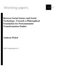
The environmental risk assessment of substances occurs through three main phases. The first phase
called pre-screening and prioritization provides a means for triaging substances so that they may be
prioritized for further assessment. The second phase, called the assessment phase, involves
-6-

characterizing the environmental exposure of a substance and the potential effects of a substance to
non-human biota. The final phase is the risk characterization phase and it involves determining the
risk potential of a substance according to a weight of evidence for exposure and effects. Throughout
the Environmental Risk Assessment (ERA) process, data are collected to support the assessment as
needed. Most data are collected during the pre-screening and prioritization phase and the assessment
phase. Dialogue with interested parties (e.g., regulatory managers, industry, and public) is also
conducted throughout the ERA as needed and may result in the re-iteration of an ERA as a result
of new ideas or data. Figure 2 provides an overview of the process for conducting the ERA of
substances.
2.3.1 Pre-screening and prioritization phase
The pre-screening and prioritization phase provides an initial first impression of the potential
concern a new or existing substance may pose to the environment. The intent of this stage is to
provide a rapid initial evaluation of a substance based on specific properties of the substance (e.g.,
persistence, bioaccumulation and toxicity) as well as information on the use, import/manufacture
volume, how the substance may enter the environment and the multi-media fate of the compound.
The results of pre-screening and prioritization can also be used to help set out a plan for the ERA
of a substance.
The level of detail of pre-screening and prioritization may vary between substances depending on
programs needs and the level of information available for a substance. For example, the
pre-screening of new substances is largely based on examination of a chemical’s structure, key
chemical properties, import/manufacture volume and intended use. This information is combined
to give an overall qualitative assessment of the priority of the new substance. For existing
substances, a scoring procedure involving several parameters may be used to provide a sequential
method of determining the priority of a substance for assessment. Regardless of the level of detail
of the pre-screening and prioritization a dialogue among risk assessors and managers is undertaken
to ensure that there is consensus on which substances are a priority.
2.3.2 Environmental fate phase
Once a substance is released to the environment from an anthropogenic activity, it becomes
important to understand where a substance will reside in the environment, how much of it will reside
there and for how long. Along with knowledge of how a substance enters the environment (i.e.,
mode-of-entry), how much and how often, understanding the environmental fate allows an assessor
to understand which environmental compartments are expected to contain the substance and
consequently which organisms may be exposed. Key physical-chemical properties of a substance
can be used to help determine environment fate (e.g., organic carbon partitioning coefficient, Henry's
Law Constant, bioconcentration factor, degradation half-lives). These properties can be entered into
a multimedia model to provide a better understanding of the partitioning behaviour of a substance
within and between environmental compartments and the overall residence time in a compartment.
-7-

Dialogue with Interested Parties (Managers, Industry, Public)
Prescreening and
Prioritization Phase
Environmental Fate
Assessment Phase
Characterization of
Characterization of
Exposure
Ecological Effects
Risk Characterization Phase
Collect and Generate Data / Reiterate Process as Needed
Figure 2: Framework for Conducting the Environmental Risk Assessment (ERA) of New and
Existing Substances
2.3.3 Assessment phase
The assessment phase consists of two main parts characterization of exposure and characterization
of ecological effects.
Exposure assessment characterizes the potential contact or co-occurrence of stressors (in this case
chemicals) with receptors (non-human target biota). Travis et al. (1983, cited in Barnthouse et al.
1986) defines exposure assessment for toxic chemicals as the “determination of the toxic materials
in space and time at the interface with target populations”. This is a very broad definition, but is
nevertheless important because it implies that the goal of exposure assessment is the determination
of a chemical concentration(s) in the environment that is considered toxic or presents a risk to
non-human biota. Extrapolating from this definition, it can also be held that regardless of how
inherently toxic a chemical can be, without organism exposure, there is no risk. Generally, estimates
of exposure are conservative and are based on reasonable worst-case scenarios that err on the side
-8-

of caution. The principles of pollution prevention under CEPA are implemented in the exposure
assessment by examining all reasonably anticipated future uses and related exposures.
Effects assessment characterizes the type and magnitude of ecological effects resulting from
environmental exposure to a chemical or a combination of chemicals. Often, in risk assessments, the
most sensitive receptor is used as the baseline from which to determine potential hazards to more
than one species. Often the type and magnitude of ecological effects is determined based on
measurement endpoints (e.g., median lethal concentration, median effects concentration for
reproduction). These endpoints correlate to the protection goals for the assessment (referred to as
assessment endpoints) and are used to evaluate potential threats to populations of species in the
environment. Ultimately, the effects assessment aims to derive the concentration of a substance in
the environment at which no effects are observable in target biota.
During the assessment phase, experimental and predicted data are collected or generated using
QSARs or environmental models. A re-iteration of the exposure or effects assessment may be
undertaken if there is sufficient concern for the substance or new data have been supplied or
collected. As with the pre-screening and prioritization phase, dialogue with interested parties (e.g.,
other assessors, managers, industry) is also performed to ensure that the characterization of exposure
and ecological effects is based on the best available information.
2.3.4 Risk characterization
The risk characterization phase brings together the information from the exposure assessment and
effects assessment with the aim of concluding whether a substance poses a risk to non-human biota.
The potential risk of a substance can be estimated using simple approaches such as the quotient
method or can be based on several lines of evidence (e.g., PBT properties of a substance) for both
biotic and abiotic endpoints.
The risk characterization phase also includes a qualitative assessment of the potential risk a
substance poses to the environment and will reach a conclusion on the toxicity of a substance as
defined under CEPA.
The risk characterization phase also points out where data gaps and uncertainties exist in the
assessment and how these factors impact the quality of the assessment. A re-iteration of the
assessment may be undertaken
2.4 The Need for a Multimedia Approach to Environmental Fate in ERA
In recent years, the characterization of uncertainty in ecological risk assessment has received much
attention and has become increasingly important regardless of the level of assessment performed.
Tools for characterizing uncertainty range from relatively simple qualitative approaches to complex
probabilistic designs. The ecological risk assessment of new substances in Canada uses a screening
level approach. Characterization of uncertainty at the screening level becomes very important
because typically fewer data are available and used to estimate risk.
-9-

In 1998 and 1999 the New Substances Division of Environment Canada undertook two studies to
examine qualitatively the uncertainties associated with the exposure assessment of new substances
in Canada (BEC 1999a; BEC 1999b). In the first study, a characterization of the data gaps and short
comings of the aquatic driven exposure assessment process was conducted. Specifically, a
characterization of the uncertainties associated with: (1) the estimation of release concentration, (2)
fate and distribution, and (3) release, fate and distribution in non aquatic media was described. One
of the key recommendations from the first study was that a multi media approach to conducting the
exposure assessment of new substances in Canada was needed in order to address releases to media
other than the water column. Although water column release and exposure form the basis for
determining the predicted environmental concentration of a new substance, releases to other media
do occur and are appropriate (e.g., accumulation in soils) but are not routinely considered. In the
second study, a strategy for dealing with the key data gaps and short comings that contribute to
exposure uncertainty was detailed. In this study a preliminary approach to conducting the multi
media exposure assessment (MMEA) of new substances was outlined.
The New and Existing Substances Branches of Environment Canada have acted on the MMEA
recommendation and strategy, which ultimately, led to the development of guidance for MMEA of
substances under CEPA (BEC 2001). Since 2001 many new multimedia tools and approaches have
been developed. In particular, as the Existing Substances Program embarks on the risk assessment
of substances categorized as persistent or bioaccumulative and inherently toxic, Environment
Canada recognized the need for up to date and detailed guidance on multimedia models and their
use in risk assessment. The result is this guidance document which is intended to be a evolving piece
of work that will be updated periodically as new techniques and understanding develop in the unit
world.
2.5 Practices in Other Jurisdictions
Practices in the US are generally similar to those in Canada in a scientific sense but the legislative
framework, the Toxic Substances Control Act, is different. Reference should be made to the USEPA,
Office of Prevention, Pesticides and Toxic Substances for guidance on current practices.
Chemical assessment in Europe is conducted by the European Chemicals Bureau (ECB) located in
Ispra, Italy. This organization collects information on chemicals used in Europe and prepares
priority lists. Priority substances are then allocated for assessment to specific member nations of the
European Union. Assessment reports are published and make recommendations on whether or not
some regulatory activity is deemed desirable. In recent years emphasis has been on “high production
volume” chemicals. It is suggested that the reader consult the ECB website (http://ecb.jrc.it) for
details of the assessment process (EUSES), priority lists, and technical guidance documents. The
assessment relies on the “SimpleBox” model developed by RIVM in the Netherlands.
Other national and international agencies also conduct assessments and provide guidance on model
use, notably Japan, the OECD, and UNEP.
-10-

3 MODELS AS A CONTRIBUTION TO UNDERSTANDING ENVIRONMENTAL FATE
3.1 What models can do for you
When seeking to understand the behaviour of chemicals in the environment, there is a consensus that
it is no longer satisfactory to begin production and discharge before having some degree of
assurance of the absence of risk. This has been learned from the tragedies of the past as highlighted
so elegantly by Rachel Carson (1962) in her book “Silent Spring”. Models provide a fast and
inexpensive mechanism for bringing together the best of current science on chemical fate processes
in the environment, with chemical properties data collected in the laboratory setting or from QSARs.
This should not be seen as excluding monitoring of in-use chemicals. For in-use and historic-use
chemicals, monitoring and modelling should play complementary roles. In the modelling context,
monitoring is critical for the continuing evaluation and improvement of the science on which the
models are based. Monitoring, in turn, benefits from the insights provided by modelling. Monitoring
programs contribute to the scientific understanding of environmental processes; better models are
developed; all with the ultimate benefit of improved chemical management.
As focus shifts from those substances already identified as problematic to a more preventive and
protective role, the weaknesses of existing science in explaining chemical behaviour become
evident. For example, the models which have long been used for such substances as PCBs may not
adequately describe fluorinated substances.
Historically, monitoring and modelling have primarily been conducted for the more populated
regions of North America and Europe. As global concern shifts from the immediate surroundings
of these affluent regions to the third world as a potential source and the polar regions as potential
destinations for contaminants, new environmental processes become important. The effects of
temperature, snow fall, and ice cover require improved representation within the models. Monitoring
and laboratory studies are required to facilitate the quantification of cold climate processes.
There are two fundamentally different types of models used in understanding chemical fate. The first
are statistical, knowledge-based models or correlations such as those contained in the EPIWIN suite
where similarities in properties imply similarities in behaviour. The second are mechanistic, processbased
models. Nearly all of the models developed by the CEMN are process-based models of
chemical fate.
Process-based models are a convenient way of bringing together the existing science in a simple
format to calculate expected chemical behaviour. Models need to be continually tested for validity
and challenged by monitoring programs and updated as the science existing at the time of model
development is shown to be inadequate for emerging chemicals or emerging concerns.
The models of the CEMN are founded upon the fundamental law that mass is neither created nor
destroyed, and therefore, these models are known as “mass balance models”.
-11-

A mass balance environmental model can:
i) reveal likely relative concentrations, i.e., it is useful for monitoring purposes by indicating
likely relative concentrations between media such as air, water, and fish.
ii)
iii)
iv)
show the relative importance of loss processes, i.e., the process rates that we need to know
most accurately
link loadings to concentrations, i.e., identify key sources and ultimately their effects
enable time responses to be estimated, i.e., how long recovery will take
v) generally demonstrate an adequate scientific knowledge of the system
Models are often not necessary when the sources, fate and effect are obvious, but they become more
valuable as situations become more complex, subtle, and with multiple sources. The user can also
play “sensitivity games” to determine what is most important and what is less important.
Models of the type described in this report can be used for the following general purposes.
i) to maximize our understanding of a monitored system.
ii)
iii)
iv)
to obtain the best possible understanding of the likely behaviour of a substance not yet being
monitored or not yet in production.
to enhance a monitoring program by providing guidance on the likely behaviour of the
substance of interest.
to evaluate the results of a monitoring program and test for any systematic error in the
chemical analysis, e.g., mis-reported units.
3.2 Environmental processes and pathways
There are three environmental processes or pathways to be considered in a mass balance model;
transformation or degradation processes, advection processes that move the chemical out of the
modelled system, and exchange processes between environmental media or compartments.
3.2.1 Transformation
A substance can be effectively removed from consideration by being transformed through a
chemical reaction. This is often described as degradation and first-order reaction kinetics are
assumed in analogy with radioactive decay. These reactions include photolysis, oxidation,
hydrolysis, and biodegradation.
-12-

Cautionary note:
Our focus here is on the degradation of the original or “parent” chemical. The
“daughter” product of any degradation reaction may or may not be more persistent,
bioaccumulative, or toxic than the parent substance and thus may merit further
investigation.
3.2.2 Advection
Advection processes such as wind transport and river currents can effectively remove a substance
from the modelled system by transporting it to a different location.
Cautionary note:
The substance may be more or less of a problem in the new location and thus may merit
further investigation.
3.2.3 Intermedia exchange
Exchange between environmental media can occur by a multitude of processes including diffusion,
rain dissolution, wet and dry aerosol deposition, runoff, and sedimentation and resuspension.
Depending on the specific model other processes may be included. The importance of each process
is highly dependent upon the chemical being investigated.
3.3 Fugacity concept
3.3.1 Origins, meaning, and usefulness
Fugacity was introduced by G.N. Lewis in 1901 as a criterion of equilibrium. It is similar to
chemical potential, but unlike chemical potential, it is proportional to concentration.
Fugacity, which means escaping or fleeing tendency, has units of pressure and can be viewed as the
partial pressure which a chemical exerts as it attempts to escape from one phase and migrate to
another. In many respects, fugacity plays the same role as temperature in describing the heat
equilibrium status of phases and in revealing the direction of heat transfer.
The application of the fugacity concept to environmental models is fully described in the text by
Mackay (2001).
When equilibrium is achieved a chemical reaches a common fugacity in all phases. For example,
when the fugacity of benzene in water is equal to its fugacity in air, we may conclude that
equilibrium exists. However, these common fugacities will correspond to quite different
concentrations. If the fugacity in water exceeds that in the air, benzene will evaporate until a new
equilibrium is established.
-13-

The use of fugacity instead of concentration thus immediately reveals the equilibrium status of a
chemical between phases and the likely direction of diffusive transfer. Further, the magnitude of the
fugacity difference controls the rate of transfer, by for example evaporation.
The relationship between fugacity (f, Pa) and concentration (C, mol/m 3 ) is given mathematically in
equation (1)
C = Zf (1)
where Z is a “fugacity capacity” or Z value with units of mol/m 3 APa.
When performing fugacity calculations, the SI units of mol/m 3 are used for all concentrations. It is
therefore necessary to convert from mg/L for concentrations in water, or mg/kg or :g/g for
concentrations in solid phases. A knowledge of the density (kg/m 3 ) of the solid phases is required.
3.3.2 Defining Z values
A Z value expresses the capacity of a phase, or environmental medium, for a given chemical. Z
values are large when the chemical is readily soluble in a phase, i.e., the phase can absorb a large
quantity of the chemical. A low Z value indicates that the phase can accept only a small quantity of
chemical, i.e., the chemical is “less-soluble” in the phase.
To establish Z values for each chemical in each phase, the process usually starts in the air phase. In
the air, the Ideal Gas Law is applied.
PV = nRT (2)
where P is pressure, or fugacity in our case, V is the volume of the air, n is the number of moles of
the chemical, R is the gas constant (8.314 PaAm 3 /molAK), and T is absolute temperature (K). Since
C = n / V, and C = Zf equation 2 can be re-written in fugacity terms as
Z A = 1/RT = C A /f A (3)
the subscript A referring to the air phase. Z A is thus about 0.0004 mol/m 3 APa for all chemicals in air.
A partition coefficient is the ratio of the concentrations in two environmental media at equilibrium,
thus it is the ratio of the Z values of the two media. For example, the air-water partition coefficient,
K AW , is
K AW = C A / C W (4)
= Z A f A / Z W f W
and since K AW is measured when f A equals f W , i.e., at equilibrium,
-14-

K AW = Z A / Z W (5)
In general,
K i,j = Z i / Z j (6)
Using the partition coefficients and previously calculated Z values, it is thus possible to calculate
Z values for the chemical in other media such as soil, fish, and sediment if dimensionless partition
coefficients are known.
Cautionary Note:
Care must be taken to ensure that the partition coefficients are dimensionless because
many are reported in dimensional units such as L/kg, i.e., a ratio of a solid phase
concentration (mg/kg) to a liquid phase concentration (mg/L). The preferred units of
both concentrations when calculating partition coefficients are mol/m 3 or g/m 3 . This
ensures that the partition coefficient is dimensionless.
A very convenient and important description of chemical hydrophobicity or lipophilicity is K OW , the
octanol-water partition coefficient, which is the ratio of Z in octanol to Z in water. Octanol is
commonly used as a surrogate for lipids and organic matter in the environment. Hydrophobic
chemicals such as DDT or PCBs have K OW values of about a million implying that Z O is about a
million times Z W , i.e., the water phase has a very limited capacity for the chemical. The chemical
is thus “water hating” or hydrophobic. K OW is used in correlations to describe partitioning from
water into lipids of fish and other organisms and into natural organic carbon such as humic material.
It is also used to correlate toxicity data for a variety of chemicals.
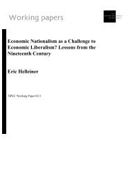
Correlations have been developed for several partition coefficients for organic chemicals as a
function of chemical properties such as solubility in water, K OW and vapour pressure. These can be
exploited to give “recipes” for Z values. Caution must be exercised when using these correlations
for chemicals of unusual properties such as ionizing acids or bases, detergents, dyes and polymers.
Figure 3 is a summary of expressions which can be used to estimate Z values, detailed justification
being given in Mackay (2001). Notable is the use of K OW to estimate K OC the organic carbon
partition coefficient which is the key to the estimation of soil-water and sediment-water partition
coefficients for many compounds.
Pure solutes are rarely present in the environment except as a result of chemical spills. The Z value
for a pure solute is thus of more academic than practical interest. The fugacity of a pure solute is its
vapour pressure, P S (Pa). The concentration (mol/m 3 ) is the reciprocal of the molar volume, v
(m 3 /mol). It follows that Z is 1/(P S v).
-15-

C O
OCTANOL
C B
BIOTA
C A
AIR
VAPOUR PRESSURE
P S v/RT
C P
PURE
Z A
= 1/RT
SOLUTE
Z O
= K OW
/H
Z P
= 1/P S v
f
FUGACITY
Z S
= K B
ρ B
/H
Z S
= K P
ρ S
/H
Z W
= 1/H
= C S /P S C
BIOCONCENTRATION SORPTION S
FACTOR
COEFFICIENT SORBED
ρ B
K B
K OW
OCTANOL-WATER
PARTITION COEFF.
C W
WATER
ρ S
K P
C S v
AQUEOUS
SOLUBILITY
AIR-WATER PARTITION COEFF.
H/RT or P S /RTC S or K AW
Compartment
Definition of Fugacity Capacities
Definition of Z, mol/m 3 Pa
Air 1/RT R = 8.314 Pa m 3 / mol K T = temperature, K
Water 1/H or C S /P S H = Henry’s law constant, Pa m 3 / mol
C S = aqueous solubility, mol/m 3
P S = vapour pressure, Pa
Solid Sorbent (e.g. soil,
sediment, particles)
K P D S / H
K P = solid-water partition coefficient, L/kg
D S = density of solid, kg/L
Biota K B D B / H K B = biota-water partition coefficient, L/kg or
bioconcentration factor (BCF), L/kg
D B = density of biota, kg/L (often assumed to be 1.0 kg/L)
Pure Solute 1 / P S v v = solute molar volume, m 3 /mol
Figure 3: Relationships between Z values and partition coefficients and summary of Z value
definitions.
-16-

3.4 An exploration of Levels
It is useful to explore the behaviour of a chemical in the environment through a series of models of
increasing complexity. The simpler models are easiest to understand and have fewest data
requirements. As the complexity of the models increase, they become more challenging to
understand and the data requirements increase. When more input data must be estimated, the
reliability of the model output may become compromised. By stepping through a series of models
of increasing complexity, understanding of the chemical’s behaviour can be maximized while the
likelihood of gross mis-representation is minimized.
Here the assumptions for the four levels of complexity are described. These calculations are
embodied in a set of model software, each named for the level it contains, and in other software for
specific purposes. The software is described later.
3.4.1 Level I: simple equilibrium partitioning calculations
It is simplest to begin by assuming a closed environment with a constant amount of chemical present
at equilibrium between the environmental media. This “pop can” environment has no mechanisms
for chemical to be added or removed. There are no degradation or advection processes. There is no
active transport between environmental media; to return to the heat capacity analogy used
previously, the can has been on the shelf for long enough to have reached a constant temperature.
In fugacity terms, this assumption of equilibrium means that a single fugacity exists in the
environment, i.e., in a four-compartment environment where A is air, W is water, E is soil or “earth”,
and S is sediment,
f A = f W = f E = f S = f (7)
A Level I model combines chemical partitioning (measured or estimated) data to give the Z values
in each medium in the environment and, more importantly, the chemical’s partitioning tendency. The
inter-media surface areas are not needed because equilibrium is assumed between well-mixed
volumes of media.
The partitioning behaviour of a chemical can be most readily depicted and understood with a
chemical space diagram such as that shown later in Figure 4.
Some algebra
M is total moles of chemical in the environment, V i is volume, and C i is concentration for
compartment i and all summations are over all i.
M = GV i C i = GV i Z i f i (8)
and since all f i are equal and can be designated f by equation (7)
M = f GV i Z i (9)
-17-

or
f = M / GV i Z i (10)
This is a Level I calculation.
The calculation sequence is
• given the partition coefficients of a chemical, Z values can be determined
• given compartment volumes, Z i V i can be determined
• given an amount of chemical present, f can be determined from equation (10), and
• from f, all concentrations, C i = Z i f and all amounts m i = C i /V i can be determined.
As a final check, the sum of all m i must equal the total amount of chemical present.
A simple worked example for DDT in a water body such as a lake is given in Appendix D.
3.4.2 Level II: equilibrium partitioning with loss processes
The modelled complexity of the environment at equilibrium can be increased by including the loss
processes of advection and degradation. Advection includes mechanical removal processes such
achieved by air and water currents and is characterized by a flow rate, G (m 3 /h). Degrading reactions
can include both chemical reactions and biologically-mediated degradation, and are characterized
by a half-life, J (h) or rate constant, k (1/h) = ln(2) / J. A set of transport or transformation values
known as fugacity rate constants or D values ( mol / Pa h ) are calculated as D = G Z or D = k V Z
where V (m 3 ) is the volume of the medium. Since the equilibrium assumption is maintained in Level
II calculations, there is no dependence on the medium to which the chemical is emitted; and total
emission into the environment is sufficient to describe chemical entry to this system. Again, the
inter-media surface areas are not needed as equilibrium is assumed between well-mixed volumes
of media.
Some algebra
E is emission rate in mol/h
and by equation (7) and re-arranging equation (11)
This is a Level II calculation.
E = GD i f i (11)
f = E / GD i (12)
The calculation sequence is
• use the Z values from Level I
• given compartment volumes, rate constants, and flow rates, all D i values can be determined
• for advection processes, A: D iA = G i Z i
-18-

• for reaction processes, R: D iR = k i V i Z i
• given an emission rate, f can be determined from equation (12), and
• from f, all concentrations, C i = Z i f and all rates D i f can be determined.
As a final check, the sum of all loss rates D i f must equal the emission rate.
A simple worked example of DDT in a water body is given in Appendix E.
3.4.3 Level III: steady-state with multimedia transport
By removing the equilibrium assumption, the model complexity and data demands are again
increased. The steady-state assumption, i.e., the absence of change over time, is retained. Without
the equilibrium assumption the chemical’s fugacities in each medium generally differ and, it is now
necessary to describe active transport processes between environmental media. These can include
processes such as diffusion, volatilization, deposition, resuspension, and runoff and require a variety
of input data depending on the details of the environment modelled. For example, media volumes
are no longer sufficient. The inter-media surface areas are needed to calculate many of these transfer
process rates. In general, D = A U Z where U is the transport velocity for the process in units of m/h
and A is the area of the exchange surface in m 2 . Medium-specific emission rates, E i , are now
required because the results are strongly dependent on the receiving medium or media, i.e., the
“mode-of-entry”. This more complicated calculation will yield the same results as a Level II
calculation if the chemical is rapidly transported between media such that all media have the same
fugacity - the key assumption of Level II.
Some algebra
Ei are the emissions into each medium i, D i,j are the fugacity rate constants for chemical transfer
from medium i to medium j. Since chemical mass is conserved, the amount entering each medium
must equal the amount removed by either transport into another medium or by one of the loss
processes of advection and degradation.
Losses in medium i are given by
Entering = Advected + Degraded + Transferred (13)
D iT = D iA + D iR + GD i,j (14)
E i + GD j,i f j = f i D iT (15)
Note that GD j,i f j is the sum of the rate of input from other compartments j to compartment i.
Re-arranging equation (15) gives
f i = ( E i + GD j,i f j ) / D iT (16)
We thus obtain for n media, n equations with n unknown fugacities and we can solve them for all
fugacities, from which concentrations, amounts and rates are calculated.
-19-

Note that we can have as many boxes as we like - the limitation is our ability to estimate D values,
not computing power.
This is a Level III calculation.
The calculation sequence is
• obtain the Z values from Level I, and D iA and D iR from Level II
• given the necessary transfer process information, calculate all D i,j
• given all emissions, Ei, the set of mass balance equations (16) will yield the set of fugacities,
and
• from all f i , all concentrations, C i = Z i f and the total removal rate from the environment
G(D iA f i + D iR f i ) can be determined.
As a final check, the total removal rate must equal the sum of the emission rates, GE i and each
compartment should also display a mass balance with inputs equalling outputs.
A simple worked example for DDT in a water body is given in Appendix F.
3.4.4 Level VI: dynamic
This next level of complexity, Level IV, includes change over time, i.e., it does not assume steadystate.
Here a single emission such as a spill may be followed through time, or the effect of emission
reductions examined in detail. Sufficient input data is often difficult to obtain and erroneous
estimates can lead to false conclusions. Thus, it is important to follow a progression of increasing
model complexity and data demands to anticipate the likely dynamic behaviour prior to performing
such calculations.
Some algebra and some calculus
For a time-varying emission to medium i, E i (t), mass balance dictates that all chemical entering
medium i must be accounted for through transport into another medium or by one of the loss
processes of advection and degradation or must become a part of the inventory of chemical in
medium i. Thus the amount of chemical in medium i at time t is given by
m i (t) = m i (t-1) + )t dm i /dt (17)
dm i /dt = d(f i V i Z i )/dt = rate of chemical entering - rate of chemical leaving (18)
or assuming volumes and Z values are constant
V i Z i df i /dt = E i (t) + GD j,i (t) f j (t) - f i (t) D iT (t) (19)
In equation (19) the left-hand side is the inventory change and the terms on the right-hand side are
direct emission to the compartment, transport to the compartment, and losses from the compartment.
-20-

D iT it the total of all loss D values by reaction, advection, and intermedia transport. A dynamic
calculation for constant emissions, if continued for a long enough period, will achieve the steadystate
condition and results will be equivalent to those from the Level III calculation.
There are thus n simultaneous linear differential equations. They can be solved analytically but it
is often easier to solve them by numerical integration. The result is the time-course of concentrations
in each medium.
3.4.5 Summary of Levels
Table 1: Summary of Levels of complexity in multimedia models
Level Assumptions
I
II
III
VI
Closed system
Defined chemical amount
Equilibrium between media ==> one fugacity
Single chemical emission rate
Reaction and advective loss processes
Equilibrium between media ==> one fugacity
Chemical emission rates and mode-of-entry
Reaction and advective loss processes
Non-equilibrium between media ==> different fugacities
Steady-state system, i.e., unchanging with time
Dynamic system, i.e., changing with time
3.5 A Six-Stage Process to Understanding Chemical Fate
In 1996, Mackay et al (1996a) outlined a 5-stage process to understand the behaviour of a substance
in the environment. The five stages are: (1) chemical classification, (2) acquisition of discharge data,
(3) evaluative assessment of chemical fate, (4) regional or far-field evaluation, and (5) local or nearfield
evaluation. A sixth stage was suggested by MacLeod and Mackay (1999) in which an exposure
evaluation would be conducted.
Recently, in recognition of the challenges of obtaining the emission data for stage 2, it has been
suggested that target emissions can be calculated from critical concentrations to evaluate risk. A
more detailed discussion of this risk evaluation is given later.
This process generates an increasing understanding of the chemical of interest. Often sufficient
information will be generated early in the process and the final stages will be unnecessary, or allow
simplifying assumptions to be made without loss of accuracy. For example, when gathering the data
for stage 1, it may become evident that the substance is not multimedia in nature but partitions
-21-

exclusively to only one or two environmental media. In such a case, the degradation half-lives in the
media to which it does not partition may be assumed to be infinite (i.e., the rate is zero) and do not
need to be measured or estimated.
This gradual increase in data requirements and complexity facilitates the mental assimilation of the
information generated. By plotting the partitioning properties of a substance much may be learned.
By calculating the substance’s fate in an evaluative environment, key processes can be identified.
It is argued by some that all the information may be generated by using a single, complex and
realistic model. This assumes that all of the required input data are available. It assumes that all the
process information encoded in the model is correct and applicable. It assumes that the greatest
realism is always required and that the results will always be interpretable.
It is well-established that as models increase in realism and complexity, the data demands increase;
data demands that are often impossible to satisfy except through estimation methods. As more input
data are estimated, the reliability of the results becomes compromised. Also, as the complexity of
the model increases, the results become more challenging to interpret and thus more prone to misinterpretation.
For these reasons, we recommend that simpler models be applied first and the complex models only
used when necessary.
Occam's razor or the Principle of Parsimony
Essentia non sunt multiplicanda praeter necessitatem
"What can be done with fewer (assumptions) is done in vain with more"
3.5.1 Stage 1: Chemical classification and physical data collection
Partitioning
For convenience in modelling, three chemical types have been defined (Mackay et al, 1996a). this
allows these chemicals to be treated by multimedia models such as those developed by the CEMN.
The defining characteristics and some examples are given in Table 2. Table 3 gives the typical
property data required for a chemical of each defined type. Data sources and estimation methods are
suggested later in this section.
-22-

Table 2: Chemical types are based on partitioning behaviour.
Type Partitions
into
Z
Equilibrium
criterion
Examples
1 all media non-zero in
all media
2 not air . or = 0 in
air
3 not water . or = 0 in
water
fugacity
aquivalence
fugacity
most organic chemicals (e.g.,
chlorobenzenes, PCBs) including
ionizing chemicals
cations, anions, involatile organic
chemicals, and surfactants
very hydrophobic compounds (eg.,
long-chain hydrocarbons, silicones)
4 not air and
not water
. or = 0 in
air and water
none
polymers
5 speciating chemicals (e.g., mercury)
Type 4 substances tend to remain in their original state as a solid in the environment thus modelling
of the type described in this document does not serve a useful purpose. It should be noted that
polymers may contain unreacted monomer and other additives such as plasticisers that are of
possible concern. These substances may degrade to form other chemicals that can have adverse
effects.
Type 5 substances display complex environmental fate and require case-specific evaluation.
Table 3: Typical physical chemical property data required for each chemical type
Type Data required
1 molar mass, data collection temperature, solubility in water, vapour pressure, and
octanol-water partition coefficient (K OW ) and possibly pK a
2 partition coefficients from solids or organic carbon to water
3 partition coefficients from solids or a pure phase to air
Aquivalence
The Z values for Type 2 chemicals are calculated using the aquivalence approach (Mackay 2001).
Since the vapour pressure and the air-water partition coefficient may be zero, Z for water becomes
infinite if calculated as for Type 1. Therefore, calculation starts by defining Z for water as 1.0. All
other Z values are deduced from the Z value for water and the partition coefficient of the phase with
respect to water.
-23-

Ionizing Chemicals
Organic acids and bases such as phenols, carboxylic acids, and amines, may dissociate or ionize in
the environment. As a result of this tendency to dissociate an acidic substance may exist in its nonionic
protonated or neutral form and its ionic de-protonated, or charged, form. Bases behave
similarly but the protonated form is charged. These forms have different properties, for example the
neutral form may evaporate from water, but the ionic form does not evaporate. It is thus essential
to calculate the fractions in each form.
The simple, first order approach of Shiu et al (1994) and Mackay et al (2000) to quantifying these
fractions is briefly described below.
The neutral form of an acid molecule can be designated RH where R is an organic molecule
comprising carbon, oxygen, hydrogen and possibly sulfur, nitrogen and phosphorus. When dissolved
in water, the molecule may ionize to form hydrogen ion H + and an anion R -
RH 6 R - + H +
The molecule may have several hydrogens that can dissociate. No correction is made for the effect
of cations other than H + . It is assumed that dissociation takes place only in aqueous solution, not in
air, organic carbon, octanol or lipid phases. Some ions and ion pairs are known to exist in the latter
two phases, but there are insufficient data to suggest a general procedure for estimating quantities.
The dissociation constant is defined as follows.
Ka = [R - ] [H + ] / [RH] (20)
so
pKa = log ([R - ] [H + ] / [RH]) (21)
Typical values of pKa for chlorinated phenols range from 4 to 8. It is the relative magnitudes of pKa
and pH, the environmental acidity, that determine the extent of dissociation.
Rearranging equation (20) gives
log ( [R - ] / [RH] ) = log I = - log [H + ] + log Ka (22)
= pH - pKa
where I is the ratio of the ionized to non-ionized concentrations, pH is -log [H + ] and pKa is -log Ka.
Note that base 10 logarithms are used. This leads to the Henderson Hasselbalch equation
I = 10 (pH - pKa) (23)
Note that if the substance has several pKa values, the one corresponding to the primary or first
dissociation process should be used. This has the lowest value of pKa. For example, if values of 5,
8 and 11 are given, use 5 and ignore the others, at least for screening purposes.
-24-

Assuming a pH of 7.0 and that the ionic form does not evaporate from water, sorb to organic matter,
or bioaccumulate into lipids, this ratio is assumed to apply in all water phases in the environment.
As a result of ionization, there can be ambiguity about the values of the solubility in water and K OW .
If experimental data are used, the pH should also have been specified to clarify if the properties are
those of the non-ionised or non-ionised plus ionised forms. If the latter applies, the solubility and
K OW of the non-ionised form can be calculated. If the data are from an estimation method, the values
generated will correspond to the molecular structure provided to the method. For example, a
SMILES notation used in QSARs will normally refer to the non-ionised form, not the ionised form
Models treating ionizing chemicals normally require the solubility of neutral species either from an
estimation method or measured.
For the general case of a pKa measured at an acidity of pH d , where the subscript d represents the
data pH, the ionic to non-ionic ratio at of pH d is
thus the non-ionic fraction is
pHd
− pKa
I d
= 10 ( )
(24)
and the ionic fraction is
x
Nd
= 1/( 1+
I )
xI = Id /( 1 + I
d d)
d
(25)
(26)
The Z Td
for both species in water at the pH of the data collection is 1/H d , therefore the Z for the
ionic fraction is
Similarly the Z for the non-ionic fraction is
Z = x × Z
I I T
d d d
(27)
Z = x × Z
Nd Nd Td
(28)
But, the Z for the non-ionic fraction is unaffected by the pH of the water and therefore, at the pH of
the environment (e) is given by
Z = Z = x × Z
N N N T
e d d d
(29)
The Z for the ionic fraction, at the pH of the environment, is given by
Z
=
I Z
Ie
e Ne
(30)
And finally, the Z for both species together, at the pH of the environment, is
Z = Z + Z
Te Ne Ie
(31)
-25-

To calculate the D values for the loss and transfer processes care must be taken to use the Z value
relating to the species participating in the process.
The same arguments apply to bases. Rather than use the constant Kb it is usual to express it also as
Ka, noting that pKa + pKb = 14.
Note that in the Handbook by Mackay et al (2000) the aqueous solubilities selected are primarily
those of the non-ionic form.
Degradation
Chemical transformation, or degradation, can be considered to be the decomposition of the substance
of interest into water, carbon dioxide, and inorganic compounds, however, only primary degradation,
i.e., the degradation causing a change in the identity of the substance, is considered here. The
daughter compounds are normally considered separately from the parent compound as they have a
completely different set of properties, including a different toxicity, and thus a different priority.
Degradation is normally characterized as a first-order reaction and quantified by a reaction rate
constant, k i (1/h), or a half-life, J i (h) = ln(2)/k i in each environmental medium, i. Degradation occurs
by processes such as photolysis, hydrolysis, oxidation and biodegradation. The rates of these
processes are strongly dependent upon environmental conditions such as temperature, solar
insolation, and the nature and activity of the microbial community. Thus degradation data are
characterized by a high inherent variability. For a more detailed discussion of natural variation in
degradation half-lives consult Boethling and Mackay (2000) or Webster et al (1998). Various
researchers have sought to acknowledge this variability by defining degradation classes and
including a range of values in each class. For example, Syracuse Research Corporation (SRC), uses
an semi-quantitative scheme based on designations of hours (4.1 h) , hours to days (30 h), days (56
h), days to weeks (208 h), weeks (360 h), weeks to months (900 h), months (1440 h), and
“recalcitrant” (3600 h) ( ref ). Another is the lognormal classification scheme of Mackay et al (2000)
and Webster et al (2003) as shown in Table 4.
-26-

Table 4: Lognormal degradation classification scheme.
Class Mean half-life (hours) Range (hours)
1 5 11 years) > 100000
Cautionary note:
The absence of degradation gives an infinite half-life. In practical terms, this can be
represented by the very large half-life value of 10 11 hours which translates to a
negligible reaction rate. A half-life of zero, by contrast, indicates an infinitely fast
reaction process. Most CEMN models prohibit the unrealistic entry of a zero half-life.
Data sources and estimation methods
For chemicals that have been studied, there are some excellent compilations of data such as Mackay
et al (2000), Verschueren (2001), and the Handbook of Environmental Fate and Exposure Data for
Organics by Howard (1989, 1990, 1991, 1993, and 1997).
In the absence of data, estimation methods must be used to determine chemical partitioning
properties. These methods should be used with caution and with a knowledge of the limitations of
the method. A very brief overview is provided here. For more information, the reader is referred to
Boethling and Mackay (2000), and Mackay (2001). Some estimation methods are included in the
EPI Suite software (available from http://www.syrres.com/esc/est_soft.htm or
http://www.epa.gov/oppt/exposure/docs/episuitedl.htm).
Henry’s Law Constant, H (Pa m 3 /mol)
The air-water partition coefficient, K AW , is H / RT where R is the gas constant, 8.314 Pa/m 3 , T is
temperature (K), and H can be estimated from the vapour pressure, P (Pa), and the water solubility,
S (mol/m 3 ), (Mackay 2001). Note that both P and S must be of the same state, i.e., solid (S) or liquid
-27-

(L). That is, H = P L / S L or H = P S /S S . For substances with a melting point greater than 25 /C, i.e.,
solids at room temperature, a fugacity ratio, F, can be defined from the melting point, MP, and the
temperature at which P S was measured (normally about 25 /C).
F = e (6.79 x (1-MP/T) (32)
The sub-cooled liquid vapour pressure, P SL is then P S / F and H = P SL / S L
Organic Carbon Partition Coefficient, K OC (L/kg)
The organic carbon - water partition coefficient, K OC (L/kg), can be estimated from either K OW , or
the water solubility, S.
Table 5: K OC estimation methods
Estimation
Source
K OC (L/kg) = 0.41(kg/L) K OW Mackay 2001
K OC (L/kg) = 0.35(kg/L) K OW Seth et al 1999
equations of the form
log K OC = a log K OW + b
with various values of a and b
equations of the form
log K OC = a log S + b
with various values of a and b
Boethling and Mackay 2000
p153 Table 8.1
Boethling and Mackay 2000
p154 Table 8.2
Soil and Sediment - Water Partition Coefficients
The partitioning between the solid fraction of soil or sediment, and water, can be obtained as a
measured equilibrium partition coefficient, K p (L/kg) = C S (mg/kg) / C W (mg/L). Using the density
of the solids, a dimensionless partition coefficient can be determined. For example, for soil,
K Soil Solids, Water = K p (L/kg) D Soil Solids (kg/m 3 ) / (1000 L/m 3 ) (33)
where D Soil Solids is the density of soil solids and 1000 L/m 3 is a volumetric conversion.
It is also possible to estimate K p from K OC as
K p (L/kg) = y K OC (L/kg) (34)
where y is the mass fraction of organic carbon present in the soil solids (i.e., dry soil) (Boethling and
Mackay 2000; Mackay 2001). There are four assumptions that must apply to use this estimation
method, otherwise K d should not be estimated using this equation.
- 1 - sorption is exclusively to the organic component of the soil (or sediment)
- 2 - all soil (or sediment) organic carbon has the same sorption capacity per unit mass
- 3 - equilibrium is observed in the sorption-desorption process
- 4 - desorption isotherms are identical.
-28-

Aerosol - Air Partition Coefficient
Aerosol - air partitioning is not normally measured for evaluation purposes. It can be measured in
the environment by measuring concentrations in air before and after filtration. It is variously
estimated as shown in Table 6.
Table 6: K QA estimation methods
Estimation
Source
K QA = 6 x 10 6 / P L Mackay 2001
K p (m 3 /:g) / K OA = B where B is b × 10 -12 thus
K QA = K OA ×D Q (kg/m 3 ) × b × 10 -3 (m 3 /kg)
b is approximately 1.5 for most persistent organics
logK p = (a * logK OA ) + b or
K QA = K a OA ×D Q (kg/m 3 ) ×10 ( b + 9) (m 3 /kg)
a is approximately 0.55 and b is -8.23 for most persistent organics
log K P (m 3 /:g) = log K OA -12.61 or
K QA = K OA ×D Q (kg/m 3 ) × 10 -3.61 (m 3 /kg)
Finizio et al 1997
Finizio et al 1997
Bidleman and Harner,
2000
Due to the small volume of aerosols present, the amount of chemical sorbed is small. For substances
with a high K OA , the concentration may be high and scavenging may be an important transport vector
for removal of the substance from the air. For low K OA substances, partitioning to aerosols is
relatively unimportant. When K OA is very large, i.e., 10 10 and above, most chemical in the
atmosphere is likely to be sorbed to aerosols. Benzo[a]pyrene is an example.
Biota - Air and Biota - Water Partition Coefficients
Partitioning between the abiotic and biotic media in the environment is not normally measured.
Partitioning between biota (B) and the air or water is usually estimated assuming partitioning to only
the lipid fraction. If this assumption is not true, some other estimation method should be used. For
aquatic biota such as fish, if a lipid fraction of 0.05 is assumed, then the partitioning coefficient, K BW
= 0.05 K OW . Similarly for vegetation, if the leaves are assumed to have a lipid fraction of 0.01, the
leaf-air partition coefficient, K BA = 0.01 K OA . For roots, a root-water partition coefficient may be
estimated in the same way.
Degradation
As for chemical partitioning properties, there is a variety of data sources including those listed
above. Specific to degradation data is the Handbook of Environmental Degradation Rates (Howard,
1991). Estimation methods have also been developed. A review of existing methods and suggestions
for their application are given in a companion document to this report (Arnot et al, 2005). Some
estimation methods are included in the EPI Suite software
(http://www.epa.gov/opptintr/exposure/docs/episuite.htm).
-29-

Toxicity
It is important to identify the potential for concern regarding the toxicity of the substance. If a
substance is unlikely to have toxic effects at the expected concentrations, it may not warrant further
investigation. A substance with a higher probability of toxic effects should be investigated first, and
more fully.
To a first approximation there are three methods of expressing toxicity.
First is to define a concentration external to the organism that will cause a specified effect such as
lethality of failure to reproduce. The aquatic LC50 and the occupational Threshold Limit Value
(TLV) in air, applicable to occupational exposure, are examples.
Second is a dose, often expressed in mg/kg body weight per day, which causes an effect. This is
widely used in human toxicology. The dose may be the product of a concentration in food and the
quantity of food consumed per day.
Third is the delivered dose or the internal concentration or quantity or critical body residue of
chemical causing the effect. For example, a chemical that exerts toxicity by narcotic or baseline
toxicity does so at a concentration in the body of 1 to 5 mmol/kg body weight. The concentration
may also be in a specific tissue within the organism. Generally, chemicals which have similar modes
of toxic action have similar internal concentrations at the same effect level. Obviously the
calculation of this concentration requires a bioaccumulation or even a pharmacokinetic model.
The issue evaluating toxicity is beyond the scope of this Guidance but it is useful for the modeller
to know how the results are to be used in the evaluation of toxic effects. Many believe that the future
of environmental toxicology lies in calculating the third metric of toxicity, namely the critical body
residue required to cause the specified mode of toxic action. The mode of action can, in principle,
be predicted from molecular structure.
3.5.1 Stage 2: Acquisition of discharge data
This is typically a very challenging task. For many substances of concern, discharges are dispersed
and highly population and culturally dependent. The components of automobile exhaust are typical
of this group of substances. At the other extreme are substances discharged at point-sources, often
industrial in nature. Where such discharge data exist they may be incomplete or suited only localscale
evaluations.
-30-

3.5.2 Stage 3: Evaluative assessment of chemical fate
Armed with the data collected in stages 1 and 2 of this 6-stage process, modelling is now both
possible and useful. An examination of the behaviour of the substance in a generic or “evaluative”
environment increases our understanding without requiring regional properties and in a way that can
be compared across regulatory jurisdictions. This can be preformed with a models such as the 3-part
set Level I, Level II, Level III or the EQC model that combines the calculations of the other three
but with less flexibility for the user. (See Section 4.3.1 to 4.3.4 for details on these models.) For an
evaluative assessment a unit amount or rate of emission can be used as absolute concentrations are
not the focus of this stage of the six-stage process.
The area for an evaluative assessment should be large enough that wind dispersion does not
dominate the distribution of concentrations to the exclusion of all other information. In the EQC
model an area of 10 11 m 2 or10 5 km 2 . This is about the size of southern Ontario or twice the size of
Nova Scotia. This is large enough to show chemical exchange behaviour in the environment. If as
area on the order of a few kilometres square is used, local sources and wind patterns will dominate
and a dispersion model should be used. One can consider two extremes of scale, for very small areas
losses are entirely dominated by advection but for the entire globe degradation losses dominate.
Degradation and advection losses become equal when the reaction half-life is similar to the
advection residence time. The smaller value dominates since it reflects a faster process.
In the Level I calculations, the partitioning properties of a chemical are used to show the
environmental media in which it will tend to be present. The term “realistic presence” has been used
to designate an amount of at least 5% in an environmental medium (Webster et al 2004a; Woodfine
and Mackay 2001; Environment Canada 2003). A multimedia chemical is realistically present in
more than one environmental medium. For single-medium chemicals, i.e., chemicals with a realistic
presence in only one medium, multimedia models are neither needed nor useful. The fate of a singlemedium
chemical is limited to processes occurring solely in that medium (advection and
degradation). Multimedia models should only be used if the chemical is realistically present in at
least two environmental media.
The “realistic presence” concept has been suggested as a rational method of avoiding demands for
data which prove to be of little or no value. If a chemical is present only to the extent of say 2% in
a medium it is unlikely that the overall fate of the chemical, especially its persistence, will be
affected by rates of degradation in that medium. It can thus be argued that no degradation rate data
are needed and a zero degradation rate (infinite half-life) can be assumed. The 5% cut-off has been
established by experience but is somewhat arbitrary. (Woodfine and Mackay 2001, Webster et al
2004a).
In the Level II calculations, the partitioning and degradation properties of a chemical are combined
to give a first estimate of the relative importance of each removal process, and the longevity or
persistence (P) and long-range transport potential (LRT) of the chemical. While current Level II
models do not explicitly calculate LRT it can be calculated manually as the product of an assumed
wind speed (km/h), the overall residence time of the chemical (h), and the ratio of the amount in air
-31-

to the total amount in the system. The values of P and LRT should be considered in the context of
the values for ranking against other chemicals. The absolute value P and LRT calculated by these
models are not meaningful.
For multimedia chemicals that are not realistically present in at least two media as identified in the
Level I calculations, the same simplifying assumptions regarding the degradation data requirements
for Level II calculations may be made. For example, if a chemical does not partition appreciably into
air, the degradation half-life in air can be assumed to be infinite, i.e., assume no degradation of the
chemical in a medium in which it is not present. This assumption represents a reduction in the data
requirements while having a minimal impact on the model results (Woodfine and Mackay 2001,
Webster et al 2004a, Environment Canada 2003).
In a Level III calculation, the partitioning and degradation properties of the chemical are combined
with intermedia transport process information. In the absence of the equilibrium assumption, the
relative emission rates to each environmental medium becomes essential information because the
results are often strongly dependent on the mode-of-entry. It is common practice among researchers,
when these relative emission rates are not known, to perform a separate Level III calculation for a
unit emission into each potential receiving medium and focus on the worst-case scenario. Thus if
there are three potential receiving media, the calculations are performed three times, once for each
medium as receiving a unit emission. The results of the three scenarios are compared and the
assessor can then focus on the worst-case, e.g., the unit emission to air. Identifying the worst-case
scenario will require a knowledge of the target organism and exposure routes. Of course, if emission
mode-of-entry data are available they should be used.
From the Level III model and using the evaluative environment the relative importance of each
transport and removal process can be ascertained for the chemical and emission scenario under
investigation. The importance of each process is chemical and emission scenario dependent and can
not be determined in a general way. Consider for example, a chemical with a high K OA emitted to
air. This chemical will sorb strongly to aerosols and wet and dry aerosol deposition will be
important. Rain rate will be important as it affects the rain scavenging of this aerosol-associated
chemical. The dissolved fraction of the rain deposited fraction of chemical will be relatively less
important and depends on the K AW of the chemical.
Level III calculations also provide values for P and LRT. When the relative emission rates to each
environmental medium are known, this represents an improvement on the estimate provided by the
Level II calculations. It is not yet clear that there is any benefit from these estimates of P and LRT
where the relative emission rates are not known, at least with some degree of confidence. The value
of LRT is, again, not meaningful in an absolute sense but should be compared to the values for other
chemicals to provide a ranking. The value of P, while meaningful, may also usefully be compared
between chemicals.
Finally, Level III calculations using an evaluative environment can be compared to monitored
concentration data. This must be done with some care and acknowledging the inherent error that will
be caused by the properties of the evaluative environment not matching those of the region where
-32-

the data were collected. There are some advantages to this pseudo-regional modelling. First,
monitoring data from a variety of regions can be combined. For example, much of the northern US,
southern Canada, and western Europe all have somewhat similar environments. Thus when
monitoring data are sparse, data from all of these regions can be combined and the model results
compared to the range of monitored values. It is of particular interest to compare the relative
concentrations, that is, if the monitored concentration in the soil samples is ten times that of the
water samples, is this seen in the model results? This type of comparison may point to selective
sampling where only locations of high concentration need be monitored.
3.5.3 Stage 4: Regional or far-field evaluation
Regional or far-field evaluations with region-specific environmental properties provide the first set
of concentrations for direct comparison to monitoring data collected in a specified area such as
Southern Ontario, or Northern BC.
The ChemCAN model was developed for this purpose and contains a database of properties for 24
regions of Canada. For consistency and comparison the database also contains the standard EQC
environment.
As for an evaluative assessment, a region should be defined as an area large enough that wind
dispersion does not dominate to the exclusion of all other information. Local hot spots are not
treated. It is important when defining a region for this stage in the process to specify an area large
enough that advective flow-through will not dominate the chemical removal processes such that all
intermedia and degradation effects are obscured. In ChemCAN the Canadian regions range in size
from 2176000 km 2 for the Arctic and North Nunavut region to 80190 km 2 for the B. C. - South
Pacific Maritime region. This is large enough to show chemical exchange behaviour in the
environment. If as area on the order of a few kilometres square is used, local sources and wind
patterns will dominate and a dispersion model should be used. A region should not be defined with
an area of less than about 100 km by 100 km, or 10000 km 2 .
Using too large an area will also lead to erroneous results as the assumption of a single well-mixed
air compartment will be violated. As a general rule, the area should not be greater than about 1000
km by 1000 km or 1000000 km 2 . Larger areas should be sub-divided and each section considered
separately with wind and river currents acting as transport mechanisms between the sections.
Cautionary Note:
Defining an area less than 10000 km 2 or greater than 1000000 km 2 in a regional model
may not give meaningful results.
A regional model calculates the average conditions over the region since each environmental
medium is treated as a single, well-mixed box and thus has only one concentration for the whole
region. These models are not suited to treating point-source releases. Dispersed contaminant sources
such as vehicle emissions, releases from consumer products, and historic discharges of persistent
contaminants may be understood using a regional-scale model.
-33-

Cautionary Note:
Regional models are not suited to treating point-source emissions (e.g. an industiral
stack) unless there are numerous point sources (e.g. household chimneys). The model
may not give meaningful results.
For a regional model, the relative emission rates to each environmental medium are not sufficient.
The absolute discharge rates to each should be known. If these rates are unknown or uncertain but
good monitoring data are available, a unit emission with the correct relative emission rates may be
used. By scaling the results to obtain the concentration in the best characterized environmental
medium the estimated emissions may be compared with reported emissions.
Cautionary Note:
Sampling programs, especially for environmental media such as soil or sediment give
only the conditions found locally and are often located in areas suspected of being
contaminated and thus may reflect a higher than average concentration of contaminant.
Global modelling is a further extension of the far-field model and is discussed later.
3.5.4 Stage 5: Local or near-field evaluation
Local or near-field models are useful for focussing attention on areas known to have higher than
average concentrations of the chemical of interest, or the immediate effect of a local point-source
such as a production plant. Local scale models typically treat areas of less than a few kilometres
square. Examples of such near-field models are atmospheric dispersion models, water quality models
for rivers and lakes, soil fate models (as routinely used in pesticide registration and regulation), and
groundwater models.
Cautionary Note:
Defining an area greater than 1000 km 2 or less than 30 km 2 in a local-scale model may
not give meaningful results.
Local-scale abiotic evaluation
Included in this category of model are the lake model QWASI, and the agricultural field model
BASL4 (described in a companion report, Hughes et al 2005). Dispersion models may also be localscale
models, however, these are single medium models and therefore are the domain of other
researchers outside the CEMN.
-34-

Local-scale biotic evaluation
Included in this category of models are various types of mathematical relationships used to quantify
chemical transfer from the abiotic environment into biota such as plants and animals. Several types
of bioaccumulation models are described including empirical models, mechanistic models,
physiologically-based pharmacokinetic models (PBPK) and food web bioaccumulation models.
Empirical models are typically derived by fitting a mathematical relationship to empirical data. For
example, quantitative structure-activity relationships (QSAR) provide estimates based on the
physical chemical property of the chemical (e.g., K OW ). Mechanistic bioaccumulation models include
equations that quantify the mass balance of chemical uptake and elimination in a single organism.
These models generally consider an organism as either a single compartment (i.e., whole body) or
two compartments (i.e., body and gastrointestinal tract). Bioaccumulation models have been
developed and parameterized for a number of species including zooplankton, invertebrates, marine
mammals, terrestrial mammals, amphibians and birds as well as various plant species ranging from
algae to agricultural crops and forests. PBPK models are further developed mechanistic models that
include multiple compartments within an organism (e.g., brain, liver, kidney, muscle etc). Thus
PBPK models can provide estimates of chemical concentrations in specific tissues as distinct from
a whole body concentration. They require significantly more organism-specific information (e.g.,
tissue perfusion and blood flow rates) than the less detailed bioaccumulation models. For many
chemicals and organisms equilibrium within the organism occurs quickly and techniques such as
lipid normalization can provide tissue based estimates in the absence of data required for PBPK
models. Food web bioaccumulation models consist of a collection of single organism
bioaccumulation models that are interconnected by feeding relationships reflecting those observed
in the natural environment.
Cautionary Note:
Most bioaccumulation models have been developed for poorly metabolized non-ionic
organic chemicals. For chemicals that are metabolized, reliable estimates of the
metabolic transformation rate are required. There is greater uncertainty in model
predictions for ionizing chemicals. Metals should be modelled using appropriate metal
bioaccumulation models. These require metal-specific parameters.
Stage 6: Risk evaluation
A full treatment of risk evaluation is beyond the scope here but it generally involves comparison of
a calculated or measured concentration with a concentration known to cause an adverse effect. The
ratio of these concentrations is often referred to as a risk quotient or a PEC/PNEC (predicted effect
concentration/predicted no-effect concentration) ratio. This quotient or ratio should be as small as
possible.
-35-

3.6 Other models addressing specific issues
3.6.1 Global modelling
In some circumstances, a model calculation of a chemical's fate on a global scale may be required.
This is generally only of interest for substances of high environmental persistence and mobility. One
of the advantages of a global modelling approach is that no spatial boundary conditions need to be
specified (e.g. there is no need to specify possibly highly uncertain concentrations in media advected
into the model region). For virtually all chemicals the global environment can be considered a closed
system. Also, as there is only one global environment, model users can typically rely on a default
environmental scenario. However, when simulating the real fate of a chemical on a global scale,
global emission information is required, which is often difficult to obtain. A variety of global
modelling approaches for persistent organic chemicals have been presented (Scheringer and Wania,
2003).
3.6.2 Groundwater
New substances that are water soluble, have low sorptive capacity and are released directly to soil
at depth from a use activity such as oil and gas exploration, may come into contact with groundwater
and be transported to surface water bodies via groundwater recharge. This is not expected to be a
common occurrence for new substances in Canada since relatively few new substances fit the above
description. However, a simplified groundwater transport model that assumes a homogeneous soil
and other default transport parameters (e.g., hydraulic conductivity) can be used to model a generic
situation in which a water soluble compound is released directly to soil in the vicinity of a surface
water body (e.g., wetland). This model should be viewed as a first cut and may require more site
specific information on soil and groundwater conditions, if available.
In 1996, the Canadian Council of Ministers of the Environment’s (CCME’s) Subcommittee on
Environmental Quality Guidelines for Contaminated Sites developed a generic groundwater
transport model to estimate the potential for soil contaminants to impact surface water bodies via
groundwater recharge (Appendix C and D, CCME 1996). The model is worked backwards so that
a new substance risk assessor can input the Critical Toxicity Value or CTV (formerly called the
Concentration of Concern) and back calculate the concentration in groundwater that would cause
an exceedence of the CTV in a surface water body recharged by the groundwater.
-36-

Y = DF x CTV(K d + 2 m )
where,
Y = critical soil concentration (mg/kg)
DF = dilution factor (default = 50)
CTV = critical threshold value (mg/L)
K d = soil-water partition coefficient
2 m = soil moisture content (default = 41%
from Level III model)
The general equation of the model is given below.
The model is presented in detail in Appendix G and requires information on the physical-chemical
properties of the new substance, particularly the K d . The risk assessor should check to determine if
application of the groundwater model is appropriate. Site-specific circumstances may dictate that
a groundwater transport pathway is not of concern at a particular site. For instance, it should be
known if there is a surface water body within a relatively short distance of where the new substance
is released to the sub-soil compartment.
In the ChemCAN model (version 6.00) an estimate is made of groundwater concentration as follows.
The soil pare water concentration is calculated, then it is assumed to be reduced in the aquifer by
a factor (1 + K OW /500). For example, if K OW is 500 then the estimated groundwater concentration
is half the pore water concentration. This should be regarded as only an approximate screening level
calculation to obtain an order of magnitude value for the level of contamination of groundwater.
3.6.3 Global warming potential
In Canada's National Action Program on Climate Change, Canadian Federal, Provincial, and
Territorial Governments identified climate change as a major sustainable development issue. Canada
was one of over 180 countries to sign the Framework Convention on Climate Change at the United
Nations Conference on Environment and Development in Rio de Janeiro in June 1992. Canada
ratified the Convention on March 21, 1994 and is working on its current commitment to stabilize
greenhouse gas emissions at 1990 levels by the year 2000.
Global warming potential (GWP) is the ratio of the warming caused by a substance to the warming
caused by a similar mass of carbon dioxide over a period of time. While any time period can be
selected, the 100 year GWPs recommended by the IPCC and employed by the United States for
policy making and reporting purposes were used in this report (IPCC 1996). The GWP of CO2 is
defined to be 1.0. CFC-12 has a GWP of 8,500, while CFC-11 has a GWP of 5,000. Various HCFCs
-37-

and HFCs have GWPs ranging from 93 to 12,100. Water, a substitute in numerous end-uses, has a
GWP of 0. A table of GWPs estimated for various greenhouse gases can be found at:
http://yosemite.epa.gov/OAR/globalwarming.nsf/UniqueKeyLookup/LHOD5MJTD8/$File/2003-final-inventory_annex_s.pdf
More detailed information on the estimation of GWP using simple climate models is described by
the Intergovernmental Panel on Climate Change (IPCC) in a series of technical papers on climate
change (IPCC 1997).
Typically, the GWP of a new substance will be provided by the Notifier (when appropriate) based
on 20, 100 and 500 year estimates. The atmospheric lifetime of the substance should also be
provided based on model calculations. Many GWP estimates for new substances will be provided
for HFCs, HFEs, HCFCs, and PFCs. These estimates can be used to evaluate the potential for global
warming based on the intended use and release of the substance. The substance may regulatory
control solely based on its GWP.
3.6.4 Ozone depletion potential
In 1987 Canada and other counties signed the Montreal Protocol on Substances that Deplete the
Ozone Layer. The Protocol is essence, describes the phase out of CFC and other ozone depleting
substances by countries that ratified the protocol. The ozone depletion potential (ODP) is the ratio
of the impact on ozone of a substance compared to the impact of a similar mass of CFC-11. Thus,
the ODP of CFC-11 is defined to be 1.0. Other CFCs and HCFCs have ODPs that range from 0.01
to 1.0. The halons have ODPs ranging up to 10. Carbon tetrachloride has an ODP of 1.2, and methyl
chloroform's ODP is 0.11. HFCs have zero ODP because they do not contain chlorine.
The ODP potential of a substance suspected of having ODP (e.g., contains chlorine, bromine and
no hydrogen) should be specified by the Notifier or if not, should be obtained from the Notifer.
However, because of the phase out of ozone depleting substances under the Montreal Protocol,
chemical companies in Canada are seeking replacements to OD substances. As a result, it is not
likely that many new CFC-type substances will be notified in Canada. Rather, replacements such
as HFCs, HFEs, HCFCs will be more common. These substances have low ODP but high GWP.
More information on the estimation of ODP can be found in the Scientific Assessment of Ozone
Depletion by the World Meteorological Organization (WMO) (WMO 1998).
-38-

3.6.5 Chemical Space Diagrams
When assessing chemical behaviour it is often useful to identify the chemical’s location on a chemical space
diagram (Gouin et al., 2000; Meyer et al., 2005). Two such diagrams are in current use. First is a plot of
log K AW vs log K OW as shown in Figure 4a. If the partition coefficients are internally consistent (Cole and
Mackay, 2000; Beyer et al., 2002), i.e. if the effect of the mutual solubility of water and octanol on the
chemical’s solvation in water and octanol is neglected, then the diagonals shown in Figure 4a correspond
to lines of constant K OA or K OW / K AW . Second is a plot of log K AW vs log K OA as shown in Figure 4b. The
diagonals correspond to lines of constant K OW .
log K AW
log K OA
4
Air
1
log K OW
80%
60%
40%
20%
Soil
Water
-14
log K OA
0 3 6 9 12
-2
-5
-8
-11
log K AW
Figure 4: Chemical space diagrams (a) is the log K AW vs log K OW plot; (b) is the log K AW vs log K OA plot
By placing the chemical on such a plot it becomes apparent which environmental compartment, or
compartments if the chemical partitions equally between two or more compartments, will likely be
important in assessing the chemical fate of the substance. In this method an equilibrium steady-state
mass balance model (Level I) is used to identify into which environmental compartment a substance
-40-

will most likely partition. A useful simplification is to view the environment (for partitioning
purposes) as volumes of air, water, and octanol. The octanol represents organic matter in soil and
sediment. The environment is divided into compartments of air, water and octanol, where the octanol
compartment represents the organic carbon content associated with surface media, commonly
represented by the soil and sediment compartments. For example the partitioning between water and
organic carbon, K OC , can be estimated as 0.35 × K OW (Seth et al., 1999).
Knowing the volume ratios of each environmental compartment, as well as the partition coefficients,
K AW and K OW , it is possible to determine the mass fraction, F, of a chemical in each medium by
F i = (V i K iW / (K WW V W + K AW V A + K OW V O ))
where the subscript i is air, water or octanol, K WW is 1.0 and V is the volume. The volume ratios for
air:water:octanol used by Gouin et al. (2000), and adopted here, are respectively 650 000:1300:1.
This method is useful for identifying where a substance will partition, which is useful for identifying
the environmental half-lives that are most likely influencing the overall persistence of the substance,
as described by performing a Level II calculation. For instance, if a substance is found to have a
mass fraction in a particular compartment that is greater than 99%, then it is likely that the half-lives
for the other environmental compartments will have a negligible influence on the overall persistence,
overall, and can therefore be ignored.
It is important to note that the mass fraction of a substance for a particular environmental medium,
as determined using the equation shown above, will be strongly influenced by the volume fractions
used. Thus, the partitioning behaviour of a substance will largely depend on the environment into
which it is emitted, and may vary from region to region. Also notable, is the temperature dependence
of the partition coefficients, K AW , K OW and K OA . Typically, the position of a chemical substance in
the chemical space will shift to the lower right in Figure 4a in response to decreasing temperatures
(Beyer et al., 2003).
As an illustration of the use of these diagrams we describe below their use in calculating the Arctic
Contamination Potential.
The Globo-POP model (which is described in detail later) has been used in the context of predicting
which chemicals have the potential to reach and accumulate in the Arctic environment. An indicator,
termed Arctic Contamination Potential (ACP) was defined as the ratio of a chemical present in
Arctic surface media relative to the total globally emitted (eACP) or accumulated (mACP) amount
of a chemical (Wania, 2003, 2004). The eACP can be interpreted as indicator of LRT, which is
independent of the emission amount and which can be compared directly with simpler LRT
indicators such as the characteristic travel distance or the spatial range. The mAKP on the other hand
is indicating what fraction of the total global inventory is present in Arctic latitudes. Even for
completely persistent substances eACP and mACP are not necessarily the same, because loss
processes other than degradation may result in the total globally accumulated amount being smaller
than the total globally emitted amount. This applies in particular to substances that sorb to suspended
solids, which can be transferred to the deep sea or buried fresh water sediments (Wania, 2004).
-40-

The numerical value of the ACP quotients is dependent on the time and location of chemical release
into the global environment. For comparative and predictive investigations it is therefore useful to
use a standardized emission scenario. This generic emission scenario assumes that the zonal
distribution of emissions mirrors the latitudinal distribution of the human population (Wania, 2003).
It further assumes continuous steady emissions over a one (ACP1) or ten (ACP10) year time period.
The eACP10 is most suitable for comparing chemicals in terms of their LRT behaviour, and is the
form of the ACP that was used in intercomparison studies with other LRT assessment models
(Fenner et al., 2005). Among the current LRT assessment methods, the ACP/Globo-POP approach
is unique in taking into account the spatial and temporal variability of temperature on the globe. This
has an impact both on chemical persistence (because of the zonal dependence of degradation rates)
and gas phase-condensed phase distribution, which in turn affects air-surface exchange and thus
transport and accumulation. Consequently, model intercomparison studies (e.g. Fenner et al., 2005)
reveal that assessment results for both P and LRT potential by Globo-POP can deviate quite
substantially from those of simpler assessment techniques. The Globo-POP approach also considers
transport in both atmosphere and ocean, and can deal with different modes of emission. However,
it is limited in terms of the partitioning properties of the substances that can be evaluated.
Specifically, very volatile (log K OA < 3) and very water soluble substances (log K AW < -5) lead to
model instability and can therefore not be simulated.
One approach to find the substances with highest potential for accumulation in remote cold regions
seeks to identify the hypothetical combination of chemical distribution and degradation properties
which lead to maximum ACP values. If one first neglect the influence of degradation properties, it
is possible to first focus on the distribution characteristics. As in Globo-POP these are expressed in
terms of K OA , K AW and K OW , ACP results for perfectly persistent chemicals can be displayed in two
dimension partitioning maps (Figure 5, Wania, 2003) as introduced earlier in this document.
eACP 10
air
in %
3
2
1
0
-1
-2
-3
-4
3 4 5 6 7 8 9 10 11 12
log K AW
4-4.5
3.5-4
3-3.5
2.5-3
2-2.5
1.5-2
1-1.5
0.5-1
0.25-0.5
0-0.25
Figure 5: Arctic Contamination Potential
-41-

The ACP of a perfectly persistent organic chemical tends to be higher for two combinations of
partitioning properties: relatively volatile (log K OA < 9) and water soluble (4 > log K AW > -0.5)
substances and substances which are semi-volatile (6.5 < log K OA < 10) and relatively hydrophobic
(log K AW > -3). Very volatile chemicals with log K OA < 6.5 and log K AW > -0.5 remain in the
atmosphere even under Arctic temperature conditions, whereas very involatile chemical with a log
K OA > 10 are efficiently and irreversibly deposited with atmospheric particles before reaching the
Arctic (Wania, 2003).
As a result, the ACP can be rapidly estimated for any persistent chemical from its location on the
chemical space diagram. It is believed that such diagrams can be used in other contexts in which
partitioning properties are important.
-42-

4 CEMN MODELS
4.1 Model Development Process and Implementations
Model development is an ongoing and iterative process. Laboratory and field measurements lead
to an understanding of processes of chemical transfer and transformation. The mental model
resulting from this understanding is captured as a set of equations for the processes that are generally
considered to be important. The physical representation of a mental model may take any one of a
variety of forms, most often spreadsheets are used by the researchers as they develop their
understanding of the processes individually and in context. The ease with which equations and
parameters may be modified in a spreadsheet make it a very useful tool for model implementation
during the development stages. Once the set of equations is established, “software” can be
developed. Software is distinguished by its independent nature; it is complete in itself and does not
require external software (such as Excel ® ) to operate. Good software development ensures model
stability, the complete repeatability of results regardless of the user, and is contained in a functional
framework. Ideally, the visual appearance of the model should coincide with the user’s mental model
of the system being represented. While some CEMN models are in spreadsheet form, many are
software.
4.2 Models Available
In this section, the currently available CEMN models are listed, and details given on selected
models. The reader should consult the CEMN member websites (listed in Section 6) for updates.
CEMN models are available only from the developers.
Table 7: List of available models
CEMC Models Currently Available (http://www.trentu.ca/cemc)
Version
Released
Model Format
Key Information; To answer questions of the type -
AirWater 2.00 2004 W air-water exchange characteristics of a chemical based on its physical
1 1991 B
chemical properties and total air and water concentrations
ChemCAN 6.00 2003 W region-specific multimedia fate; database of Canadian regions; user may
add new regions
Q: Are the documented emissions sufficient to account for the measured
concentrations of current chemical "B"?
ChemSCORER 1 2002 E a rapid assessment of environmental hazard and ranks the chemical for
P, B, T, and LRT against a set of reference chemicals
Format Codes: W = Windows software; E = Excel® spreadsheet; B = DOS BASIC
-43-

CEMC Models Currently Available (http://www.trentu.ca/cemc) - continued
Version
Released
Model Format
Key Information; To answer questions of the type -
EQC 2.02 2003 W evaluative multimedia fate; combines LI, LII and LIII calculations;
facilitates a progressive understanding of a chemical's fate in a standard
environment
Q: In general terms, how will the (new) chemical "A" behave in the
environment?
Fish 2 2004 W single organism model treats the steady-state uptake and release of an
1 1991 B
organic chemical by a fish
Foodweb 1 1991 B contaminant flux through an aquatic foodweb
Generic 1 1991 B early version of EQC
Level I 3.00 2004 W multimedia partitioning
Level II 2.17 1999 W multimedia partitioning and fate, assuming equilibrium
Level III 2.70 2004 W multimedia partitioning and fate, assuming steady-state
Level I, II, III 1 1991 B earlier version of the above set of software
QWASI 2.80 2002 W Focus on aquatic environment (lake); aquatic fate, assuming single
well-mixed waterbody and steady-state
1 1991 B Q: What is the concentration of chemical "C" in Dexs Lake?
RateCon 1 1991 B designed to predict the fate and recovery times of contaminants in the
Great Lakes; similar to QWASI but not using the fugacity concept
Sediment 2 2004 W calculates the water-sediment exchange characteristics of a chemical
based on its physical chemical properties and total water and sediment
concentrations
Soil 2 2004 W very simple assessment of the relative potential for degrading reaction,
1 1991 B
evaporation, and leaching of a pesticide applied to a surface soil
STP 2.1 2004 W engineered system
sewage treatment plant
1 1991 B
Q: What are the key removal processes for chemical "D" in a defined
STP?
TaPL3 3.00 2003 W Transport and persistence estimations
P and LRT in multimedia environment, assuming steady-state
Q: How do the persistence and LRT of the chemicals in this set
compare?
Format Codes: W = Windows software; E = Excel® spreadsheet; B = DOS BASIC
-44-

CEMC Models Currently Available (http://www.trentu.ca/cemc) - continued
Version
Released
Model Format
Key Information; To answer questions of the type -
PBPK 1 2003 E Physiologically-Based Pharmacokinetic model, describes disposition of
contaminants within the human body
Multi-species 1 2003 E fate of a chemical with up to 3 other chemical species (reversible or
irreversible conversion)
High resolution
Multi-species
4.1 2003 E multi-species chemical, more highly resolved and segmented
environment
Format Codes: W = Windows software; E = Excel® spreadsheet; B = DOS BASIC
Wania Models Currently Available (http://www.utsc.utoronto.ca/~wania)
All are Windows software in format.
Version Released Key Information
LSER-Level III 1 2003 calculates Z-values using linear solvation energy relationships
(LSERs) rather than partitioning properties such as water
solubility, vapour pressure, K OW
Cozmo-POP 1 2000 dynamic multimedia fate and transport model
describes the long-term fate of POPs in a coastal environment
or the drainage basin of a large lake
Cozmo-POP 2 2 2005 increased and flexible spatial resolution of the aquatic
environment and the improved description of the sediments
and the processes associated with sediments
Globo-POP 1 1995 glo
ERTG Models Currently Available (http://www.rem.sfu.ca/toxicology/)
All are Excel® spreadsheet format.
Version Released Key Information
BAF-AqWeb-Site 1 1993 site-specific aquatic food web bioaccumulation
BAF-AqWeb-Site 2 2004 site-specific aquatic food web bioaccumulation
BAF-AqWeb-QSAR 1 2003 generic aquatic food web bioaccumulation
Cautionary Note:
The entries in the chemical databases included with most software models listed here
can be modified therefore it is the responsibility of the user to ensure that the values are
correct by consulting a reference such as that of Mackay et al. (2000).
-45-

4.2.1 Choosing a model
When choosing the model for a particular task the parameters of the task, the expectations, and the
acceptability of assumptions must be considered.
For general assessments not specific to a particular location, models such as EQC are helpful for
gaining a general impression of the likely behaviour of a substance. These models are most useful
for chemicals that are multimedia in nature, i.e., realistically present in all environmental media.
In chemical assessments, for single-medium substances, i.e., substances with a realistic presence in
only one environmental medium, a model with a detailed description of processes in that medium
should be used to understand the likely behaviour of the substance. For example, a very volatile
substance with a low K OA and a high K AW is likely to be present only in air. For such a substance a
dispersion model will provide an estimate of concentrations in the air at various distances from the
source. For such a substance, a multimedia model such as EQC which gives an average
concentration in air over a large area, would require more input information without providing the
spatial detail available from the dispersion model.
For a discharge to a river or lake, a water quality model such as QWASI gives an estimate of
average concentrations in the water and sediment. Again, this is more useful in this case than a
model such as EQC. If the substance being discharged is very volatile, QWASI gives an estimate
of volatilization but assumes a fixed (user-specified) concentration in the air. To better determine
the concentration in the air, a model which calculates this value must be used.
Some guidance is provided with each model as to the original intended uses of the model. Using a
model for a purpose other than that for which it was designed may cause it to give mis-leading
results and should be avoided. A careful examination of the equations in a model can assist in
determining the appropriateness of a model for a purpose.
Some models such as Level III, EQC, TaPL3, and ChemCAN contain many of the same equations;
they all contain Level III calculations. The differences are the result of a progressive increase in our
understanding of environmental processes, the intended uses of the model, and the needs of the
project(s) underway during the development of the model. The Level III model is a general
implementation of the Level III calculations and can be made to mimic many of the results from the
other three. However, it is easier to use ChemCAN, for example, when modelling chemical fate in
Southern Quebec.
Figure 6 illustrates a suggested modelling process and decision tree that the user may find helpful.
-46-

Modelling Process and Decision Tree
The substance:
data collection
Physical chemical properties
The model
Level I (using a standard
environment) or EQC (Level I)
The results
! Relative amounts in
each medium, i.e.,
partitioning among
environmental media
! 1st estimate of
bioconcentration
The substance
Likely to be present in >1
environmental medium?
No
The model
Single-medium model is needed
Yes
The substance:
data collection
Degradation half-lives
(in the absence of data,
for media in which it is
not realistically
present, an infinite
half-life may be
assumed)
The model
Level II (using a standard
environment) or EQC (Level II)
The results
! 1st estimate of
persistence
! Relative importance of
each degradation
process
The substance
Likely to be persistent,
or bioaccumulative?
No
Modelling is likely unnecessary.
Proceed as for a persistent or
bioacummulative substance if
desired.
Yes
The substance:
data collection
Mode-of-entry
The model
Level III (using a standard
environment) or EQC (Level III)
The results
! Improved estimate of
persistence
! LRT potential may be
calculated
! Relative rates of intermedia
transfer processes, loss
processes
The substance:
data collection
Emission data: rates,
source types
A
A
The substance
Emitted from a single point
source?
No
The environment
Steady-state achieved?
No
The environment
Biotic (flora or fauna)?
Yes
The environment
Single organism?
No
The model
FoodWeb, EcoWeb, others?
The results
Yes
Yes
No
Yes
! Chemical fate within
the food web
The model
Dispersion model (local-scale)
The environment
Area < 10000 km 2 ?
Yes
The model
Level IV, GloboPOP, others?
The model
PBPK, “Fish”, or others?
! Concentrations at
trophic levels
! BCF, BAF, BMF
The results
! Local fate and exposure
! Concentration dilution
Yes
The model
The results
! Concentrations over
time
! Suitable for comparing
to monitoring data
trends
The results
! Chemical fate within
the organism
! BCF, BAF
! Tissue concentrations
Dispersion model (local-scale)
The results
! Expectations?
The environment
Aquatic?
No
The environment
Area < 10000 km 2 ?
No
The environment
Location-specific?
No
The model
EQC, the Level I, II, III set, TaPL3
The results
Yes
The model
Yes
The model
Yes
The model
! General features of
chemical behaviour
! Suitable for ranking
chemicals
QWASI model
Local-scale steady-state Model?
ChemCAN
The results
The results
The results
! Fatein a lakeor river
system
! Single concentration
for water column of
whole system
! Local fate and exposure
! Concentration dilution
! Ambient
concentrations in the
region modelled
! Suitable for comparing
to monitoring data

4.3 Details on Selected CEMN Models
4.3.1 Level I Model (Version 3.00)
Model Overview
A Level I simulation is of the equilibrium distribution of a fixed quantity of conserved (ie.
non-reacting) chemical, in a closed environment at equilibrium, with no degrading reactions, no
advective processes, and no intermedia transport processes (e.g. no wet deposition, or
sedimentation). The medium receiving the emission is unimportant because the chemical is assumed
to become instantaneously distributed to an equilibrium condition.
Physical-chemical properties are used to quantify a chemical’s behaviour in an evaluative
environment. Three types of chemicals are treated in this model: chemicals that partition into all
media (Type 1- excluding ionizing chemicals), involatile chemicals (Type 2), and chemicals with
zero, or near-zero, solubility (Type 3). Details on chemical Types are given in Section3.5.1.
Level I assumes a simple, evaluative, closed environment with user-defined volumes and densities
for the following seven homogeneous environmental media (or compartments): air, water, soil,
sediment, suspended particles, fish and aerosols.
If one of the environmental media, soil for example, is removed by reducing its volume to zero, then
the chemical will partition among the remaining media. That is, the amount of chemical, expressed
as a percentage of the total dose, will increase in each of air, water, sediment, suspended particles,
fish and aerosols. The total amount of chemical remains the same. A feature of the model is that
even with a zero volume of a medium, soil in this example, a concentration is still calculated for the
zero volume medium. This is the concentration the medium would have if it were present. This is
possible since equilibrium is assumed and thus the fugacity of the medium is known and the
concentration is the product of the fugacity, f, and the fugacity capacity, Z, of the medium which is
independent of the presence of the medium.
The required model input data and a list of results are given in Table 8.
A complete description of the Level I calculations is given in the textbook on fugacity models by
Mackay (2001).
Intended Uses
This model is useful for establishing the general features of a new or existing chemical’s behaviour.
A Level I calculation gives the general impression of the likely media into which a chemical will
tend to partition and an indication of relative concentrations in each medium and between subcompartments
in each medium. For example, a Level I calculation can be used to investigate the
phase distribution of organic chemicals in the atmosphere at equilibrium, that is the relative
distribution between gas phase, atmospheric particles, and water droplets. The results can again be
displayed in partitioning space maps as discussed in Section 3.5.1 Similarly, Level I calculations can
be used to investigate the equilibrium phase distribution within a soil (i.e. between the soil organic
-48-

matter, and pore air and pore water). The results of changes in chemical and environmental
properties may be explored. This model is not suited to local-scale assessments such as the area
around a stack.
Table 8: Level I input data and results
Chemical Properties:
chemical name, molar mass, data temperature
Type 1 chemicals (excluding ionizing substances)
Type 2 and 3 chemicals
Environmental Properties:
Emissions:
Model Output:
water solubility, vapour pressure, log K OW , melting point
partition coefficients
volumes and densities for all seven media
organic carbon content for soil, sediment, and suspended particles
fish lipid content
chemical amount
partition coefficients
Z values
fugacity of the system
relative concentrations and amounts for each compartment
a summary diagram
Cautionary Note:
The concentrations and amounts reported by the Level I model are proportional to the
arbitrary quantity of chemical introduced into the system. Therefore, the absolute values
should not be used but rather the values relative to each other and the total amount,
specifically, the amount as a % of the total quantity of chemical.
-49-

4.3.2 Level II Model (Version 2.17)
Model Overview
A Level II simulation describes a situation in which a chemical is continuously discharged at a
constant rate and achieves a steady-state and equilibrium condition at which the input and output
rates are equal. Degrading reactions and advective processes are the loss or output processes treated.
Intermedia transport processes (eg. no wet deposition, or sedimentation) are not quantified. The
medium receiving the emission is unimportant because the chemical is assumed to become
instantaneously distributed to an equilibrium condition.
Physical-chemical properties are used to quantify a chemical’s behaviour in an evaluative
environment. Three types of chemicals are treated in this model: chemicals that partition into all
media (Type 1- excluding ionizing chemicals), involatile chemicals (Type 2), and chemicals with
zero, or near-zero, solubility (Type 3). Level II assumes a simple, evaluative environment with
user-defined volumes and densities for the following homogeneous environmental media (or
compartments): air, water, soil, sediment, suspended particles, fish and aerosols. “Fish” is a generic
aquatic biotic organism.
Three residence times are calculated, an overall value, T O , and individual residence time attributable
to reaction only, T R , and advection only, T A . Note that 1/T O equals the sum of 1/T R and 1/T A . The
relative contribution of advection and reaction to the total removal of chemical depends strongly on
the size of the system as noted in Section 3.5.2. However, consideration of advection and reaction
rates allows for the calculation of chemical persistence. It provides a first estimate of overall
environmental persistence, which is a critical property of the chemical. It also shows which loss
processes are likely to be most important. A fast reaction or short half-life may not be significant
if relatively little of the chemical is subject to this reaction by virtue of its partitioning. The potential
for the chemical to be subject to long-range atmospheric transport is also indicated by the magnitude
of the air advection loss. While this version of the Level II model does not explicitly calculate LRT
it can be calculated manually as the product of an assumed wind speed (km/h), the overall residence
time of the chemical (h), and the ratio of the amount in air to the total amount in the system as was
done for the collaboration with Fenner et al (2005) . The global chemical persistence is best
indicated by the reaction residence time, whereas the local persistence is indicated by the overall
residence time.
Note that in this version, reaction half-lives are requested for all seven media. In previous versions
reactions in only four media were treated. In the absence of data, the half-lives for suspended
particles and fish can be assumed to be equal to that of the water, and that of aerosols can be
assumed to be equal to that of air.
The advective residence time selected for air applies to aerosols and the residence time for water
applies to suspended sediment and fish. The advective residence time of aerosols, suspended
particles and fish cannot be specified independently of the air and water residence times. These
residence times are the time that the air, for example, spends in the modelled system. It is related
to the prevailing wind direction and the distance across the region in that direction. Since only the
-50-

area of the region is specified in the model, the residence time is not automatically adjusted by the
software when the area is changed by the user. When the total area of the region is reduced and the
residence time is retained, the flow rate of the air (volume/residence time) is reduced. The D value
for this loss process (flow rate × Z value) is also reduced. The fugacities and concentrations all
increase. Since the rates of loss are the product of the fugacity and the D value the increase in the
fugacity is matched by the decrease in D value, no change is seen in the rates of loss. Similarly
amounts of chemical, being the product of concentration and volume, are unchanged.
Cautionary Note:
These advective residence times do not represent dilution. The air and water are each
considered to be well-mixed boxes and thus there is no dilution effect with distance.
Advection is a removal process, physically moving the contaminated air or water into
the adjoining region.
A Level II calculation is more realistic than a Level I calculation but requires additional information.
The additional model input data and a list of results are given in Table 9.
A complete description of the Level II calculations is given in the textbook on fugacity models by
Mackay (2001).
Intended Uses
This model is useful for establishing the general features of a new or existing chemical's behaviour.
A Level II calculation gives an indication of the likely media into which a chemical will tend to
partition and an indication of relative concentrations in each medium. The distribution between
media is the same as in Level I. The results of changes in chemical and environmental properties
may be explored. This model is not suited to local-scale assessments such as the area around a stack.
Table 9: Additional input data required by Level II and the additional results generated.
Chemical Properties:
reaction half-life estimates for all seven media
Environmental Properties:
Emissions:
advective flow residence time for air (including aerosols)
advective flow residence time for water (including suspended particles, fish)
advective flow residence time for sediment burial
chemical input rate
inflowing concentrations in air and water
-51-

Model Output:
D values
reaction and advection loss rates
chemical residence times (overall, reaction, and advection)
Cautionary Note:
As for Level I, the concentrations and amounts reported by the Level II model are
proportional to the arbitrary emission rate. Therefore, the absolute values should not
be used but rather the values relative to each other and the total amount. Specifically,
of interest is the amount as a % of the total quantity of chemical and the relative
importance of the loss processes.
4.3.3 Level III Model (Version 2.80)
Model Overview
A Level III simulation describes a situation which is one step more complex and realistic than the
Level II model. Like the Level II model, chemical is continuously discharged at a constant rate and
achieves a steady state condition in which input and output rates are equal. The loss processes are
degrading reactions and advection. Unlike the Level II model, equilibrium between media is not
assumed and, in general, each medium is at a different fugacity. A mass balance applies not only to
the system as a whole, but to each compartment. Rates of intermedia transport are calculated using
D values which contain information on mass transfer coefficients, areas, deposition and resuspension
rates, diffusion rates, and soil runoff rates. It is now essential to define inputs to each medium
separately, whereas in Level II only the total input rate was requested. The additional model input
data and a list of results are given in Table 8.
Mass balances are calculated for the four bulk media of air (gas + aerosol), water (solution +
suspended particles + biota), soil, (solids + pore air + pore water), and sediment (solids + pore
water). Equilibrium exists within, but not between media. For example, sediment solids and pore
water are at equilibrium, but sediment is not necessarily at equilibrium with the overlying water.
Physical-chemical properties are used to quantify a chemical’s behaviour in an evaluative
environment. Three types of chemicals are treated in this model: chemicals that partition into all
media (Type 1- excluding ionizing chemicals), involatile chemicals (Type 2), and chemicals with
zero, or near-zero, solubility (Type 3). The model can not treat ionizing or speciating substances.
The Level III model assumes a simple, evaluative environment with user-defined volumes and
densities for the following homogeneous environmental media (or compartments): air, water, soil,
sediment, suspended particles, fish and aerosols. “Fish” is a generic aquatic biotic organism.
A complete description of the Level III calculations is given in the textbook on fugacity models by
Mackay (2001).
-52-

Intended Uses
This model is useful for establishing the general features of a new or existing chemical’s behaviour.
This model gives a more realistic description of a chemical’s fate including the important
degradation and advection losses and the intermedia transport processes. The distribution of the
chemical between media depends on how the chemical enters the system, e.g. to air, to water, or to
both. This mode of entry also affects persistence or residence time.
Three chemical residence times, are calculated, an overall value, T O , and individual residence times
attributable to reaction only, T R , and advection only, T A . Note that 1/T O equals the sum of 1/T R and
1/T A . While this version of the Level III model does not explicitly calculate LRT it can be calculated
manually for an emission to air as the product of an assumed wind speed (km/h), the overall
residence time of the chemical (h), and the ratio of the amount in air to the total amount in the
system, or the TaPL3 model may be used. The global chemical persistence is best indicated by the
reaction residence time, whereas the local persistence is indicated by the overall residence time.
The rates of intermedia transport are controlled by a series of twelve transport velocities. Reaction
half-lives are requested for all seven media. The advective residence times are as described above
for Level II.
The results of changes in chemical and environmental properties may be explored by modifying the
input data. Incremental changes in input properties can be used to obtain a sensitivity analysis. This
model is not suited to local-scale assessments such as the area around a stack.
Table 10: Additional input data required by Level III and the additional results generated.
Environmental Properties:
volume fractions and densities for all subcompartments
transport velocities
air side air-water mass transfer coefficient
water side air-water mass transfer coefficient
rain rate
aerosol deposition velocity (wet and dry combined)
soil air phase diffusion mass transfer coefficient
soil water phase diffusion mass transfer coefficient
soil air boundary layer mass transfer coefficient
sediment-water mass transfer coefficient
sediment deposition velocity
sediment resuspension velocity
soil water runoff rate
soil solids runoff rate
-53-

Emissions:
Model Output:
chemical input rates for each bulk medium or compartment
inflow concentrations in air and water
fugacity of each medium
intermedia transport rates and D values
charts of key results
4.3.4 LSER-Level III
Model Overview
Breivik and Wania (2003) have developed a steady-state model, which differs with respect to the
estimation of phase partitioning. Other Level III-type models require the input of physical chemical
properties such as water solubility, vapour pressure, melting point, and K OW . These input parameters
are used to estimate such partition coefficients as K AW , K OC , and K QA . Z-values for all environmental
media are then derived from these partition coefficients.
The LSER-Level III model alternatively allows for the calculation of Z-values using linear solvation
energy relationships (LSERs). These commonly take the form:
or
H H H
π
log SP = c + rR + s + a
∑ α
2 2
+ b
∑ β2
+ vV
(35)
H H H
π
log SP = c + rR + s + a
∑ α
2 2
+ b
∑ β2
+ l log L
2
2
where SP refers to the phase partition property of interest. In general, equation (35) is commonly
applied to processes involving two condensed phases, while equation (36) is typically applied for
the distribution between the gas-phase and a condensed phase. These equations consist of product
terms representing the properties of the chemical (solute descriptors) and the environmental media
(system constants) - the latter as identified by lower-case Latin characters. Each product term thus
represents the contribution of a specific intermolecular interaction to the overall partition property
of interest.
The chemically specific solute descriptors in LSERs are the excess molar refraction (R 2 in cm 3 /10),
a dipolarity/polarizability term ( ), the effective or overall hydrogen-bond acidity and
∑
α 2
H
π 2
H
∑
β 2
H
hydrogen-bond basicity ( and respectively), as well as an indicator of solute size.
LSERs of the type equation (35) use McGowan's characteristic volume V X (in cm 3 mol -1 / 100), while
X
16
(36)
-54-

those of type equation (36) include the distribution constant for the chemical between the gas phase
and n-hexadecane at 298 K (log L 16 ). The coefficients (c, r, s, a, b, v and l) or system constants in
equations 1 and 2 are defined by their complementary interactions with the solute descriptors. The
r constant determines the difference in capacity of the two phases considered with respect to their
n- or -electron interaction with the chemical (solute). The s constant is a measure of the difference
in capacity of the two phases to participate in dipole-dipole and dipole-induced dipole interactions
with the chemical. The a and b constant express the difference between the two phases with respect
to their hydrogen-bond acidity and hydrogen-bond basicity, respectively. Finally, the l and m
constants are measures of the relative ease of the chemical to form a cavity in the two phases
considered (i.e. the so-called cavity term).
In summary, whereas other Level III-type models require the input of a chemical’s vapour pressure
and water solubility, and K OW , the LSER-Level III model requires the input of a chemical’s LSER
solute descriptors. Specifically, the use of the LSER-Level III model should be considered when:
- the validity of relationships in other Level III-type models is in doubt. This applies
particularly to organic substances with polar functional groups that interact by hydrogen-bonds with
various environmental phases (Breivik and Wania, 2003).
- if reliable experimental values of the “classical” physical-chemical partitioning properties
(P, S W , K OW , K AW , K OA ) are not available. The LSER solute descriptors, if not available from
tabulations, can be estimated from molecular structure using quantitative structure property
relationships (QSPR) (Platts et al., 1999).
4.3.5 EQC Model (Version 2.02)
Model Overview
The EQC, or EQuilibrium Criterion, model uses chemical-physical properties to quantify a
chemical's behaviour in an evaluative environment. This model combines the Level I, II and III
calculations in a single model and treats the same three chemical Types but with a fixed environment
to facilitate chemical-to-chemical comparison.
A more detailed description of the model is given in the three paper set by Mackay et al (1996a-c):
All of the chemical data required for a Level III calculation are required by EQC with the exception
that the degradation half-lives for aerosols, suspended particles and fish are assumed to be equal to
those for air and water respectively. Degradation data for these media are often unavailable making
this a convenient model simplification.
The environmental parameters in this model may not be changed by the user. This focusses attention
on chemical-to-chemical differences. In this version of the EQC model, unlike previous versions,
all environmental properties are displayed and recorded with the model output. Only for the Level
III calculations are the soil and sediment compartments sub-divided into solid, air, and water
-55-

fractions. The depth of the soil and sediment compartments for Level I and II calculations are
reduced to simulate only the solid fraction. Thus the concentrations for these compartments should
be considered as dry weight concentrations when comparing to Level III results.
A set amount of chemical and a set discharge rate are used in the Level I and II calculations in EQC.
The user may specify the proportional emissions to air, water, and soil for the Level III calculation.
Intended Uses
This model is useful for establishing the general features of a new or existing chemical's behaviour,
ie. the media into which the chemical will tend to partition, the primary loss mechanisms, and its
tendency for intermedia transport. The result of various emission scenarios can be explored. This
model is not suited to local-scale assessments such as the area around a stack.
4.3.6 ChemCAN Model (Version 6.00)
Model Overview
This far-field, Level III model contains a database of 24 regions of Canada. It estimates average
concentrations in air, fresh surface water, fish, sediments, soils, vegetation, and marine near-shore
waters. It is intended to assist in human exposure assessment where a specific target population may
be identified. Designed for use in Canada, a database of 24 regions of Canada is included. Other
regions can be defined by the user and added to the database, however, areas should have a radius
of at least 300 km. For surface areas of a region it is not recommended going less than about 10000
km 2 (100x100 km) or larger than about 1000000 km (1000 x 1000 km). For investigations involving
smaller areas, air dispersion will dominate and a plume model may be more appropriate. If the user
has data for the region of interest, this can be used in place of values in the database. Table 11 lists
the environmental properties required.
The regional divisions of Canada were based on the ecozones identified by Environment Canada and
with consideration of the distribution of population and industrial activity, political boundaries,
drainage basins, and climate to give areas of sufficiently homogeneous ecological conditions such
that meaningful assessments of chemical fate can be conducted.
Cautionary Note:
An "average" region is also included in the database. This should not be used for any
chemical assessment. It is included to assist in any exploration of the range of results
possible for different regions as was done by Webster et al (2004b). For a non-region
specific evaluation, use the "EQC standard environment" included in the ChemCAN
database with an emission proportional to the population density of southern Ontario
compared to Canada as a whole. The releases will be different in each region and the
fate will be different. Using the "average" region and an "average" emission will give
a result unrepresentative of any region of Canada to a degree dependent upon the
chemical.
-56-

To estimate upwind concentrations, an air (or water) inflow concentration of perhaps 25% of the
output concentration can be selected from a “clean air” run of the model, and the model re-run with
this estimate.
This model requires all of the same chemical property information as the Level III model, however,
the user is given more options in entering the partitioning data for Type 1 chemicals. This is a matter
of both convenience and allows a wider set of data to be mined for the best values. Any two of the
three partition coefficients, octanol-water (K OW ), octanol-air (K OA ), or air-water (K AW ) are sufficient.
This reflects the so-called three solubilities approach (Cole and Mackay 2000). If the user chooses
to supply the air-water partition coefficient, it may be entered as the dimensionless partition
coefficient K AW , Henry’s law constant, or the water solubility and vapour pressure. The temperature
dependence coefficients for the partition coefficients are also required for Type 1 chemicals. Thus,
for Type 1 chemicals, the model is able to apply temperature corrections to the partitioning
properties. For Types 2 and 3 these corrections must be made manually by the user. In addition,
partitioning parameters for aerosols are required based on Finizio et al (1997) relationships. Only
the four primary degradation half-lives are required.
The temperature dependence coefficients and the constants for the partitioning to aerosols estimation
methods require data that may be difficult to obtain. Some “standard” values are provided, however
these are based on a very limited data set. It is best to use chemical-specific values if possible. For
more information, refer to the work of Beyer et al (2002) on temperature dependence and to the
source of the partitioning to aerosols correlation (Finizio et al 1997).
Table 12 lists the emission data requirements for and results from ChemCAN.
A more complete description of this model is given by Webster et al (2004b).
Intended Uses
The ChemCAN model is intended to provide regionally-specific estimates of chemical
concentrations in the primary media. These can be compared to monitoring data and used to estimate
exposure. This model is not suited to local-scale assessments such as the area around a stack.
-57-

Table 11: Environmental properties required to define a region in ChemCAN.
dimensions of the environment
total surface area
% water cover by area
length of coastline for maritime regions
average air height
average water depth
average soil depth
average sediment depth
length of coastline
average coastal water depth
average coastal width
volume fractions and densities for all subcompartments
temperature conditions (winter, summer or annual average)
residence times for air, water, and coastal water
organic carbon content (soil, sediment, suspended particles) as a mass fraction
fish and vegetation lipid content as a mass fraction
a fitted, solids-water partition coefficient to calculate the sorption attenuation factor
transport velocities
air side air-water mass transfer coefficient
water side air-water mass transfer coefficient
rain rate
aerosol deposition (dry only)
soil air phase diffusion mass transfer coefficient
soil water phase diffusion mass transfer coefficient
soil air boundary layer mass transfer coefficient
sediment-water mass transfer coefficient
sediment deposition
sediment resuspension
soil water runoff
soil solids runoff
sediment burial
diffusion to higher altitudes
leaching from soil
rain and snow scavenging ratios
-58-

Table 12: Emission data requirements for and results from ChemCAN.
Emissions:
Model Output:
chemical input rates for each bulk medium or compartment
inflow concentrations in air and water
partition coefficients
Z values
fugacity of each medium
intermedia transport rates and D values
reaction and advection D values and loss rates
residence times (overall, reaction, and advection)
concentrations and amounts for each medium
a summary diagram
4.3.7 CoZMo-POP
Model Overview
CoZMo-POP 2 is a generic and flexible Level IV, i.e., dynamic, or unsteady-state, model that can
be adapted to a variety of applications requiring dynamic approaches without the need to change the
source code (Wania et al., submitted).
Even though the CoZMo-POP 2 was specifically designed as a dynamic multimedia fate and
transport model for describing the long term fate of persistent organic pollutants (POPs) in a coastal
environment or the drainage basin of a large lake, it is sufficently generic and flexible to allow its
use in a variety of contexts. The modelled environment, consisting of up to 19 compartments,
includes the forest, soils and fresh water bodies of the drainage basin, and a variable number of
sequentially arranged marine water units, representing estuarine, coastal, open and deep water
environments. Two sediment compartments in each water basin allow to account for the possibility
of the simultaneous occurrence of eroding and accumulating bottoms in a water basin. In order to
allow the user flexibility in terms of the spatial resolution of the water body, it is possible to reduce
the complexity of the aquatic system by eliminating all but one water and two sediment
compartments. The model region could thus contain one (fresh water), two (fresh and estuarine
water), three (fresh, estuarine and coastal water), or five water compartments. Additional
simplification can be achieved by eliminating specific compartments (e.g. the forests, or soils)
through defining artificially low compartment dimensions. The user may thus achieve a great degree
of flexibility in terms of defining the environmental systems to be studied.
As the movement of organic chemicals in the environment is closely associated with the movement
of air, water and organic matter, the model constructs complete mass budgets for air, water and
particulate organic carbon (POC) between the model compartments from the environmental
-59-

parameters supplied by the user. This assures that these input parameters, which can be stored in a
database, are all mutually compatible and internally consistent. In contrast to the fluxes of the
contaminants, the fluxes of air water and POC are assumed to be constant in time, i.e. these three
mass balances describe a steady-state situation. The model thus neglects the seasonality of the
hydrological cycle (precipitation, evaporation, and riverine run-off), and of the cyclical nature of
organic matter production and mineralisation in temperate environments. The CoZMo-POP 2 model,
however, takes into account seasonably variable wind speeds, temperatures, canopy developments
and OH-radical concentrations, and allows for the definition of time-variant emission scenarios.
The expressions for phase partitioning, intermedia transport and degradation build upon those from
previous fugacity models, but some modifications have been made. Specifically,
- The description of the water-sediment exchange is based on the approach by Mackay et al.
(1983, 1992), but the mass transfer coefficient for diffusive exchange across the sediment-water
interface distinguishes between molecular diffusion in the water-filled pore space and bioturbative
mixing.
- The description of air-water exchange is also based on Mackay et al. (1983, 1992), but mass
transfer coefficients for air-water exchange are calculated from seasonally variable wind speed.
- The description of air-soil exchange builds upon the work by Jury et al. (1983) and Mackay
and Stiver (1991), but includes the process of solid phase diffusion in the soil as advocated by
McLachlan et al. (2002).
- The description of the terrestrial environment including the forest canopy compartments, and
thus several fate processes such as atmosphere-canopy and canopy-forest soil exchange, is based on
the work of Wania and McLachlan (2001).
CoZMo-POP 2 is an improved and expanded version of CoZMo-POP (Wania et al. 2000). Major
differences from the earlier model are the increased and flexible spatial resolution of the aquatic
environment and the improved description of the sediments and the processes associated with
sediments. This earlier model has been used for studying the effect of forests on the environmental
fate of organic contaminants (Wania and McLachlan, 2001) and for exploring the effect of sorbed
phase transport in soil (McLachlan et al. 2002). These studies exemplify one of the potential uses
of a dynamic model such CoZMo-POP, namely the detailed investigation of a particular fate process
using generic or hypothetical, but realistic environmental scenarios. The aim of such studies is the
prediction of the plausible impact of an environmental fate process on the behaviour of organic
contaminants in general. But CoZMo-POP 2 should also be suitable for simulating the observed fate
of a particular contaminant in a particular environment. This type of application will be greatly
enhanced by the improved resolution of the aqueous and sedimentary environment, which should
allow for the site-specific parameterisation of CoZMo-POP 2 to a wide variety of regions.
-60-

4.3.8 Globo-POP
Model Overview
The zonally-averaged, global transport model, Globo-POP, has been designed to investigate how
the interplay of climatic parameters with the movement of atmosphere and oceans determines the
long-term distribution of POPs along latitudinal gradients (Wania and Mackay, 1995). Globo-POP
is a Level IV fugacity model. It divides the global environment into ten latitudinal bands or "climate
zones" (Figure 7), each consisting of nine compartments representing the atmosphere (in four
vertical layers), two different types of soil (cultivated and uncultivated), fresh water and fresh water
sediments, and the surface ocean (Figure 8). The model calculates the interphase transfer of
chemical in addition to meridional transfer of chemical in the atmosphere and surface ocean. Loss
processes considered include the degradation of chemical in all media, fresh water sediment burial,
and transport of chemical to the deep sea. A more detailed description of the model is provided
elsewhere (Wania and Mackay 1995, 2000, Wania et al. 1999).
N-Boreal
N-Polar
N-Temperate
N-Boreal
S-Polar
S-Subpolar
S-Temperate
N-Subtropic
S-Subtropic
N-Tropic
S-Tropic
S-Tropic
N-Tropic
S-Temperate
S-Subtropic
S-Subpolar
N-Subtropic
N-Temperate
S-Polar
N-Boreal
N-Polar
Figure 7: Globo-POP climate zones.
-61-

stratosphere
middle/upper
troposphere
lower/middle
troposphere
Emission
Degradation
atmospheric
boundary layer
Interphase transfer
cultivated
soil
fresh
water
sediment
uncultivated
soil
surface
ocean
Permanent loss
Meridional transfer in
atmosphere and
surface ocean.
Figure 8: Globo-POP compartments.
The Globo-POP model has two primary applications.
1. The model can be used to investigate the long-term historical fate of global pollutants with
the principal aims to gain confidence in the model's ability to accurately describe global chemical
transport and distribution and to gain insight in the processes governing these processes. The
limitation is the availability of suitably comprehensive emission estimates. Because such estimates
are available for "-HCH and several PCBs congeners, the model has been primarily used to describe
the global transport behaviour of these substances.
2. The model can be used evaluatively with the objective to predict the global transport and
accumulation behaviour of a variety of organic chemicals as described previously in Section 3.6.5.
For interest we list below some of the applications of the model. It has been used
- To identify the major loss processes of the PCBs on a global scale, in particular its
dependence on both degree of chlorination and time (Wania and Daly, 2002).
- To understand and identify the processes controlling the compositional changes that the
PCBs undergo (i) between different environmental compartments, (ii) in time, and (iii) with latitude,
i.e. the global fractionation behaviour of the PCBs (Wania and Su, 2004).
-62-

- To understand the processes that control, and to further seek to predict, the rate of decline
of PCB air concentrations prior to, and after, the end of primary emissions (Hung et al., submitted).
- To evaluate its performance with regard to reproducing the observed fate and distribution
of "-HCH in the global environment (Wania et al., 1999, Lakaschus et al., 2001).
- To understand the global cold-trapping behaviour of "-HCH, and understand its major global
transport pathways (Wania and Mackay, 1999).
4.3.9 TaPL3 Model (Version 3.00)
Model Overview
The TaPL3 model uses a Level III simulation to evaluate a chemical’s potential for long-range
transport (LRT) in a mobile medium, either air, or water, its environmental persistence, and the
average number of hops a molecule will experience.
Two scenarios are modelled; an emission to air where air is the mobile medium, and emission to
water where water is the mobile medium. There is no advective removal from the environment. The
stickiness of each stationary medium with respect to the mobile medium is calculated where
“stickiness” is the ratio of the net intermedia transport flux to the mobile-to-stationary flux, i.e., the
fraction of chemical transported to the stationary medium that remains there.
A more detailed description of the calculations for persistence and long-range transport in this model
is given in Beyer et al (2000), Webster et al (1998), and Webster et al (2003).
This model requires all of the same chemical property information as the Level III model. In
addition, for Type 1 chemicals, TaPL3 corrects both partitioning properties and degradation rates
for temperature, thus the enthalpies for K OW and K AW and the activation energies for the half-lives
are required. For Types 2 and 3, temperature corrections must be done manually by the user. In this
version of the model a vegetation compartment is included in the mass balance therefore a
degradation half-life in vegetation is also required.
If the chemical data were collected at the same temperature as the modelled environment, the
equation collapses such that the value of the enthalpy has no effect. Of course, this is simplistic since
the environment is seldom at the temperature of the lab. There are two “default” sets of values for
the enthalpies based on categories of chemicals. As a first pass, broad generalization, the values -20
: 55 which were assigned to the X - hypothetical chemical for K OW : K AW may be used. However,
these values are based on a limited set of similar substances and so may be inappropriate. For
chemical-specific data refer to Beyer et al (2002) and for a discussion of the influence of
temperature on LRT refer to Beyer et al (2003) .
The environmental properties are as required by the Level III model except that wind and water
speeds replace the advection residence times for air and water. Vegetation biomass, leaf area index,
-63-

leaf-air boundary layer mass transfer coefficient, and fraction of rain intercepted by vegetation are
required for the vegetation calculations since equilibrium is not assumed here as it is in many Level
III calculations.
This model assumes a single emission rate to air and to water and calculates chemical fate separately
for each case.
Cautionary Note:
All media are considered to be well-mixed boxes and thus there is no dilution effect. Any
emission is considered to be instantaneously distributed within the receiving medium
of air or water.
In addition to the standard Level III-type results for each of emission to air and emission to water,
TaPL3 also reports:
- overall environmental persistence (i.e., the residence time in the environment due only
tothe degradation of the chemical)
- long-range transport potential
L A for emission to, and transport in air and
L W for emission to, and transport in water
- stickiness
- average number of hops (emission to air only)
While the persistence may be taken as the longevity of the substance, the potential for long-range
transport should be used as a ranking only and not as an actual distance travelled. Any distance
exceeding 1000 km is considered evidence of potential for LRT.
Table 13: Qualitative interpretations of values for L A
L A
Qualitative interpretation
< 500 relatively little long-range atmospheric transport is expected
500 to 1000 potential for significant continental-scale transport
1000 to 3000 some global-scale transport is likely
> 3000 high potential for global-scale long-range atmospheric transport
-64-

Table 14: Persistence and LRT potential in air calculated by TaPL3 for a small set of substances.
Substance Persistence, d L A , km
HCB 4000 8000
Chlorobenzene 10 3800
Biphenyl 3.6 1100
deca-PCB 3300 400
Aldrin 0.4 100
Intended Uses
This model is intended as an evaluative tool to be used in the detailed assessment and ranking of
chemicals for potential for long-range transport in a mobile medium, either air, or water, and for
persistence. It is expected that the model will be primarily used to compare chemicals, not to
establish absolute values. The Level III model should be used for more general applications. This
model is not suited to local-scale assessments such as the area around a stack.
4.3.10 QWASI Model (Version 2.80)
Model Overview
The “Quantitative Water Air Sediment Interaction” or “QWASI” model describes the steady-state
(i.e., Level III) behaviour of an organic chemical in a lake subject to chemical inputs by direct
discharge, inflow in rivers, and deposition from the atmosphere. Chemical is removed from the lake
by evaporation, irreversible reaction in the water and sediment, outflow in the water, and sediment
burial. The mass balance equations for the well-mixed water column and the well-mixed layer of
surficial sediment also include sediment-water exchange by diffusion, deposition, and resuspension.
In contrast with, for example, the Level III model described in section 4.3.3, this Level III treatment
of an air-water-sediment system has a simpler treatment of air as a potential source of chemical to
the lake system. The air is assumed to maintain a constant concentration. No losses through
degradation or advection in air are considered. The absence of any terrestrial compartment removes
the need for any soil parameters. Thus only relevant data are required by the QWASI model, and
attention is focussed on chemical behaviour in the lake system.
The model, as supplied, treats PCBs in Lake Ontario.
The required input data are given in Table 15.
-65-

Cautionary Note:
It is important to note that many of the environmental input parameters to QWASI are
not independent of each other and great care is required to assure that they are
consistent. This refers primarily to the concentrations, densities, composition and
dynamics of the particles in the water/sediment system, but also to the hydrological
parameters (rain rate, water inflow/outflow rate).
This model is described in the textbook by Mackay (2001) but was originally described by Mackay
et al (1983a,b). It has been widely applied to a variety of systems (Mackay and Diamond 1989;
Mackay 1989; Diamond et al 1994, 1996; Lun et al 1998; Woodfine et al 2000; Mackay and Hickie
2000; Milford 2002; Warren et al 2002).
Intended Uses
The QWASI model is designed to assist in understanding chemical fate in lakes.
Table 15: QWASI input data and results
Chemical Properties:
Lake Properties:
chemical name, molar mass, data temperature
overall reaction half-lives in water and sediment
Type 1 chemicals (excluding ionizing substances)
Type 2 chemicals
water solubility, vapour pressure, log K OW , melting point
partition coefficients
water surface area and total volume
depth of active layer of sediment
particle concentrations in the inflow water, lake water, aerosols in air, and
volume fraction of solids in surface sediment
particle densities (suspended sediment, sediment solids, aerosols)
organic carbon fraction (suspended sediment, sediment solids, inflow suspended
sediment, resuspended sediment)
water inflow and outflow rates (m 3 /h)
sediment deposition, resuspension and burial rates (g/m 2 day)
atmospheric deposition parameters (aerosol dry deposition velocity, scavenging
ratio, rain rate
mass transfer coefficients (volatilization - air side and water side,
sediment-water diffusion)
-66-

Emissions and Inflows:
Model output includes:
direct discharges to the lake
concentration in inflow water and in air
Z and D values
fugacities, concentrations and amounts in each compartment
details of process rates
a summary diagram
4.3.11 AQUAWEB (Version 1.0)
Model Overview
AQUAWEB provides site-specific estimates of chemical concentrations in organisms of aquatic
food webs from chemical concentrations in the water and the sediment (Arnot and Gobas 2004). The
model is presented in rate constant format for assessing the bioaccumulation of non-ionic
hydrophobic organic chemicals at steady-state. For zooplankton, aquatic invertebrates and fish the
model calculates rates of chemical uptake from the water and the diet and rates of chemical
elimination to the water, feces and the “pseudo” loss mechanism of growth dilution. Reliable
metabolic transformation rate data can also be included as a mechanism of chemical elimination.
AQUAWEB is a modification of a previous model (BIO version 1.0; Gobas 1993). Key revisions
include: (i) a new model for the partitioning of chemicals into organisms, (ii) kinetic models for
predicting chemical concentrations in algae, phytoplankton and zooplankton, (iii) new allometric
relationships for predicting gill ventilation rates in a wide range of aquatic species, and (iv) a
mechanistic model for predicting gastrointestinal magnification of organic chemicals in a range of
species. The performance of both versions has been evaluated using empirical data from three
different freshwater ecosystems involving 1019 observations for 35 species and 64 chemicals. Table
16 lists the limited number of site-specific data inputs required by AQUAWEB.
Intended Uses
AQUAWEB is intended to estimate chemical concentrations and associated bioconcentration factors
(BCF), bioaccumulation factors (BAF) and biota-sediment accumulation factors (BSAF) of
non-ionic hydrophobic organic chemicals. The model is useful for assessing exposure and risks of
chemicals in the water and sediment to aquatic ecosystems and higher trophic level organisms that
eat aquatic species (i.e., fish) including humans. The model is limited in calculating chemical
concentrations in species of aquatic macrophytes, algae, phytoplankton, zooplankton, invertebrates,
and fish of different trophic levels. Site-specific measurements can be included to evaluate model
performance.
-67-

Table 16: A summary of AQUAWEB input requirements.
Chemical properties:
octanol-water partition coefficient (K OW )
Environmental properties:
mean water temperature
concentration of
particulate organic carbon in the water
dissolved organic carbon in the water
suspended solids in the water
organic carbon content of the sediment
chemical concentration in the
water
sediment
Biological properties of each organism:
wet weight
lipid content
feeding preferences
4.3.12 BAF-QSAR (Version 1.1)
Model Overview
BAF-QSAR provides estimates of the bioaccumulation factor (BAF) for “generic” fish species in
lower, middle and upper trophic levels of aquatic food webs. The BAF predictions are considered
"generic" in that they are not considered to be for a particular species of fish. The model is
essentially a quantitative structure activity relationship (QSAR) requiring only the K OW of the
chemical and the metabolic transformation rate constant (if available) as input parameters.
BAF-QSAR is derived from the parameterization and calibration of a mechanistic bioaccumulation
model to a large database of evaluated empirical BAFs from Canadian waters. The empirical BAFs
are for chemicals that are poorly metabolized and are grouped into lower, middle and upper trophic
levels of fish species. The model is calibrated to each trophic level of measured BAF values thus
providing estimates that are in agreement with empirical BAFs. The model predictions can include
the effect of metabolic transformation and trophic dilution on the BAF if a reliable estimate of the
chemical’s metabolic transformation rate in fish is available. BAF-QSAR reflects the current
understanding for the mechanisms of bioaccumulation in aquatic organisms including chemical
uptake from the water and the diet and chemical elimination from the gills, feces, growth and
metabolic transformation (BAF-QSAR version 1.0; Arnot and Gobas 2003). The three BAF
predictions for each trophic level also include an estimate of uncertainty reflecting the uncertainty
and variability in observed data.
-68-

Intended Uses
The model is intended to estimate the bioaccumulation factor (BAF) of non-ionic organic chemicals
in three general trophic levels of fish (i.e., lower, middle and upper). Thus it provides generic
estimates in the absence of site-specific measurements or estimates. The model can be used to
predict dietary concentrations for higher trophic level predators (e.g., birds and mammals) including
human exposure concentrations from fish in their diet. The model has been used to categorize
chemicals for their potential to bioaccumulate in aquatic food webs. BAF-QSAR can also be used
in the derivation of water quality guidelines and total maximum daily loadings by relating internal
concentrations of organic chemicals in upper trophic fish species to corresponding concentrations
in the water.
4.3.13 STP Model (Version 2.10)
Model Overview
The STP model estimates the fate of a chemical present in the influent to a conventional activated
sludge plant as it becomes subject to evaporation, biodegradation, sorption to sludges and to loss in
the final effluent. The most critical and uncertain variable is the biodegradation rate constant and
its dependence on biomass concentration.
This version of the model allows the use of either degradation half-lives or the Ready test results.
As with all other CEMN models, half-life data may be taken from property estimation software such
as EPI Suite, however, monitoring data is to be preferred. Arnot et al (2005) provide guidance on
this issue.
Treatment now includes the possibility of lagoons. The treatment plant is specified as a series of up
to 3 tanks or lagoons. For tanks with aeration, surface volatilization is now included in addition to
the volatilization due to the bubbling. The four fates for the system and for each tank individually
are given as pie charts. To chart other results, or to produce more visually appealing charts, the
output should be saved to a file and charted using spreadsheet software. The required input data are
given in Table 17.
This model was based on the work of Clark et al (1995).
Intended Uses
This model is useful for establishing the general features of a new or existing chemical's behaviour,
in a sewage treatment plant. It is not intended as an accurate simulation of chemical fate in a specific
plant, rather it is a screening level model which seeks to estimate the likely proportions of the
chemical which leave the system by biodegradation, in sludge, by evaporation, and in the water
outflow. These proportions are dictated by both the physical chemical properties of the substance
and the characteristics of the treatment plant. The effect of varying chemical properties such as
half-lives and operating conditions can be readily explored.
-69-

Table 17: STP (version 2.10) input data and results
Chemical Properties:
chemical name, temperature, molar mass
biodegradation data as half-lives in a primary clarifier, aeration vessel, final
setting tank, aerated and facultative lagoon or as the Ready test result
Type 1 chemicals (excluding ionizing substances)
Type 2 and 3 chemicals
Treatment Plant Properties:
Model output includes:
water solubility, vapour pressure, log K OW
partition coefficients
number of tanks
influent flow and VSS concentration
gas and liquid phase mass transfer coefficients for each tank or lagoon
for each tank or lagoon
- area and depth
- biomass fraction of VSS
- sludge VSS concentration
- outflow (ML)VSS concentration
- aeration rate, if applicable
- recycled fraction, if applicable
- removed fraction, if applicable
Z and D values
steady state phase concentrations
process stream fluxes
relative amounts of chemical that are likely to be stripped or volatilized,
sorbed to sludge, biodegraded, and discharged in the effluent
summary diagrams and charts
-70-

5 ASPECTS OF INTERPRETING MODEL RESULTS
5.1 Understanding the Model Results
Every model produces results that are a unique combination of the model assumptions and the input
parameters. Some types of results are produced by many multimedia models. For example, the
relative amounts (or percent) of chemical in each environmental medium.
The percentage shows where most of the chemical is likely to be found. This can indicate in which
medium effects are most likely to be experienced.
This is also useful in considering the importance of individual media half-lives. It has been
suggested that if less than 5 % of the substance is present in a medium then the half-life in that
medium can be estimated as infinite without significantly changing the model results for the other
media.
Another common model result is concentration. Concentrations are calculated for each
environmental medium, often in a variety of units, including both wet and dry weight. If an
evaluative environment, or emission rate has been used, these concentrations should not be
compared to measured concentrations. Any similarity would be coincidental. In the case of an
evaluative environment, or emission rate, these concentrations should be compared to concentrations
of other chemicals under the same model conditions. If actual environment and emission rate data
are used, then comparing the concentrations to measured values will be instructive. There are a few
typical reasons for the modelled and measured concentrations to not be in agreement. These include
such issues as measurements not reflecting an average for the area modelled, and emission rate data
being incomplete.
The concentration data can be useful when considering where to monitor. A very low calculated
concentration may suggest that monitoring will be futile. Generally monitoring is most effective
when C is high and detection is more reliable.
Many models provide chemical flux values for each modelled process. These are useful in
understanding chemical movement within the modelled environment and for identifying the
important processes and model inputs. These help to focus future research on those concepts where
the most may be gained.
The relative amount lost by each removal process is given in many cases. Care must be taken in
reading these results to note whether it is the percentage of the total removed or the percentage of
the total removed in that medium. Knowledge of the relative importance of each removal process
can focus attention on key processes.
-71-

5.2 Uncertainty and Variability in Environmental Fate Models
A model is necessarily a simplified representation of a real system composed of equations and
parameters describing the complex processes experienced by a chemical in the environment. The
equations describe quantitatively the natural processes being modelled, while the parameters, which
include chemical properties, discharge or emission data, and landscape parameters, describe relevant
properties of the specific scenario under investigation. As a result of the mathematical
approximations and the uncertainty and variance in the parameters, a calculated quantity such as a
concentration can not be expected to agree exactly with a measured value. The best that can be
achieved is the comparison of a distribution of model values with a distribution of measured values.
Ideally, the distribution should overlap. In this section we discuss how distributions of model values
can be obtained, thus expressing model outcome uncertainty.
The need for uncertainty and sensitivity analyses of model outcome has been long recognised (Slob
1994; Jager and Slob, 1995; Cowan et al 1995; Mackay et al 1996a; Vermeire et al 1997; Barnthouse
et al 1998; Bennett et al, 1999).
Uncertainty is a measure of the knowledge of the magnitude of a parameter or result. Uncertainty
can be reduced by research, i.e., the parameter value can be refined.
Variance is a measure of the heterogeneity of a landscape parameter or the inherent variability in
a chemical property. Variance can not be reduced by further research.
Both uncertainty and variability are quantifiable as distributions and are most frequently described
by lognormal distributions. As discussed by Slob (1994), in cases in which uncertainty in inputs to
a model are estimated based on expert judgment, the choice of a lognormal distribution to describe
uncertainty is both warranted and advantageous.
An uncertainty in a chemical property such as solubility in water may be described as follows. A
solubility in water may be reported as 50 mg/L but it can be difficult to measure low values
accurately. Different workers may (and usually do) report different values. For some well-studied
substances a critical review has been undertaken of all available data and a recommended value is
selected based on the reviewers’ perception of the accuracy of the results. It may be reported as 50
mg/L ± 30 mg/L implying that the true value probably lies (with say 95% certainty) between 80 and
20 mg/L. This can be regarded as a normal distribution with a mean of 50 mg/L and a standard
deviation (SD) of 15 mg/L. By definition, 95% of the data lie approximately within two standard
deviations on either side of the mean for a normal distribution.
In many cases of high uncertainty it is preferable to assume a lognormal distribution to apply, rather
than a normal distribution as assumed above. Using the above example the base ten log of 50 mg/L
is 1.70. The 95% limits of 80 and 20 mg/L correspond to log values of 1.3 and 1.9, i.e., one is 0.2
log units higher and the other is 0.4 log units lower. On a lognormal distribution the SD is then
approximately 0.15, 2 SDs are 0.3 and the limits are (1.7-0.3) or 1.4 and (1.7+0.3) or 2.0
-72-

corresponding to 25 and 100 mg/L. By using a lognormal distribution the low end is compressed,
i.e., 20 becomes 25 and the high end is extended, i.e., 80 becomes 100.
This is very advantageous when the SD is large because a normal distribution can give negative
numbers. For example, if the mean is 50 mg/L and the SD is 30 mg/L, the upper limit is 50 + 2 ×
30 or 110 mg/L but the lower limit it 50 - 2 × 30 or -10 mg/L which is physically impossible. By
using a log normal distribution the mean may be 50 mg/L (i.e., 1.7) and if 2 SDs are 0.4 the log
limits are 2.1 and 1.3, then the corresponding solubility values are 125 and 20 mg/L. With a
lognormal distribution it is impossible to obtain a negative value. For this reason it is generally
preferable to use lognormal distributions in environmental models, especially when there is large
uncertainty.
Note that the SD above of 0.3 corresponds to a constant factor of 10 0.3 or 2.0 on either side of the
mean. It is convenient to regard lognormal distributions as plus or minus a factor whereas normal
distributions are plus or minus an absolute quantity. This factor can be termed a “confidence factor”
which is a slight misnomer because it is really a “lack of confidence factor”, large values
corresponding to greater uncertainty and thus less confidence (Macleod et al 2002). If a confidence
factor of C f is suggested along with a mean X, then the distribution is between XC f and X/C f . If the
SD is F then 2F is log C f or C f is 10 2F . In some cases natural (base e) logarithms are used and C f is
e 2F .
The model user should make a judgement as to the confidence factor based on the range of reported
values and experience. When there are multiple input parameters each one can be assigned a
confidence factor. Note that quantities such as a log K OW of 6 are already in logarithmic form so a
confidence factor of 2 implies that the true log K OW value lies between 6.0 plus or minus log 2 or
0.31 i.e., 5.7 to 6.3. The range is not 3 to 12. Some quantities such as molar mass are known very
accurately and there is no need to assign an uncertainty.
The use of confidence factors is advantageous because it is easily understood and conveyed to
others.
Also of concern is the possibility of mistakes, as distinct from errors, in both the parameters and in
the model. The commonest mistake is wrong units, e.g., ng instead of mg or the use of log e (that is,
ln) when log 10 is intended. Model infidelity is most commonly the result of using a model to describe
a scenario outside the boundaries of the intentions of the model developers. The model may not
properly represent a key process. It may not include it or the inclusion may involve erroneous
assumptions. A water quality model may not include evaporation which can be important for some
volatile substances. Ionization may not be included or its effect may be misrepresented. A key diet
item in a bioaccumulation model may be omitted or metabolism may be wrongly ignored. These
problems are usually the result of applying a model to a scenario it was not intended to represent.
The user must be alert for any such problems. The best guarantee for avoiding them is close scrutiny
of the results and a check of reasonableness.
-73-

5.3 Model Sensitivity
Model sensitivity, S, is a measure of the effect of input parameter uncertainty on a model outcome
or result. This depends on the structure of the model equations and the values of the input
parameters. It is useful to begin by considering the simple case of the effect of a single input
parameter on the chosen outcome.
The effect of changing an individual input variable (I) by a fixed amount ()I) on the output of
interest (O) can be approximated by the following where )O is the change in the output quantity.
S . ()O/O) / ()I/I) (23)
The quantity S describes the sensitivity of O to small (0.1 to 1%) changes in I. In the limit as )I
tends to zero (23) becomes:
S is thus the partial derivative of O with respect to I.
S = (MO/O) / (MI/I) = MO /MI I/O = MlnO / MlnI (24)
For example, a chemical in water may be subject to degrading reactions expressed by a rate constant
k D and evaporation with a rate constant k E . The equation for concentration could take the form
C = a / (b + k D + k E )
where “a” has a value of 100 and “b” a value of 20. The estimated value of k D is 5 and k E is 20. The
estimated concentration is thus 100 / (20 + 5 + 20) or 2.2. But k D and k E are both uncertain, say
within a confidence factor of 2. It is possible that k D is then 10 and k E is 40, thus C is 100 / (20 + 10
+ 40) or 1.43. Alternatively, k D could be 2.5 and k E could be 10, thus C would be 100 / (20 + 2.5 +
10) or 3.07. The uncertainty in k D alone will tend to cause the mean C to vary from 100 / (20 + 2.5
+ 20) or 2.35 to 100 / (20 + 10 + 20) or 2.0, a range of about 0.2. In contrast, the same factor of 2
change in k E will cause C to vary from 2.86 to 1.54, a much wider range.
The output, C, is thus more sensitive to k E than it is to k D . If b is larger or k D is small then C becomes
quite insensitive to k E and uncertainty in it does not propagate through the equations to affect C.
It is important to appreciate how sensitivities vary because there may be little merit in seeking a
more accurate value of k D : its value is of little importance.
Mathematically, we are comparing the partial derivative of C with respect to k E and k D but there is
no need to undertake the calculus. A simple method is to calculate C for the mean value of k E and
k D then change each one in sequence by a small quantity such as 1% or a factor of 1.01. The new
values of C are calculated, the differences deduced and the difference expressed as a fraction of the
mean C.
-74-

For example, in this case the mean C is 2.0. A 1% increase in k D causes C to change to 1.9975, a
difference of 2.5 × 10 -3 . This is a 0.12 % change. For k E a 1% increase causes C to change to 1.9902,
a difference of 9.8 × 10 -3 or change is 0.49 %. The ratio of the percentage change in C divided by
the percentage change in k D or k E is the “sensitivity”, S. The values here are 0.12 for k D and 0.49 for
k E . Note that they are always less than 1.0 except in unusual circumstances.
It is easy to run the model for each input parameter and determine S for each. This can identify and
rank the sensitivity of the results to the each parameter.
The next stage is to combine the input confidence factor C f and the sensitivity S for each parameter
individually, then collectively. While Monte Carlo techniques remain the standard for assessing the
variance, or uncertainty, in environmental fate and effects model outcomes (Calabrese, 1996),
alternate methods have been proposed (Slob, 1994; MacLeod et al 2002).
Both Monte Carlo analysis and the analytical method of Macleod et al (2002) assume linearity
between parameters and model outcomes, parameter independence and normal or lognormal
distributions for each parameter. The inaccuracy of these assumptions must be acknowledged.
Not all parameters are linearly related to model outcome, for example, molar mass. However, these
parameters are often assumed to be known perfectly and relative to other parameters this is an
acceptable approximation. If the assumption of linearity is of concern it can be subjected to a simple
test by exploring the effect of small changes in the input parameter.
Some parameters are correlated, notably those that describe certain physico-chemical properties (eg.
water solubility and octanol-water partition coefficient), and environmental processes (eg. rates of
sedimentation, sediment resuspension and sediment burial). Ignoring covariance simplifies the
analysis, and is common practice (Kühne et al 1997; Ragas et al 1999). If a preliminary uncertainty
assessment identifies input variables that are uncorrelated as the most significant contributors to
output variance, including covariance in the analysis is unlikely to affect the results significantly
Smith et al (1992).
Bukowski et al. (1995) examined the influence of distributional shape on the outcome of uncertainty
analysis of additive and multiplicative models, and determined that in the majority of cases the
parameter distribution have only a minor affect on the uncertainty associated with model outcomes.
Thus it is acceptable to use the convenient lognormal distribution for preliminary analyses.
Thus, for an initial estimate of uncertainty these assumptions are commonly accepted and
acceptable. Attention can then be focussed on improving the key variables.
The analytical method of Macleod et al (2002) is less computationally intensive than Monte Carlo
analysis and is appropriate for preliminary assessment of uncertainty or when detailed
parameterization of input uncertainties is unwarranted or impossible. The mathematics of this are
described in detail by Macleod et al (2002). The confidence factor in the output quantity, C fO
-75-

depends on the confidence factor in the input quantity (k D and k E in the example) C fI and the
sensitivity S I as follows.
| S
C = C I |
fO
fI
or
log C = | S|logC
fO
fI
Note that S can be positive or negative but the positive value or modulus is always used. Clearly if
S I is 1.0 then C fO = C fI . If S I is very small then C fO will be very small. The various values of C fO can
be calculated for each input parameter thus expressing the uncertainty attributable to both the input
parameter and the sensitivity. The ranking of parameter confidence factors is likely to change as a
result.
The final stage is the “add” all of the confidence factors for all of the input parameters. The total
confidence factor C fT can be approximated as
2
( 1 1) ( 2 2) ( )
2 2 12 /
lnC =
⎛⎜
⎝ S lnC + S ln C + ... + S lnC
fT f f n fn
Essentially each S I ln C fI is squared, the sum of squares obtained and the square root taken.
( ln
f )
n
lnCfT
= ⎛ S C
⎝ ⎜ 2 ⎞
∑ 2 2 ⎟
⎠
I = 1
12 /
This result is approximate and does not apply when confidence factors are large, but it is usually
adequate for assessment purposes.
5.4 Model Validity and Fidelity
In the context of risk assessment and regulation, model validation becomes important, however
environmental models can not be validated in the same sense as models of highly reproducible
closed systems (Oreskes et al 1994; Oreskes 1998). Credibility, however, can be improved by
documenting examples in which observed and predicted concentrations are compared, as single
values or ranges with identification of dominant sources, fate processes, or partitioning
characteristics. Such comparison studies have been performed on mass balance models of chemical
fate with generally positive results (Devillers et al 1995; Mackay et al 1996c; Bintein and Devillers
1996a,b; Koprivnjak and Poissant 1997; MacLeod and Mackay 1999).
The equations in different environmental fate models tend to be very similar (Cowan et al, 1995)
indicating a high level of communication and confidence within the research community. In their
comparison of model results, Cowan et al (1995) found that differences were largely attributable to
differing landscape parameters and not to model structure.
⎞
⎠
⎟
-76-

5.5 Uncertainty in Dynamic Model Outcomes
In the case of dynamic models, uncertainty and sensitivity analyses are complicated by the changing
nature of the system. A process that is initially very important, over time, may assume less
importance. An analysis such as that presented in section 5.2 can only identify uncertainties in model
outcome at a single time in a time-dependent fate evaluation. It is difficult and potentially
misleading to generalize about sensitivities. For dynamic models it is more useful to examine
general trends.
When chemical is first introduced to a medium, the “receiving medium”, there is a period of uptake
by the other media, “non-receiving media” during which the removal rates are insufficient to balance
the intermedia transport of chemical into these media. During this time, the model outcome is most
sensitive to the properties and processes of intermedia transport from the receiving medium to the
non-receiving media. In the case of a constant discharge into the receiving medium, after some time,
steady-state will be achieved and the results from an analysis such as that in section 5.5.2 will apply.
At the other extreme, a single, one-time discharge will not lead to a steady-state scenario. The period
of uptake by the non-receiving media will be followed by a period of clearance during which the
advection and degradation rates will be more important than the intermedia transport rates.
The key consideration is the equilibrium status between the receiving medium and the non-receiving
media, i.e., their relative fugacities. There is thus a potential for a profound change in sensitivity as
the system approaches or digresses from equilibrium.
This “inspection” method is preferable for dynamic models since it conveys an inherent
understanding of the model assumptions and the nature of the simulations.
5.6 Temperature Effects
It must be appreciated that most of the input parameters to the models are dependent on temperature.
Some reaction rate are especially temperature sensitive. Obviously, if the aim is to model chemical
fate in a specific system and a specific temperature, an attempt should be made to obtain parameter
values appropriate to that temperature.
Most reported data are at 25 /C which is convenient for the laboratory determinations since being
above ambient indoor temperatures, no refrigeration is required. Environmental temperatures are
usually lower on the average and in temperate climates lie in the range of 10 to 15 /C, but extremes
are possible.
The temperature correction for reaction rate constants is usually an activation energy that is specific
to the conversion process. For microbial kinetics a Q 10 is often used, the factor change in rate for a
10 /C change in temperature. Microbial kinetics are complicated because the community changes
with temperature thus the organisms operating at 5/C are different from those at 25 /C.
-77-

Partition coefficients also change with temperature and in a more predictable way. The usual
approach is to estimate the enthalpy change )H associated with the phase-to-phase transfer and
employ an equation of the type
K
T1
=
K e
To
−∆ H/( R( T1
−T o ))
where K T1 and K To are the partition coefficients at temperature T 1 and T o and R is the gas constant.
The sign of )H can cause confusion and it is easier to deduce whether K increases or decreases
using LeChateleir’s Principle. For example, for water to air exchange an increase in temperature
promotes evaporation so K increases, i.e., K T1 > K To and T 1 > T o , so )H must be positive or
endothermic, i.e., heat is absorbed on evaporation. The Principle states that the system responds to
an increase in temperature by seeking to counteract it and absorbing heat which implies evaporation.
Enthalpies are particularly large and important for air-solid and air-liquid systems and can be up to
100 kJ/mol. For liquid-liquid systems or liquid-solid systems the enthalpy is generally less than 20
kJ/mol, but there are exceptions.
Some models such as ChemCAN (version 6.00) use enthaply terms to correct partition coefficients
and TaPL3 (version 3.00) corrects the half-lives. Most models, however, require the user to do these
corrections manually and enter the temperature corrected values.
5.7 Steady-state v.s. Dynamic Assumptions
Steady-state models assume that neither chemical emissions, nor environmental parameters change
in time, and that the sum of the chemical fluxes in and out of the various model compartments
balances each other at any time. Whereas this limitation is justified for many model applications,
it is not when the temporal variability of chemical fate and exposure is of interest. The use and
emission of chemicals is hardly ever constant on any time scale. Similarly, the environment is
undergoing constant change, e.g. on a diurnal, seasonal and a multi-year time scale, and many
time-variant environmental factors (e.g. temperature) have an impact on chemical behaviour. But
even for time-invariant emissions and environments, steady-state assumptions may not be valid. This
is particularly relevant for chemicals with very slow degradation half-lives, which take a very long
time for establishing steady-state distributions in the environment. To address chemical assessment
situations that involve a temporal component a Level IV model is required.
5.8 Summary
There are three sources of uncertainty and variance contributing to uncertainty in the outcome from
models of chemical fate in the environment; chemical properties, landscape properties, and emission
data. There is an incentive to minimize error and uncertainty in all three. In focussing data research
efforts, sensitivity analyses are helpful but care must be exercised to avoid misleading evidence. The
cost of the effort to define or refine a parameter should be balanced against the expected reduction
in outcome uncertainty.
-78-

6 WHERE TO FIND HELP
There are various sources of information on CEMN models and modelling in general. In addition
to the information provided here and in the books and journal articles referenced, help may be found
in the readme.txt that accompanies most models, the model’s Help files, and by examining the
calculations displayed in the model, and on CEMN websites
http://www.trentu.ca/cemn
http://www.rem.sfu.ca/toxicology/
http://www.utsc.utoronto.ca/~wania/
http://www.trentu.ca/cemc
-79-

7 REFERENCES
Arnot, J. A., Gobas, F. A. P. C. 2004. A Food Web Bioaccumulation Model for Organic Chemicals in Aquatic
Ecosystems. Environ. Toxicol. Chem. 23: 2343-2355.
Arnot, J. A., Gobas, F. A. P. C. 2003. A Generic QSAR for Assessing the Bioaccumulation Potential of
Organic Chemicals in Aquatic Food Webs. QSAR and Combinatorial Science 22: 337-345.
Arnot, J.A., Mackay, D., Gouin, T. 2005. Development and Application of Models of Chemical Fate in
Canada: Practical methods for environmental biodegradation rate estimation. Report to Environment Canada.
CEMN Report No. 2005xx. Trent University, Peterborough, Ontario.
Barnthouse, L, Fava, J., Humphreys, K., Hunt, R., Laibson, L., Noesen, S., Norris, G., Owens, J., Todd, J.,
Vigon, B., Weitz, K., Young, J., 1998. Life-Cycle Impact Assessment: the State-of-the-Art. Report of the
SETAC Life-Cycle Assessment (LCA) Impact Assessment Workgroup. Society of Environmental Toxicology
and Chemistry (SETAC).
BEC (Bonnell Environmental Consulting) 1999a. Characterizing Uncertainty in the Exposure Assessment
of New Substances in Canada. Prepared under contract for the New Substances Division, Environment
Canada, March 1999.
BEC (Bonnell Environmental Consulting) 1999b. A Strategy for the Improved Exposure Assessment of New
Substances in Canada. Prepared under contract for the New Substances Division, Environment Canada,
December 1999.
BEC (Bonnell Environmental Consulting) 2001. Conducting the multi-media exposure assessment of new
substances in Canada. Prepared under contract for the New Substances Division, Environment Canada. July
2001.
Bennett, D.H., Kastenberg, W.E., McKone, T.E. 1999. A multimedia, multiple pathway risk assessment of
atrazine: the impact of age differentiated exposure including joint uncertainty and variability. Reliability
Engineering and System Safety. 63: 185-198.
Beyer, A., Mackay, D., Matthies, M., Wania, F., Webster, E. 2000. Assessing Long-range Transport Potential
of Persistent Organic Pollutants. Environ. Sci. Tech. 34: 699-703.
Beyer, A., Wania, F., Gouin, T., Mackay, D., Matthies, M. 2002. Selecting Internally Consistent
Physical-Chemical Properties of Organic Compounds. Environ. Toxicol. Chem. 21: 941-953.
Beyer, A., Wania, F., Gouin, T., Mackay, D., Matthies, M. 2003. Temperature Dependence of the
Characteristic Travel Distance. Environ. Sci. Technol. 37: 766-771.
Bidleman, T.F., Harner, T. 2000. “Sorption to Aerosols.” Chapter 10 in Handbook of Property Estimation
Methods for Chemicals: Environmental and Health Sciences. Boethling, R.S., Mackay, D. (Eds) CRC Press,
Boca Raton, pp. 233-260.
Bintein, S., Devillers, J., 1996a. Evaluating the environmental fate of lindane in France. Chemosphere. 32:
2427-2440.
-80-

Bintein, S., Devillers, J., 1996b. Evaluating the environmental fate of atrazine in France. Chemosphere. 32:
2441-2456.
Breivik, K., Wania, F. 2003. Expanding the applicability of multimedia fate models to polar organic
chemicals. Environ. Sci. Technol. 37: 4934-4943.
Bukowski J, Korn L, Wartenberg D. 1995. Correlated inputs in quantitative risk assessment: The effect of
distributional shape. Risk Analysis 15: 215-219.
Calabrese, E.J., 1996. Special Issue: Commemoration of the 50th anniversary of Monte Carlo. Hum. Ecol.
Risk Assess. 2: 627-1038.
Carson, R. 1962. Silent Spring, Houghton Mifflin, Boston, MA.
CEPA (Canadian Environmental Protection Act). 1999. Canadian Environmental Protection Act, 1999.
Statutes of Canada 1999. Chapter 33. Act assented to 14 September 1999. Environment Canada.
Cole, J.G., Mackay, D. 2000. Correlation of Environmental Partitioning Properties of Organic Compounds:
The Three Solubilities Approach. Environ. Toxicol. Chem. 19: 265-270.
Cowan C. E., Mackay D., Feijtel T. C.J., van de Meent D., Di Guardo A. Davies J., Mackay N. 1995. “The
Multi-Media Fate Model: A Vital Tool for Predicting the Fate of Chemicals”. Proceedings of a Workshop
Organized by the Society of Environmental Toxicology and Chemistry (SETAC), SETAC Press, Pensacola
FL. pp 78.
Devillers, J.; Bintein, S.; Karcher, W., 1995. Chemfrance: a regional level III fugacity model applied to
France. Chemosphere. 30: 457-576.
Diamond, M., Mackay, D., Poulton, D., Stride, F. 1994. Development of a Mass Balance Model of the Fate
of 17 Chemicals in the Bay of Quinte. J. Great Lakes Res. 20: 643-666.
Diamond, M.L., Mackay, D., Poulton, D.J., Stride, F.A. 1996. Assessing Chemical Behavior and Developing
Remedial Actions Using a Mass Balance Model of Chemical Fate in the Bay of Quinte. Wat. Res. 30:
405-421.
Environment Canada. 2003. Guidance Manual for the Categorization of Organic and Inorganic Substances
on Canada’s Domestic Substances List: Determining Persistence, Bioaccumulation Potential, and Inherent
Toxicity to Non-human Organisms. June 2003. Existing Substances Branch. Environment Canada.
ESB (Existing Substances Branch, Environment Canada). 2003. Guidance Manual for the Categorization of
Organic and Inorganic Substances on Canada's Domestic Substances List: Determining Persistence,
Bioaccumulation Potential, and Inherent Toxicity to Non-human Organisms. June 2003.
(http://www.ec.gc.ca/substances/ese/eng/dsl/cat_index.cfm)
Fenner, K., Scheringer, M., MacLeod, M, Matthies, M., McKone, T., Stroebe, M., Beyer, A., Bonnell, M.,
Le Gall, A.C., Klassmeier, J., Mackay, D., van de Meent, D., Pennington, D., Scharenberg, B., Suzuki, N.,
Wania, F. 2005. Comparing Estimates of Persistence and Long-Range transport Potential among Multimedia
Models. Environ. Sci. Technol. xx: xxx-xxx. (Web release: February 2005.)
-81-

Finizio, A., Mackay, D., Bidleman, T., Harner T., 1997. Octanol-Air Partition Coefficient as a Predictor of
Partitioning of Semi-Volatile Organic Chemicals to Aerosols. Atmos. Environ. 31, 2289-2296.
Gobas, F. A. P. C. 1993. A Model for Predicting the Bioaccumulation of Hydrophobic Organic Chemicals
in Aquatic Food Webs: Application to Lake Ontario. Ecological Modelling 1993: 1-17.
Gouin, T., Cousins, I., Mackay, D. 2004. Comparison of Two Methods for Obtaining Degradation Half-lives.
Chemosphere. 56: 531-535.
Gouin, T., Mackay, D., Webster, E., Wania, F. 2000. Screening chemicals for persistence in the environment.
Environ. Sci. Technol. 34: 881-884.
Government of Canada, 1994. New Substances Notification Regulation. Canada Gazette, part II. Ottawa,
March 24th, Vol 129, No. 9
Howard, P. 1989, 1990, 1991, 1993, 1997. Handbook of Environmental Fate and Exposure Data for Organics
(Volumes I - V) CRC Press.
Howard, P. 1991. Handbook of Environmental Degradation Rates CRC Press.
Howard, P. 1996. Handbook of Physical Properties of Organic Chemicals CRC Press.
Hung, H., Lee, C.S., Wania, F., Blanchard, P., Brice, K. 2005. Measuring and simulating atmospheric
concentration trends of polychlorinated biphenyls in the Northern hemisphere. Atmos. Environ. (Submitted.)
Jager D.T., Slob, W. 1995. Uncertainty analysis of the Uniform System for the Evaluation of Substances
(USES). Report no. 679102027. RIVM. Bilthoven, The Netherlands.
Jury, W.A., Spencer, W.F., Farmer, W.J. 1983. Behaviour assessment model for trace organics in soil. I.
Model description. J. Environ. Qual. 12: 558-564.
Koprivnjak, J.F., Poissant, L. 1997. Evaluation and application of a fugacity model to explain the partitioning
of contaminants in the St. Lawrence River Valley. Water, Air, and Soil Pollution 97: 379-395.
Kühne, R., Breitkopf, C., Schüürmann, G. 1997. Error propagation in fugacity Level III models in the case
of uncertain physicochemical compound properties. Environ. Toxicol. Chem. 16: 2067-2069.
Lakaschus,S.,Weber, K., Wania, F., Bruhn, R., Schrems, O. 2002. The air-sea equilibrium and time trend of
hexachlorocyclohexanes in the Atlantic Ocean between the Arctic and Antarctica. Environ. Sci. Technol. 36:
138-145.
Lun, R., Lee, K., De Marco, L., Nalewajko, C., Mackay, D. 1998. A Model of the Fate of Polycyclic
Aromatic Hydrocarbons in the Saguenay Fjord. Environ. Toxicol. Chem. 17: 333-341.
MacLeod, M., Mackay, D. 1999. An assessment of the environmental fate and exposure of benzene and the
chlorobenzenes in Canada. Chemosphere 38: 1777-1796.
-82-

MacLeod, M., Fraser, A., Mackay, D. 2002. Evaluating and Expressing the Propagation of Uncertainty in
Chemical Fate and Bioaccumulation Models. Environ. Toxicol. Chem. 21: 700-709.
Mackay, D. 1989. Modelling the Long Term Behaviour of an Organic Contaminant in a Large Lake:
Application to PCBs in Lake Ontario. J. Great Lakes Res. 15: 283-297.
Mackay, D. 2001. Multimedia Environmental Models: The Fugacity Approach - Second Edition. Lewis
Publishers, Boca Raton, pp.1-261.
Mackay, D., Boethling, R.S. (Eds.) 2000. Handbook of Property Estimation Methods for Chemicals:
Environmental and Health Sciences. CRC Press, Boca Raton.
Mackay, D., Diamond, M. 1989. Application of the QWASI (Quantitative Water Air Sediment Interaction)
Fugacity Model to the Dynamics of Organic and Inorganic Chemicals in Lakes. Chemosphere. 18:
1343-1365.
Mackay, D., Hickie, B. 2000. Mass Balance Model of Sources, Transport, and Fate of PAHs in Lac Saint
Louis, Quebec. Chemosphere.41: 681-692.
Mackay, D., Joy, M., Paterson, S. 1983a. A Quantitative Water, Air, Sediment Interaction (QWASI) Fugacity
Model for Describing The Fate of Chemicals in Lakes. Chemosphere. 12: 981-997.
Mackay, D., Paterson, S., Joy, M. 1983b. A Quantitative Water, Air, Sediment Interaction (QWASI) Fugacity
Model for Describing the Fate of Chemicals in Rivers. Chemosphere. 12: 1193-1208.
Mackay, D., Di Guardo, A., Paterson, S., Kicsi, G., Cowan, C.E. 1996a. Assessing the Fate of New and
Existing Chemicals: A Five Stage Process. Environ. Toxicol. Chem. 15: 1618-1626.
Mackay, D., Di Guardo, A., Paterson, S., Cowan, C.E. 1996b. Evaluating the Environmental Fate of a Variety
of Types of Chemicals Using the EQC Model. Environ. Toxicol. Chem. 15: 1627-1637.
Mackay, D., Di Guardo, A., Paterson, S., Kicsi, G., Cowan, C.E., Kane, D.M. 1996c. Assessment of Chemical
Fate in the Environment Using Evaluative, Regional and Local-Scale Models: Illustrative Application to
Chlorobenzene and Linear Alkylbenzene Sulfonates. Environ. Toxicol. Chem. 15: 1638-1648.
Mackay, D., Shiu, W.Y., Ma, K.C. 2000. Physical-Chemical Properties and Environmental Fate and
Degradation Handbook. CRCnetBASE 2000, Chapman & Hall CRCnetBASE, CRC Press LLC., Boca Raton,
FL. (CD-ROM.)
Mackay, D., Paterson, S., Shiu, W.Y. 1992. Generic models for evaluating the regional fate of chemicals.
Chemosphere. 24: 695-717.
Mackay, D., Stiver.W.1991. Predictability and environmental chemistry. In: R. Grover A.J. Cessna (Eds.).
Environmental Chemistry of Herbicides Vol.II CRC Press.Boca Raton FL pp. 281-297.
McLachlan, M., Czub, S.G., Wania, F. 2002. The influence of vertical sorbed phase transport on the fate of
organic chemicals in surface soils. Environ. Sci. Technol. 36: 4860-4867.
-83-

Meyer, T., Wania, F., Breivik, K. 2005. Illustrating sensitivity and uncertainty in environmental fate models
using partitioning maps. Environ. Sci. Technol. (In press)
Milford, L. 2002. A Multi-Segment Modelling Approach to Describe the Fate of PCBs in Two River Systems
in Southern Ontario. Masters thesis, Watershed Ecosystems Graduate Program, Trent University,
Peterborough, Ontario.
Oreskes, N., 1998. Evaluation (not validation) of quantitative models. Environmental Health Perspectives.
106 (Suppl. 6): 1453-1460.
Oreskes, N., Shrader-Frechette, K., Belitz, K., 1994. Verification, validation, and confirmation of numerical
models in the earth sciences. Science. 263: 641-646.
Platts,J., Butina, A.D., Abraham, M.H., Hersey. A.1999. Estimation of molecular linear free energy relation
descriptors using a group contribution approach. J. Chem. Inf. Comput. Sci. 39: 835-845.
Ragas MJ, Etienne RS, Willemsen FH, van de Meent D. 1999. Assessing model uncertainty for environmental
decision making: A case study of the coherence of independently derived environmental quality objectives
for air and water. Environ Toxicol Chem 18: 1856-1867.
Scheringer, M., Wania, F. 2003. Multimedia models of global transport and fate of persistent organic
pollutants. In: H. Fiedler (Ed.) The Handbook of Environmental Chemistry Vol.3 Part O Springer-Verlag
Berlin Heidelberg pp.238-269.
Seth, R., Mackay, D., Muncke, J. 1999. Estimating of Organic Carbon Partition Coefficient and Its Variability
for Hydrophobic Chemicals. Environ. Sci. Technol. 33: 2390-2394.
Shiu, W.Y., Ma, K.C., Varhanickova, D., Mackay, D. 1995. Chlorophenols and Alkyphenols: A Review and
Correlation of Environmentally Relevant Properties and Fate in an Evaluative Environment. Chemosphere.
29: 1155-1224.
Slob, W., 1994. Uncertainty Analysis in Multiplicative Models. Risk Analysis. 14: 571-576.
Smith AE, Ryan PB, Evans JS. 1992. The effect of neglecting correlations when propagating uncertainty and
estimating the population distribution of risk. Risk Analysis 12: 467-474.
Vermeire, T.G., Jager, D.T., Bussian, B., Devillers, J., den Haan, K., Hansen, B., Lundberg, I., Niessen, H.,
Robertson, S., Tyle, H., van der Zandt, P.T.J., 1997. European Union System for the Evaluation of Substances
(EUSES). Principles and structure. Chemosphere. 34: 1823-1836.
Verschueren, K. 2001. Handbook of Environmental Data on Organic Chemicals, Fourth Edition. Wiley.
(CD-ROM)
Wania, F., Breivik, K, Persson, N.J., McLachlan, M.S. 2005. CoZMo-POP2-a fugacity-based dynamic
multi-compartmental mass balance model of the fate of persistent organic pollutants. Environmental
Modelling & Software. (In review)
-84-

Wania, F., Su, Y. 2004. Quantifying the global fractionation of polychlorinated biphenyls. Ambio. 33:
161-168.
Wania, F. 2004. Schadstoffe ohne Grenzen - der Ferntransport persistenter organischer Umweltchemikalienin
die Kälteregionen der Erde. GAIA. 13: 174-183.
Wania, F. 2003. Assessing the potential of persistent organic chemicals for long-range transport and
accumulation in polar regions. Environ. Sci. Technol. 37: 1344-1351.
Wania, F., Daly, G.L. 2002. Estimating the contribution of degradation in air and deposition to the deep sea
to the global loss of PCBs. Atmos. Environ. 36: 5581-5593.
Wania,F., Persson, N.J., DiGuardo, A., McLachlan, M.S. 2000. CoZMo-POP. A fugacity-based
multi-compartmental mass balance model of the fate of persistent organic pollutants in the coastal zone.
WECC-Report 1/2000.
Wania,F., McLachlan, M.S. 2001. Estimating the influence of forests on the overall fate of semi volatile
organic compounds using a multimedia fate model. Environ. Sci. Technol. 35: 582-590.
Wania, F., Mackay, D. 1999. Global chemical fate of "-hexachlorocyclohexane. 2 Use of a global distribution
model for mass balancing source apportionment and trend predictions. Environ. Toxicol. Chem. 18:
1400-1407.
Wania, F., Mackay, D. 2000. The global distribution model. A non-steady state multi-compartmental mass
balance model of the fate of persistent organic pollutants in the global environment. Technical Report and
Computer Program (www.utsc.utoronto.ca/~wania).
Wania, F., Mackay, D., Li, Y.-F., Bidleman, T.F. 1999. "-hexachlorocyclohexane. 1 Evaluation of a global
distribution model. Environ. Toxicol. Chem. 18: 1390-1399.
Wania, F., Mackay, D.1995. A global distribution model for persistent organic chemicals. Sci. Total Environ.
160/161 211-232.
Warren, C.S., Mackay, D., Bahadur, N.P., Boocock, G.B. 2002. A Suite of Multi-Segment Fugacity Models
Describing the Fate of Organic Contaminants in Aquatic Systems: Application to the Rihand Reservoir, India.
Water Research 36:4341-4355.
Webster E., Mackay, D., Wania, F. 1998. Evaluating Environmental Persistence. Environ. Toxicol. Chem.
17: 2148-2158.
Webster, E., Mackay, D. 2003. Defining Uncertainty and Variability in Environmental Fate Models. CEMC
Report No. 200301. Trent University, Peterborough, Ontario.
Mackay, D., Webster, E., Woodfine, D., Cahill, T., Doyle, P., Couillard, Y., Gutzman, D. 2003. Towards
Consistent Evaluation of the Persistence of Organic, Inorganic and Metallic Substances. Human and
Ecological Risk Assessment (HERA). 9(6): 1445-1474.
-85-

Webster, E., Cowan-Ellsberry, C.E., McCarty, L. 2004a. Putting science into PBT evaluations. Environ.
Toxicol. Chem. 23: 2473-2482
Webster, E., Mackay, D., Di Guardo, A., Kane, D., Woodfine, D. 2004b. Regional Differences in Chemical
Fate Model Outcome. Chemosphere. 55: 1361-1376.
Woodfine D.G., Seth R., Mackay D., Havas M. 2000. Simulating the Response of Metal Contaminated Lakes
to Reductions in Atmospheric Loading Using a Modified QWASI Model. Chemosphere. 41: 1377-1388.
Woodfine, D. Mackay, D. 2001. Evaluation of Partitioning and Persistence of Organic Substances on
Environment Canada's Domestic Substances List. Report to Environment Canada. CEMC Report No. 200105.
Trent University, Peterborough, Ontario.
-86-

APPENDIX A: COMMONLY USED VARIABLES AND THEIR UNITS
Subscripts for environmental media
A or 1 air
W or 2
E or 3
S or 4
F or 5 or B
P or 6
Q or 7
T
water
soil or earth
sediment
fish or biota
suspended particles in water
aerosols
system total
R the gas constant 8.314 PaAm 3 mol -1 K -1
T temperature K
A area m 2
V volume m 3
K ij partition coefficient between media i and j dimensionless unless otherwise noted
K OW octanol-water partition coefficient dimensionless
K OA octanol-air partition coefficient dimensionless
K AW air-water partition coefficient dimensionless
P S vapour pressure (solid state) Pa
C S aqueous solubility (solid state) mol/m 3
P L vapour pressure (liquid state) Pa
C L aqueous solubility (liquid state) mol/m 3
H Henry’s law constant Pa m 3 /mol
D density kg/L
J half-life hours
t time hours
f fugacity Pa
C concentration mol/m 3
M mass or amount of chemical mol
E emission mol/h
-87-

Z fugacity capacity mol m -3 Pa -1
D fugacity rate constant mol Pa -1 h -1
T O
T R or P
T A
LRT
S
C f
overall residence time
residence time due to degrading reactions, persistence
residence time due to advection
long-range transport
model sensitivity
confidence factor
Order of magnitude values of transport parameters for Level III calculations. (Mackay 2001)
Parameter Symbol Suggested typical value
Air side MTC over water k VA 3 m/h
Water side MTC k VW 0.03 m/h
Transfer rate to higher altitude U S 0.01 m/h (90 m/y)
Rain rate (m3rain/m2area.h) U R 9.7x10-5 m/h (0.85m/y)
Scavenging ratio Q 200000
Vol. Fraction aerosols v Q 30x10 -12
Dry deposition velocity U Q 10.8 m/h (0.003 m/s)
Air side MTC over soil k EA 1 m/h
Diffusion path length in soil Y3 0.05 m
Molecular diffusivity in air B MA 0.04 m 2 /h
Molecular diffusivity in water B MW 4.0x10 -6 m 2 /h
Water runoff rate from soil U WW 3.9x10 -5 m/h (0.34 m/y)
Solids runoff rate from soil U SW 2.3x10 -8 m 3 /m 2 h (0.0002 m/y)
Water side MTC over sediment k SW 0.01 m/h
Diffusion path length in sediment Y4 0.005 m
Sediment deposition rate U DP 4.6x10 -8 m3/m2 h (0.0004 m/y)
Sediment resuspension rate U RS 1.1x10 -8 m 3 /m 2 h (0.0001 m/y)
Sediment burial rate U BS 3.4x10 -8 m 3 /m 2 h (0.0003 m/y)
Leaching rate of water from soil to ground
water
U L
3.9x10 -5 m 3 /m 2 h (0.34 m/y)
-88-

Typical intermedia transfer D value equations for Level III calculations.
Compartments Process D Values
air(1)- water(2) diffusion D V = 1/(1/k VA A 12 Z A + 1/k VW A 12 Z W )
rain dissolution
wet deposition
dry deposition
D RW = A 12 U R Z W
D QW = A 12 U R Q v Q Z Q
D QD = A 12 U Q v Q Z Q
D 12 = D V + D RW2 + D QW2 + D QD2
D 21 =D V
air(1) - soil(3) diffusion D E = 1/(1/k EA A 13 Z A +Y 3 /(A 13 (B MA Z A + B MW Z W ))
rain dissolution
wet deposition
dry deposition
D RW3 = A 13 U R Z W
D QW3 = A 13 U R Q v Q Z Q
D QD3 = A 13 U Q v Q Z Q
D 13 = D E + D RW3 + D QW3 + D QD3
D 31 =D E
soil(3) - water(2) soil runoff D SW = A 13 U EW Z E
water runoff
D WW = A 13 U WW Z W
D 32 = D SW + D WW
D 23 = 0
sediment(4) - water(2) diffusion D Y = 1/(1/k SW A 24 Z W + Y 4 /B MW A 24 Z W )
deposition
resuspension
D DS = U DP A 24 Z P
D RS = U RS A 24 Z S
D 24 = D Y + D DS
D 42 = D Y + D RS
reaction either bulk phase i
or sum of all phases
advection bulk phase
A ij is the horizontal area between media i and j
D Ri = kR i V i Z i
D Ri = E (kR ij V ij Z ij )
D Ai = G i Z i or U i A i Z i
-89-

APPENDIX B: FREQUENTLY ASKED QUESTIONS
CEMC Software Installation
Q: Why can’t I install your software on my computer?
A: If you are using either Windows NT or Windows 2000, our software will not install on your
computer. Our software is designed to work with Windows 98 and XP.
Q: What operating systems will the models run on?
A: The models are known to run on Windows 98 and Windows XP. If you are having problems
installing with these operating systems, it could be due to the degree of permission you have to
install software if working on a networked computer. Look to your IT people for permission to
install new programs that modify the system directory.
Q: Do any of your models operate on a Mac?
A: All of the downloadable models are self-extracting zip files which may not run on a Mac, but feel
free to try.
General Modelling
Q: Is there a guidance manual or users guide for the software available from the CEMC?
A: We do not produce manuals for each model, instead we try to include sufficient information in
the model labels and layout, and in the "Help" screens. Also, each model contains reference to a
paper that may provide extra useful information.
Q: I am running two models but not getting the same results.
A: Are the processes included in each model the same? Is one of the two inappropriate for your task?
If you are running two versions of the same model, check the newer model for improvements listed
in the readme.txt, in the model, and on the website. Are the inputs consistent?
-90-

Q: How can I print the diagram?
A: All printing of model results is done from the main screen, under the “Print” button. Here the
Tables and/or the Diagram may be selected. For some software, a few simple charts are also
available.
Q: How can I save the results diagram to a file?
A: To save the diagram to file from our software, use the “Print Screen” button on your keyboard
to save you screen to the computer’s clipboard. Using “Alt” + “Print Screen” will capture the image
of only the prominent window (i.e., the diagram form). Paste into a document and save the
document.
Q: There seems to be a bug in this model…
A: Please check the known bug report on the website. If it is not listed there, please e-mail us to
inform us of the problem.
Q: Are any of the CEMC models are used for regulatory risk assessment of chemicals in North
America?
A: It is our understanding that our EQC model and the Level I, II, III series (with emphasis on
Levels II and III) are used both in Canada and in the USA. For details on how these models are used
you should contact Environment Canada and the US EPA directly. In particular, try to get a copy
of the “Guidance Manual for the Categorization of Organic and Inorganic Substances on Canada's
Domestic Substances List” (June 2003) from the Existing Substances Branch of Environment
Canada. This should give you a good starting point.
Q: Is there a multimedia model available on your site that does uncertainty and sensitivity analysis?
A: Most of the models available at the CEMC are set up to run with a single set of properties for
each chemical, i.e., sensitivity and uncertainty analysis have to be done by hand. We are currently
working on Level II and Level III Batch Mode software and they will simplify the process. They are
not yet ready for public release.
-91-

Q: How can I determine long-range transport when using a model such as ChemCAN which does
not provide for this?
A: Assuming an average (uni-directional) windspeed of 14.4 km/h, long-range transport, LRT, can
be calculated as
LRT in air = 14.4 * ResTime * mass fraction of chemical in air
where ResTime is the overall residence time. This is what is done in the TaPL3 model.
The assumption of a constant uni-directional wind is a very broad one. One of the criticisms of this
method has been that for very persistent, volatile chemicals, the distance calculated can be many
times the Earth's circumference. In addition, a single temperature is assumed - also unrealistic over
large distances. So, the intent is not to calculate place-to-place transport potential but rather to assign
a relative, quantitative value to the potential for LRT.
Chemical Data
Q: Where is it possible to find the partition coefficients for Type 2 chemicals? Can they be derived
from known values?
A: Normally we use Type 1 properties if at all possible. Type 2 and 3 properties provide a
mechanism where the Type 1 properties are not measureable. (Type 2 and 3 data are actually
calculated by the model when Type 1 data are input.) Our best data source is the Mackay et al (2000)
handbooks. These are a compilation of data in the scientific literature. If you are still having
difficulties finding data, you may need to rely on QSARs (Quantitative Structure Activity
Relationships, more properly known as QSPRs, Quantitative Structure Property Relationships) to
make estimates. Beware that using QSAR estimates of properties adds another level of uncertainty
to your results!
Q: I don't have a value for the vapour pressure, is there a way to enter the Henry's Law Constant
directly?
A: This is possible in some models, ChemCAN, for example. Otherwise, if you have a water
solubility, S, and the Henry's Law Constant, H, it is possible to calculate a vapour pressure (Mackay
2001). See Section 3.5.1.
-92-

Q: I am dealing with chemicals that are completely miscible and chemicals that are gaseous, and
these chemicals don't seem to fit into any of the three categories of chemical types. How can I model
these chemicals?
A: Multimedia models are most useful for substances which partition into more than one
environmental medium. For substances which partition exclusively (or nearly exclusively) to a
single medium such as air, a multimedia model is not needed; the properties of the chemical alone
are sufficient to understand its behaviour.
Q: For the chemical input, what does the temperature input represent?
A: This input is the temperature at which the chemical’s properties were measured.
Q: In the model results, why are the times for the chemical to be in a medium shorter than predicted
by the half-lives?
A: The half-life in each medium is the degradation half-life only and does not include transport
either to other media, or out of the system.
Q: Where can I find chemical data to model site temperatures from -30C to +20C?
A: There are reviews of the temperature dependence of physico-chemical property data in the
literature. The best journals to search are the Journal of Physical and Chemical Reference Data,
Environmental Toxicology and Chemistry, and Environmental Science and Technology. One
example is Ma et al (2001) which gives the temperature dependence of the aqueous solubility of
selected chlorobenzenes and chlorotoluenes in the Journal of Chemical Engineering Data.
Handbooks also contain some data of this type, especially recent editions. Alternatively, contact a
researcher active in this area directly for advice.
Environmental Data
Q: What is the size difference between local-scale and far-field (or regional) model environments?
A: The surface area for a local-scale evaluation is less than 10000 km 2 (100x100 km) but typically
less than a few kilometres in each direction. Far-field models should not be used for areas of less
than 10000 km 2 or larger than about 1000000 km (1000 x 1000 km). Areas larger than 1000000 km
should be sub-divided before evaluation to avoid over-simplifying the heterogeneity of each
environmental compartment.
-93-

Q: What exactly are volume fractions?
A: This parameter is the fraction of a compartment - by volume - which is comprised of the specific
sub-compartment. These values are used in calculating the Z-value. For example, the volume
fraction of sediment solids is the fraction of the sediment which is solid particles (ie. not water)
Q: I would like some information on parameterization of environmental volumes. Different default
environmental parameters were reported in old papers from those now used in model software.
A: The environmental properties in earlier models were selected to be typical of southern Ontario.
For EQC, values were selected to be more useful internationally. In the Level III model it is possible
to change the volumes to suit your requirements. It is important to note that it is the responsibility
of the user to ensure that all input values are correct. We provide a couple of environments so that
there is something there to start with. However, the values in the database can be changed - we have
not locked these environments - so we can't make any guarantees about the results the user will see
for a particular environment name.
EQC - Q&A
Q: What are the assumed environmental parameters for the EQC?
A: If you are running an old version of EQC, this information is not apparent. However, you may
find it useful to download version 2.02 of the EQC model, as it has been upgraded to allow the user
to view all of the environmental properties and all of the calculations in the model.
Q: How can I specify my own custom environment when using EQC?
A: EQC does not allow for user specified environments. To model specific locations, use the Level
I, Level II, Level II set of models. They contain approximately the same calculations as EQC but
allow the user to change the environmental properties. In addition, for Level III-type calculations,
we have the ChemCAN model which was designed for regional analysis of the fate of chemicals in
the environment.
Q: Why are there different volumes of soil and sediment in the Levels I and II as compared to Level
III for EQC?
A: Partitioning in the soil and sediment is assumed to be primarily to the solid fraction and since,
for Level I and II, the volume fractions of these environmental media are not normally defined, the
volumes used are equal to the volume of the solid phase in the Level III calculation where the
volume fractions are defined. This means that the Level II concentration in soil or sediment should
-94-

e treated as a dry weight concentration and compared to the Level III concentration in the solid
fraction.
Q: Is EQC OK for modelling surfactants? Or do you have any caveats about fugacity modelling of
this group of chemicals?
A: Treat surfactants as a Type 2 chemical.
Q: What does the advection process in the water and sediment refer to? Is this simply removal
through dilution?
A: Advection is not dilution. Advection in water is loss of chemical as the river water flows out of
the modelled area and is replaced by inflowing water. The inflowing water may also contain the
chemical. Advection in sediment is the permanent burial of sediment as particles deposit out of the
water column and the deeper layers of sediment become unavailable for chemical exchange with the
modelled system.
Q: What is the difference between EQC and QWASI?
A: EQC is regional-scale, generic and unmodifiable environment, multimedia model with defined
water and land cover. QWASI is an aquatic model suitable for modelling lakes with an emission to
the water. A user-defined chemical concentration in the air above a waterbody contributes to
chemical in the water and sediment. There is no landmass associated with the waterbody in QWASI.
The lake properties are modifiable to represent any lake system. By considering “lakes” connected
in series, a river may be simulated.
Q: How can I scale the results from EQC to model around a stack site?
A: The EQC standard environment is probably not the best one to use for estimating the partitioning
of your compound. It assumes proportions of the four environmental media which may not be
representative of the area you are concerned with.
In the area you are interested in, what fraction of the surface is covered by water? Use this with the
total area in the EQC standard environment. Estimate a representative value for the depth of the
water. The EQC standard values for the depths of soil and sediment are likely sufficiently close. Ask
the local weather office for a rain rate and scale the related transport velocities. These can have a
large effect. Depending on the properties of your compound, these changes in the environmental
properties may or may not have a significant effect on the proportions of the compound in each
medium.
-95-

Once you have the fractions of compound in each medium from the Level III software you can apply
them to the small area around the stack. If you have the measured concentration in the air, that can
be used to calculate the concentration in each of the other media.
Q: I am having a problem running EQC. What are my options?
A: Try using the Level I, II and III models. They are based on the same equations as EQC.
FoodWeb - Q&A
Q: Can the FoodWeb model be used for river ecosystems?
A: This model can be used for a river ecosystem but it will not treat the water flow effects, i.e., it
will assume that your water is a single, well-mixed compartment.
Q: Is there a newer version of the FoodWeb model available to download?
A: A software version has been written and is being tested in preparation for release.
ChemCAN - Q&A
Q: How many Canadian regions are there in ChemCAN and how were they decided?
A: There are 24 regions of Canada in the ChemCAN model. The regional divisions of Canada were
based on the ecozones identified by Environment Canada and with consideration of the distribution
of population and industrial activity, political boundaries, drainage basins, and climate to give areas
of sufficiently homogeneous ecological conditions such that meaningful assessments of chemical
fate can be conducted.
Q: What is the maximum or minimum areas you can use for a region?
A: For surface areas of a region it is not recommended going less than about 10000 km 2 (100x100
km) or larger than about 1000000 km (1000 x 1000 km).
Q: I am estimating that 1000 kg/year is released in Canada, and I am using the "average" region of
Canada. I am therefore dividing the 1000 kg/year by 24, because the region is 1/24th the size of
Canada. Is this an appropriate method of using this region?
-96-

A: No. ChemCAN is intended for region-specific evaluations. The “Average” region is a
mathematical average of the values for each of the 24 specific regions of Canada and was designed
to allow an investigation of regional differences. For a non-region specific evaluation, use the “EQC
standard environment” included in the ChemCAN database with an emission proportional to the
population density of southern Ontario compared to Canada as a whole. The releases will be
different in each region and the fate will be different. Using the "average" region and an "average"
emission will give a result unrepresentative of any region of Canada to a degree dependent upon the
chemical.
Q: I have a tested value for my chemical in the water (0.5 ng/L), is this the most appropriate value
to enter for advection inflow concentration of water?
A: That depends on where this sample was taken. The correct value should be representative of the
rivers flowing into the region of interest.
Q: Can I run the model iteratively to estimate the advection inflow concentration in air?
A: Yes. In the absence of concentration data for the upwind region running the model assuming a
zero inflow air concentration, to get an initial concentration in the air and then re-running the model
using this concentration for the inflow air this is a good estimation method. Either the calculated
concentration in the air may be used or some fraction (such as 1/4) of that value may be used.
Q: In ChemCAN, are the values used for the temperature dependence coefficients and the one
parameter method of estimating partitioning to aerosols standard defaults that can be used for all
Type 1 chemicals, or do these need to be changed for each chemical? How can these values be
estimated?
A: These are chemical specific inputs and the “default” value are provided for use with those
chemicals where the values are not known. It is best to use chemical-specific values if possible. For
more information, refer to the the work of Beyer et al (2002) on temperature dependence and to the
source of the partitioning to aerosols correlation (Finizio et al 1997).
Q: How can I save the diagram to an image file?
A: To save the diagram to file from our software, use the "Print Screen" button on your keyboard
to save you screen to the computer’s clipboard. Using Alt + "Print Screen" will capture the image
of only the prominent window (i.e., the diagram form). Paste into a document and save the
document.
-97-

TaPL3 - Q&A
Q: I don't have data for the enthalpy energy requirements for K OW and K AW in TaPL3. Is there a way
to bypass having to enter these numbers?
A: If your chemical data were collected at the same temperature as your modelled environment, the
equation collapses such that the value of the enthalpy has no effect. Of course, this is quite
unrealistic since the environment is seldom at the temperature of the lab. There are a couple of
“default” sets of values for the enthalpies based on categories of chemicals. As a first pass, broad
generalization, you could use -20 : 55 which were assigned to the X - hypothetical chemical for K OW
: K AW However, these values are based on a limited set of similar substances and so may be
inappropriate for your substances. For chemical-specific data refer to Beyer et al (2002).
Q: TaPL3 does not account for advective losses. However the substance is deposited over an area
(not a point). Can you provide me suggestions on how to infer the size of deposition area?
A: TaPL3 is intended for the evaluation of persistence. Since advection moves chemical to another
region, it was decided that it was more honest to include only degradation. Air to surface (water or
soil) deposition happens over the entire simulated area.
STP - Q&A
Q: Where can I get half-life data for this model?
A: Preferably, use monitoring data. If this is not available, property estimation models such as
EPIWIN may be helpful.
QWASI - Q&A
Q: How does QWASI differ from the other CEMC models, such as EQC?
A: The QWASI model is specific to aquatic systems and does not contain a soil (landmass)
compartment.
Levels I, II, III - Q&A
Q: When running Level I, if the soil compartment is reduced to zero, it merely "amplifies" the same
relative compartmentalization in the remaining media as when the soil was present. Is this ok?
-98-

A: The odd thing you will notice is that the concentration in soil is still calculated. This is because
the concentration is the product of the Z and the fugacity, neither of which (in Level I) depend on
the presence of the medium. If you consider the "total" chemical present in the system to be the sum
of that in air, water, fish, suspended particles, and sediment and calculate the percentages based on
this new total, you should see results identical to the "no soil" run. Your thinking is correct.
Q: When modifying the area should I also change the advective flow residence time? It seems that
if I reduce the linear dimension in the direction of the wind by 10 fold and reduce the total area by
100-fold, that the advective flow residence times should be reduced proportionally. If all else is
unchanged, reducing the size of the box should reduce the residence time, I would think. However,
I find that if I leave the advective residence times unchanged but do change the dimensions, the
proportion of chemical input into air that exits the air due to advection is unchanged. When I reduce
the advection proportionally, the amount advected out of the air increases dramatically. Both results
seem counter-intuitive.
A: The “Advective Flow Residence Time” is the time that the air or water will spend in the defined
region. You are right in thinking that this is related to the size of the region. We do not automatically
modify these values when the areas are changed because we believe that the user knows better than
we do what shape the region is and how that relates to the prevailing wind direction. For example,
if the region is rectangular and not square, the residence time of the air will depend on whether the
wind blows in the short or the long direction and thus affect the residence time of the air.
By reducing the areas, the volumes of all media are reduced. If the residence times (and all other
values) are unchanged, the flow rate of the air (volume/res time) is reduced. The D value (flow rate
× Z value) is also reduced. All the fugacities are increased! The concentrations (fugacities × Z
values) are increased. Therefore... the loss rates (fugacity × D value) and amounts (conc × volume)
are not affected.
When the "Advective Flow Residence Time" is reduced, the air is effectively being removed more
quickly and any chemical in the air is also being removed more quickly.
Q: In your Level III program results under the tab “Phase Properties” the amounts are 87.8 % to the
bulk water phase and 11.9 % to the sediment phase. However, in the losses section, the amount is
98.6% to the water phase for percent of total losses. What is the information in these two columns
and why is there a difference?
A: In your case, of the chemical remaining in the system, 87.8% is in the water and 11.9% is in the
sediment. Of the chemical removed from the system, 98.6% is removed by processes in the water
phase.
-99-

Q: How is the Level III in your models different from the Level III available through the EPI Suite
program.?
A: We were not involved with the creation of the EPI Suite program so we cannot say for sure. Their
documentation is your best source of information on the equations and assumptions they use. The
equations used in our models are available under the “Display Calculations” button in the top right
corner of the main window.
CEMC DOS Models
Q: I am trying to use the old DOS models from the website but I am having no luck. After I choose
my scenarios and hit enter, the program seems to just stop. Please help!
A: There are two possible causes.
- First, this program sends all output to the default printer. Make sure you have a printer connected.
- Second, some newer equipment will not run these models. Check to see if there is a newer
Windows version of this model available on the website, you may want to download this and see
if this works for you.
License Issues
Q: Can we make your models available on our website?
A: No, we would prefer that you do NOT distribute out models, but please feel free to link to our
website.
Q: Can we have the code for your models?
A: No, the source code for our models is NOT available. These models are licenced software. Please
refer to the licence agreement for details. The models are transparent by design, thus allowing you
full access to visually inspect the model calculations.
References for FAQs
Beyer, A., Wania, F., Gouin, T., Mackay, D., Matthies, M. 2002. Selecting Internally Consistent
Physical-Chemical Properties of Organic Compounds. Environ. Toxicol. Chem. 21: 941-953.
Finizio, A., Mackay, D., Bidleman, T., Harner T. 1997. Octanol-Air Partition Coefficient as a Predictor of
Partitioning of Semi-Volatile Organic Chemicals to Aerosols. Atmos. Environ. 31: 2289-2296.
Ma. J.H.Y, Hung, H., Shiu, W.-Y., Mackay, D. 2001. Temperature Dependence of the Aqueous Solubility
of Selected Chlorobenzenes and Chlorotoluenes. J. Chem. Eng. Data 46: 619-622.
-100-

APPENDIX C: CASE STUDY OF CHEMICAL EVALUATION
Using the Level I, II, and III models for practice.
Instructions:
Install the Level I, II, and III models from the website.
Use a chemical in the Level I model database. (Note that these databases are not a source of chemical properties.) If this
chemical is not in the Level II and Level III databases, you will need to assign half-lives. The values you use are
unimportant as this is just an exercise in using the models - the results obtained are irrelevant; “the process is the thing”.
Fill in the blanks below and consider the meaning of your results as you proceed.
Level I
Chemical Properties – Partitioning
Chemical Name
Vapour pressure
Pa
Water solubility g/m 3 mol/m 3
Henry’s Law Constant, H Pa/mol m 3
log K OW
K OW
K AW
log K OA
K OA = K OW / K AW
Mark your chemical on the plot below.
Summary statement: This chemical tends to partition to...
-101-

Z Values
Z (air)
Z (water)
Z (soil)
Z (sed)
Summary Statement: Fugacity capacities suggest that this chemical has the greatest affinity for ...
fugacity (Pa)
partitioning (%) concentration (mol/m 3 )
Air
Water
Soil
Sediment
Comment on relative amounts and relative concentrations...
Level II
Half-lives (h)
Air
Water
Soil
Sediment
Suspended Particles
Fish
Aerosols
Based on Level I results, to what extent is this chemical present in the medium where its half-life is greatest?
-102-

fugacity (Pa)
partitioning (%) concentration (mol/m 3 )
Air
Water
Soil
Sediment
Compare these results to the Level I results.
Air
Water
Soil -
Sediment -
Total
Which is the most important removal process?
Persistence (hours)
Attributable to reaction
Attributable to advection
Total Persistence
loss by advection (%) loss by reaction (%)
How important are the advective processes in determining the total persistence?
Repeat the above calculations with a second chemical and compare the Persistence values for the two chemicals.
LRT estimate
assume square region, 2 km high
distance = square root of total area
wind speed = distance / residence time of air
total mass in air (mol)
total rate of removal by reaction (mol/h)
LRT = wind * total mass in air / total rate of removal
by reaction
Repeat with your second chemical and compare the LRT values for the two chemicals.
-103-

Level III
Emission (kg)
Inflow Concentrations
Air
Water
Soil
Sediment
Bulk compartments fugacity (Pa) partitioning (%) concentration (mol/m 3 )
Air
Water
Soil
Sediment
Persistence (hours)
Attributable to reaction
Attributable to advection
Total Persistence
How important are the advective processes in determining the total persistence?
Repeat with your second chemical and compare the persistences for the two chemicals.
LRT estimate
assume square region, 2 km high
distance = square root of total area
wind speed = distance / residence time of air
total mass in air (mol)
total rate of removal by reaction (mol/h)
LRT = wind * total mass in air / total rate of removal
by reaction
Repeat with your second chemical and compare the LRT values for the two chemicals.
Take a few minutes to read through the calculations as displayed in Level III. Follow one of the input properties (e.g.
organic carbon fraction in soil) through the calculations to see how it impacts an output parameter (e.g. total persistence).
-104-

APPENDIX D: LEVEL I CALCULATION OF DDT IN A WATER BODY SUCH AS A LAKE OR HARBOUR.
A lake is 10 km by 10 km by 50 m deep and contains sediment of 5 % organic carbon (OC) and
density 2 g/cm 3 to a depth of 5 cm. Suspended particulate matter (SPM) has a concentration of 20
mg/L (density 2 g/cm 3 ) and 10 % organic carbon. Biota (eg. fish) are present at 5 mg/L (density 1
g/cm 3 ) of lipid content 10 %. The lake contains 8000 kg of DDT. Calculate its equilibrium
distribution at 25 °C in the lake and in the air to a height of 1000 m above the water.
Properties at 25 °C
MW Solubility (g/m 3 ) Vapour Pressure Pa Log K OW
DDT 354 0.0031 0.00002 6.2
HCB 285 0.005 0.0023 5.5
DCB 147 83 90 3.4
Answer
(1) Calculate Volumes
Air V A = (10 x 1000) 2 x 1000 = 10 11 m 3
Water V W = (10 x 1000) 2 x 50 = 5 x 10 9 m 3
Sediment V S = (10 x 1000) 2 x 0.05 = 5 x 10 6 m 3
SPM V P = V W x 20 x 10 -6 / 2 = 5 x 10 4 m 3
Biota V B = V W x 5 x 10 -6 = 25000 m 3
(2) Calculate Z values (mol/m 3 APa)
Z A = 1 / RT = 1 / (8.314 x 298) = 4.04 x 10 -4
Z W = C S / P S = (0.0031 / 354) / 0.00002 = 0.438
Z S = Z W x K SW = Z W x OC x 0.4 x K OW x Density OC is organic carbon content
-105-

= 0.438 x 0.05 x 0.4 x 1.58 x 10 6 x 2 = 27700
Z P = Z W x K PW (similarly) = 55400
Z B = Z W x lipid content x K OW = 69200
(3) Calculate VZ and GVZ
air water sediment particles biota
40.4 2190 138500 2770 1730 (all x 10 6 )
Total = 145230 x 10 6
(4) Calculate fugacity etc.
Amount = 8000 kg = 8000 x 1000 / 354 = 22600 mol = M
f = M / GVZ = 22600 / 145230 x 10 6 = 1.56 x 10 -7 Pa.
C = Zf mol/m 3 C g/m 3 Mass = VC / 1000 kg % C in other units
air 6.2 x 10 -11 2.2 x 10 -8 2.2 0 22 ng/m 3
water 6.8 x 10 -8 2.4 x 10 -5 120 1.5 24 ng/L
sediment 0.0043 1.53 7599 95.4 0.75 :g/g
particles 0.0086 3.04 152 1.9 1.5 :g/g
biota 0.0107 3.8 95 1.2 3.8 :g/g
100
Note bioconcentration factor 3.8 / 24 x 10 -6 = 158000 = lipid content x K OW
Repeat the Level I calculation for either hexachlorobenzene (HCB) or 1,4 dichlorobenzene
(DCB) with the properties given earlier .
-106-

APPENDIX E: LEVEL II CALCULATION FOR DDT IN A LAKE.
The same lake receives a total input of 10 kg/h of DDT. Do a level II calculation assuming the
following:
Residence times:
air
water
1 hour
240 hours
Reaction half-lives:
air
water
sediment
susp sediment
biota
infinite
1 year
2 years
1 year
4 months
We calculate D values as follows:
Rates (Df)
Advection air G = 10 11 m 3 /h D = GZ = 40.4 x 10 6 20.04
water G = 5 x 10 9 / 240 D = GZ = 9.1 x 10 6 4.6
Reaction note k = 0.693 / half life D = VZk
air D = 0 0
water D = 5 x 10 9 x 0.438 x 0.693 / 8760 = 0.17 x 10 6 0.01
sediment D = 5 x 10 6 x 27700 x 0.693 / 17520 = 5.49 x 10 6 2.8
susp. sediment D = 0.22 x 10 6 0.1
fish D = 0.41 x 10 6 0.2
Total D 55.7 x 10 6 Total 28.2
Emission = 10 x 1000 / 354 = 28.25 mol/h = Df
-107-

ˆ f = 5.07 x 10 -7 Pa
Concentrations and masses can be calculated as before.
Total amount is 73700 mol = 26000 kg
Residence time or persistence = 26000 / 10 = 2600h = 108 days
Note relative importance of D values
The rates are calculated as Df, and are given on the previous page. They add to the total input rate.
Repeat the Level II calculation for either HCB or DCB emitted at 10 kg/h assuming the same
residence times but the following half lives.
HCB
DCB
air infinite infinite
water 1 year 1 day
sediment 2 years 2 days
susp sediment 1 year 1 day
fish 4 months 12 hours
-108-

APPENDIX F: LEVEL III CALCULATION OF DDT IN A LAKE.
From information on intermedia transport rates, the following D values are estimated. This is a
fairly time consuming task, so it is not given in detail here. Note: air is 1, water is 2 and sediment
is 3.
Emission into water 10 kg/h or 28.25 mol/PaAh
D value for air - water transfer D 12 = 15 x 10 6 mol/PaAh
D value for water - air transfer D 21 = 10 x 10 6
D value for sediment - water D 32 = 30 x 10 6
D value for water - sediment D 23 = 50 x 10 6
Advection and reaction D values D A1 and D A2 , and D R2 and D R3 are as before. We write mass
balance equations for each compartment.
Air
f 2 D 21 = f 1 (D 12 + D A2 )
ˆ f 1 = f 2 x 10 x 10 6 / (15 + 40.4) x 10 6 = f 2 x 0.18
Sediment
f 2 D 23 = f 3 (D 32 + D R3 )
ˆ f 3 = f 2 x 50 / (30 + 5.49) = f 2 x 1.41
Water
E + f 1 D 12 + f 3 D 32 = f 2 (D A2 + D R2 + D 21 + D 23 )
Note: D R2 should include reaction in suspended sediment and fish, i.e., a total of 0.8 x 10 6
f 2 = E / (D A2 + D R2 + D 21 + D 23 - 0.18 D 12 - 1.41 D 32 )
= 28.25 / (9.1 + 0.8 + 10 + 50 - 0.18 x 15 - 1.41 x 30)10 6
-109-

= 1.13 x 10 -6
f 1 = 0.2 x 10 -6 f 3 = 1.6 x 10 -6
Check that total net losses equal inputs.
Loss from air f 1 D A1 = 8.22
Loss from water f 2 (D A2 + D R2 ) = 11.20
Loss from sediment
f 3 D R3 = 8.78 Total = 28.20 (close enough)
Note that now the fugacity (and concentration and amount) in water has increased by a factor of 2.2,
air has fallen by a factor of 2.5, and sediment has increased by a factor of 3.1. These changes are
caused by the intermedia transport resistances. The relative importance of the loss processes thus
changes. Previously, in Level II, the loss from air was D A1 f 1 or 20.5 mol/h. It is now 8.2 mol/h.
Water was 4.9; it is now 11.2. Sediment has increased from 2.8 to 8.8 reflecting the larger amounts
in water and sediment, caused by the resistance to evaporation.
These Level III fugacities and concentrations should be comparable to monitored values, i.e., some
validation is possible.
This Level III could be repeated for HCB and DCB using the following intermedia values (all x 10 6 )
HCB DCB
D 12 5 1.2
D 21 4 1
D 32 10 0.4
D 23 12 0.5
-110-

APPENDIX G
Groundwater Model for Assessing the Potential Transport of New Substances to Surface
Water Bodies via Recharge (from CCME 1996)
To determine whether a new substance released to soil is at a critical concentration that will result
in a surface water concentration exceeding a CTV the following generic equation can be used
modeified from Appendix D of CCME (1996).
where,
Y = DF x CTV water (K d + 2 m )
Y = critical soil concentration (mg/kg)
DF = dilution factor (default = 50)
CTV water = critical threshold value for water
(mg/L)
K d = soil-water partition coefficient
2 m = soil moisture content (default = 41%
from Level III model)
The rational for the above equation is presented in the following sections.
Numerous studies have shown that sorption of organics by soils is highly correlated with the organic
matter content (e.g., Chiou et al. 1979, Hassett et al. 1980). Chiou (1989) presents evidence that the
linearity of sorption with organic contaminant concentration and correlation with soil organic matter
content reflect dissolution of the organic contaminant into the soil organic matter phase -- as
opposed to sorption to organic matter surfaces. Normally a Freundlich isotherm is fitted to the
sorption data:
Cs = K d × C w
1/n
[1]
where C s = concentration in solid phase (mg/kg)
K d = distribution coefficient
C w = concentration in aqueous phase (mg/L)
n = empirical constant
For most non-ionic organics n=1 and sorption is a linear function of equilibrium solution
concentration up to 60% to 80% of its water solubility (Hassett and Banwart 1989). The relationship
-111-

etween solution concentrations and the sorbed concentration is described in equation 1. The
relationship between total soil concentration and soil solution concentration can be derived using
a simple method based only on mass ratio of water over soil considerations.
Consider a unit dry mass of soil, M s , at field capacity moisture content 2 m defined by
2 m = M w /M s [2]
where
M w = mass of water
M s = dry mass of soil
The soil is contaminated by a chemical to a concentration Y (mg kg -1 dry mass basis) and the
chemical is partitioned between solid and aqueous phases of the moist soil per:
By mass balance we have:
Rearranging [2] and substituting in [4]:
and
Substituting [5] into [3]:
K d = C s /C w [3]
Y × M s = (C s × M s ) + (C w × M w ) [4]
Y × M s = (C s × M s ) + (Cw × 2 m × M s )
Y = C s + (C w × 2 m )
C s = Y - (C w × 2 m ) [5]
K d = Y - (C w × 2 m )
C w
which, after rearrangement yields
Dissociating Organic Contaminants
Y = C w (K d + 2 m ) [6]
Equilibrium partitioning isotherms effectively describe the behaviour of non-dissociating organic
contaminants in soils. This description may be extended to dissociating organic contaminants
provided sorption of both the dissociated and non-dissociated forms is understood and easily treated.
-112-

These conditions are met for some weak organic acids, such as chlorophenols, because only the nondissociated
form is appreciably sorbed. Like many other anions, the phenate generated by the
dissociation of the parent chlorophenol is mobile in soils. Because of this difference, chlorophenol
partitioning can be predicted from the concentration of the non-ionized form, which is a function
of pH. The pH-dependent distribution coefficient can then be calculated (Schellenberg et al. 1984)
as the product of the partitioning coefficient for the chlorophenol and the proportion of the nonionized
form:
K d = K oc × F oc × Q [7]
where K oc = organic carbon-normalized coefficient for non-ionized chlorophenol
F oc = fraction of organic carbon in soil
Q = proportion of chlorophenol in non-ionized form
It is important to note that experimental data that nominate K oc have been referenced to the
concentration of non-dissociated chlorophenol.
Q is derived from the equilibrium acidity expression for the chlorophenol:
where K a = acidity constant
Substituting [7] and [8] into [6]:
Q = 1/(1 + K a /[H + ]) [8]
Y = C w [(K oc × F oc /(1 + K a /[H + ]) + 2 m ]
The additional information required to calculate the total soil concentration of a weak acid
contaminant in equilibrium with the desired water quality is therefore:
! soil pH,
! acidity constant of the contaminant, and
! partition coefficient for the non-ionized acid.
Organic contaminants that protonate to cationic forms (e.g., amines) cannot be accommodated by
the above treatment because, in soils, cations are competitively sorbed on colloids, which vary with
soil type.
Development of the Dilution Factor (DF)
Equilibrium partitioning concepts predict the concentration of a non-polar organic chemical in water
draining from a soil at a contaminated site. Estimating the effect of this recharge on groundwater
quality requires that dilution be considered. Dilution of an organic contaminant in recharge water
may be described by considering the contaminant fluxes in recharge and groundwater to an effective
-113-

mixing depth as it leaves the contaminated site. The vertical contaminant flux through the vadose
zone is given by:
Q cv = C sw × R × A [1]
where Q cv = vertical contaminant flux mg yr -1
C sw = concentration of contaminant in soil water (recharge), mg/m 3
R = recharge, m/yr
A = area of contaminated site, m 2
Neglecting lateral dispersion, the horizontal contaminant flux in groundwater is approximated by
Q ch = C gw [(W × B × q) + (R × A)] [2]
where Q ch = horizontal contaminant flux, mg/yr
C gw = concentration of contaminant in groundwater, mg/m 3
W = width of contaminated zone, m
B = effective mixing depth in aquifer, m
q = Darcy velocity of aquifer, m/yr
Applying mass balance considerations, contaminant transport in the vadose and saturated zones is
set equal:
C sw × R × A = C gw [(W × B × q) + (R × A)] [3]
And a dilution factor (DF) may be defined as:
DF = C sw /C gw = [(W × B × q) + (R × A)]/R × A [4]
Which reduces to
By definition
DF = (W × B × q/R × A) + 1 [5]
A = W × L [6]
where L = length of contaminated site, m
-114-

Substituting [6] into [4] yields
DF = (B × q/R × L) + 1 [7]
Finally, estimates of the Darcy velocity are usually obtained by considering the saturated hydraulic
conductivity and gradient:
q = K sat × i [8]
where K sat = saturated hydraulic conductivity, m yr -1
i = hydraulic gradient (dimensionless)
A working formula for estimating expected steady state dilution for an organic contaminant in
groundwater is therefore:
DF = (B × K × i/R × L) + 1 [9]
The basis for the general estimation of dilution effects in groundwater observed at the down-gradient
boundary of a contaminated site is formed in equation 9. Appropriate ranges for effective mixing
depth, hydraulic conductivity and gradient, recharge, and site length are developed below.
Dilution Factor Parameter Ranges
Effective Mixing Depth
On the lower end of the range, the effective mixing depth (B) is restricted by the practical
consideration that a generic unconfined aquifer targeted for protection at the human drinking water
guideline must have sufficient yield to be exploitable as a potable source. Taken alongside well
design requirements, it is assumed that B must equal or exceed 1 m.
An upper limit for B will be set by the balance between rates of vertical dispersion and lateral
transport over the length of the contaminated site. Effective mixing depth would be expected to be
maximized by high recharge, low groundwater velocity, high permeability and large site lengths.
However, these conditions do not necessarily co-occur — high recharge and permeability usually
are associated with high velocity. A further practical constraint on the observed concentration of a
contaminant in water drawn from a potable well is the effect of the slotted or perforated zone on
"depth averaging" of well water. Slotted or perforated zones of potable wells can be expected to
exceed the thickness of the contaminated zone in many instances. In such cases the well will tend
to function as a mixing cell over the depth of the slotted or perforated zone.
These considerations suggest that an effective mixing depth between 1 and 5 m is reasonable.
Because high yield aquifers (which minimize requirements for slotted zone thickness) are sought
as potable sources a modal effective thickness is nominated downrange at 2 m.
-115-

Hydraulic Conductivity of Aquifer
Common Canadian aquifers have textures ranging from silty sands (fine) to intermediate gravels
(coarse) (Brown 1967). Freeze and Cherry (1979) give typical hydraulic conductivity values for silty
sands to intermediate gravels in the range of 10 -6 to 10 -2 m sec -1 . A majority of productive aquifers
are sands to fine gravels (Brown 1967). Such aquifers would have a hydraulic conductivity (K sat ) in
the region of 10 -4 m sec -1 .
Hydraulic Gradient
The hydraulic gradient is a dimensionless quantity describing the steepness of the water potential
gradient. In unconfined aquifers it is roughly equivalent to the gradient of the water table. The
hydraulic gradient is assumed to vary between 0.5 and 5% at most contaminated sites. In the absence
of a systematic data review the modal gradient was assumed equal to the mean of the bounding
estimates.
Recharge
Methodology
Recharge is rarely measured directly but can be calculated by a water balance approach (Hillel
1971):
S = P - ET - R - U [10]
where
S = storage in soil
P = precipitation
ET = evapo-transpiration
R = recharge
U = surface runoff
Over long periods of time (e.g., years) S = 0 and
R = P - ET - U [11]
Meteorological monitoring stations throughout Canada make direct measurements of precipitation
and these have been compiled into thirty-year means (Environment Canada 1982), which provide
an excellent source of data for water balance purposes. Actual evapo-transpiration estimates
computed from class A pans and local-to-regional water balances are also available (Fisheries and
Environment Canada 1978). Unfortunately, runoff calculated from gauging rivers includes both
recharge and surface runoff (in this case runoff is defined for the entire drainage basin and the
storage term includes subsurface drainage). Such runoff estimates are also affected by heavy
-116-

precipitation in mountainous regions that do not represent contaminated sites, which typically occur
at lower elevations.
Because surface runoff in cultivated areas is an erosion hazard, it is normally managed against and
represents a small proportion of the total water balance (Hillel 1971). Therefore, problems caused
here by lack of surface runoff measurements can be circumvented by computing recharge and
surface runoff (R + O) estimates from precipitation and evapotransportation and allowing for a
maximum surface runoff:
R + U = P - ET [12]
Surface runoff is not likely to represent more than a quarter of the total amount of recharge and
surface runoff at a majority of populated locations in Canada and may be close to zero in some
locations (C. Maulé, pers. comm.). Factors affecting the relative proportions of drainage and surface
runoff include vegetal cover, surface soil condition, slope, intensity of precipitation events, and
extent of ice lensing during spring snowmelt. Many of these factors vary greatly on local rather than
regional scales. In the absence of a systematic data summary, surface runoff is assumed to average
15% of the total amount of recharge and surface runoff:
R = 0.85 (P - ET) [13]
Precipitation data were obtained from Environment Canada (1982) and actual evapo-transpiration
data taken from small scale maps prepared by Fisheries and Environment Canada (1978). Where
more than one precipitation monitoring station was available for a given location the mean of all
observations was used.
Results
Recharge calculated from equation [13] for a range of locations spanning most climatic types
common to populous areas of Canada. Estimates range from nearly 1 m in maritime regions to near
zero in some prairie locations. Small, negative values of drainage occur in some arid locations.
These likely are caused by underestimation of precipitation by standard gauges (Fisheries and
Environment Canada 1978) and, in any event, deviate from more direct estimates of drainage in
these locations by only a few mm (C. Maulé 1993, pers. comm.).
Extreme values of recharge (>1 m) occur, or are expected to occur, in maritime regions of high
rainfall -- particularly exposed coastal areas of British Columbia and Newfoundland. However, in
these areas groundwater protection concerns are in part mitigated by:
! the relatively infrequent occurrence of potable, unconfined, shallow aquifers (related to the
preponderance of poorly permeable igneous and metamorphic bedrock types); and
! low human population densities, which should indicate low contaminated site frequency.
-117-

Recharge in high precipitation regions is likely overestimated in equation [13] because surface
runoff and interflow is increased by:
! the generally greater relief existing in these areas of Canada, and
! the frequency and duration of precipitation can exceed the soil infiltration capacity.
Recharge in populated areas of Quebec surrounding the St. Lawrence river has been estimated to
range to about 0.3 m (L. Martel 1994, pers. comm.).
For the screening purposes here recharge was taken to vary between 0.005 and 0.5 m yr -1 . A modal
recharge of 0.2 m yr -1 was chosen to reflect the abundance of contaminated sites in the Windsor to
Quebec City corridor.
Site Length
The length of a contaminated site in the present context is merely the surface lateral dimension
parallel to the direction of groundwater flow. The lower limit could be a retail gas station (with a
width as small as 15 m). The upper limit could include local-to-regional contamination phenomena
produced by severe atmospheric deposition (e.g., smelters, automotive emissions). However, these
latter sites are rarely, if ever, addressed through the application of generic guidelines — more liekly
they will be subject to risk assessment. The practical upper limit for the application of generic
guidelines might be represented by a moderate size industrial site. In the absence of a systematic
review of industrial site dimensions the upper limit for site length is 200 m.
Uncertainty Analysis
A dilution factor protective of groundwater at a majority of sites might be estimated by inserting
expected or conservatively chosen values for each parameter in equation [9]. As pointed out by
Thompson et al. (1992), however, these procedures provide an unknown but potentially extreme
level of conservatism based on improbable or impossible combinations of parameters.
As an alternative to this approach uncertainty in the parameters of the dilution expression is
evaluated through a modified Monte Carlo (Latin hypercube sampling) uncertainty analysis. A
generic dilution factor is recommended by entering the cumulative frequency distribution for the
response variable at a plausible level of risk.
Correlations among parameters which, left unaddressed, overestimate the uncertainty in the result
(Smith et al. 1992) were accommodated using Crystal Ball (Decisioneering Corp. (1993). Results
are reported from simulation runs of ten thousand iterations. Increasing iterations to twenty thousand
resulted in less than 1% change in percentiles of the cumulative frequency distribution.
-118-

Parameter Distributions
Few data were available with which to judge the appropriate distributions for each parameter.
However, in every case sufficient information existed to nominate a range and suggest an
intermediate value that was expected more often than either end-member. This information is
sufficient to specify a triangular distribution. Parameters in the uncertainty analysis are presented
along with their ranges and modes in Table 1.
Table 1: Parameters Used in Estimation of Dilution Factor
Parameter Distribution Min Max Mode Correlations
B, effective
mixing depth in
aquifer
K. saturated
hydraulic
conductivity of
aquifer
i, hydraulic
gradient
Triangular 1 m 5 m 2 m
Triangular 31.5 m yr -1 315000 m yr -1 3150 m yr -1 i, r =-0.5*
Triangular 0.005 0.05 0.028 K, r =-0.5
R, recharge Triangular 0.005 0.5 0.2
L, site
length
Triangular 15 m 200 m 50 m i, r = -0.8
* the combination of high conductivity and gradient is infrequent (Trudell 1994, pers. comm.)
† due to constraints governing control of run-on and runoff, long sites are rarely found on steep slopes
Results
The cumulative frequency distribution for the dilution factor is shown in Fig. D.4. All simulated
values of contaminant dilution were less than 3 500 while about half of all simulations produced a
dilution factor less than 300. Form a perspective of controlling environmental risks and associated
liabilities the lower quantiles of the distribution are of interest (Table 2).
-119-

Table 2: Lower Quantile Values of Cumulative Frequency Distribution for Dilution Factor
Percentile
Dilution Factor
0 3.28
5 40.26
10 66.04
15 88.39
20 113.28
25 139.73
In this region a quasi-linear relationship exists between the modelled magnitude of dilution and its
expected frequency of occurrence at contaminated sites. A dilution factor of 65 or less is expected
to occur at about 10% of sites conforming to the model assumptions, whereas only 5% of
conforming sites should have dilutions less than about 40.
A 5% probability of accepting an incorrect decision has a long tradition in statistical evaluation of
scientific and engineering data (Steel and Torrie 1980) and, in the absence of catastrophic
consequences of an error, is a reasonable point of departure here. In view of the uncertainty in the
design of the model itself, which by virtue of assumed stratigraphy and contaminant distribution is
probably conservative, a dilution factor of 50 is recommended to protect against excessive leaching
of organic contaminants to groundwater.
Application of Dilution Factor
At equilibrium, the relationship between the contaminant concentration in soil pore water (C ws ) and
in the aquifer (C wa ) is:
C ws = DF × C wa [14]
And a final check on the critical soil concentration (critical EEV soil) can be performed by substituting
equation [14] above into equation [6] and calculating the critical soil concentration, Y:
Y = DF × C wa (K d + 2 m )
-120-

References for Appendix G
Chiou, C.T., L.J. Peters and V.H. Freed, (1979) "A Physical Concept of Soil-water Equilibrium for
Non-ionic Organic Compounds", Science, 206:831-832.
Chiou, C.T., (1989) "Theoretical Considerations of the Partition Uptake of Nonionic Organic
Compounds by Soil Organic Matter", In: Reactions and Movement of Organic Chemicals in Soils,
Madison, WI., SSSA Spec. Publ. 22.
Commonwealth of Massachusetts, (1993) Department of Environmental Protection, Revised
Massachusetts Contingency Plan 310 CMR 40.0000.
Decisioneering Corp., (1993) Crystal Ball, a Forecasting and Risk Management Program for the
Macintosh, Version 2.0, Boulder, CO.
Environment Canada, (1982) Canadian Climate Normals 1951-1980, Environ. Canada, Atmospheric
Environ. Serv., Ottawa, Ontario.
Environment Canada, (1994) Evaluation and Distribution of Master Variables Affecting Solubility
of Contaminants in Canadian Soils, Scientific Series 2xx.
Fisheries and Environment Canada, (1978) Hydrological Atlas of Canada, Ministry of Supply and
Services, Ottawa, Ontario.
Freeze, R.A. and J.A. Cherry, (1979) Groundwater, Prentice-Hall, NJ.
Hassett, J.J. and W.L. Banwart, (1989) "The Sorption of Nonpolar Organics by Soils and
Sediments," In: Sawney, B.L. and K. Brown, (eds.), Reactions and Movement of Organic Chemicals
in Soils, SSSA Spec. Publ. 22, Madison, WI.
Hassett, J.J., J.C. Means, W.L. Banwart and S.G. Wood, (1980) Sorption Properties of Sediments
and Energy-related Pollutants, EPA-600/3-80-041. U.S. Environmental Protection Agency,
Washington, D.C.
Hillel, D., Soil and Water: Physical Principles and Processes, Academic Press, N.Y.
Hutson, J.L. and R.J. Wagenet, (1991) "Simulating Nitrogen Dynamics in Soils Using a
Deterministic Model. Soil Use Manage. 7:74-78.
Jury, W.A. and M. Godhrati, (1989) "Overview of Organic Chemical environmental fate and
Transport Modelling Approaches", Reactions and Movement of Organic Chemicals in Soils,
Sawney, B.L. and K. Brown, (eds.), Madison, WI., SSSA Spec. Publ. 22.
-121-

Korfiatis, G.P., N.M. Talimcioglu, C.G. Uchrin and S. Dengler, (1991) "Model for Evaluating the
Impact of Contaminated Soil on groundwater", In: Proceedings -- How Clean is Clean? Cleanup
Criteria for Contaminated Soil and Groundwater, Air Waste Manage. Assoc., Pittsburgh, PA.
Martel, L., (1994) pers. comm. Ministry de l'Environnement du Quebec. St. Foy, Quebec.
Maulé, C., (1993) pers. comm. Department of Bioresources and Agricultural Engineering, Univ.
Saskatchewan, Saskatoon, Sask.
Piver, W.T. and F.T. Lindstrom, (1991) "Mathematical Models for Describing Transport in the
Unsaturated Zone of Sils", The Handbook of Environmental Chemistry, O. Hutzinger, Ed., Springer-
Verlag, Heidelberg, Vol. 5, Part A: Water Pollution.
Rao, P.S.C. and R.E. Jessup, (1983) "Sorption and Movement of Pesticides and Other Toxic Organic
Substances in Soils", Chemical Mobility and Reactivity in Soil Systems, Nelson, D.W., D.E. Elrick
and K.K. Ranji, (eds.), Madison, WI, SSSA Spec. Publ. 11.
Schellenberg, K., C. Leuenberger, and R.P. Schwarzenbach, (1984) "Sorption of chlorinated phenols
by natural sediments and aquifer materials", Environ. Sci. Technol., 18: 652-657.
Brown, I.C., (1967) "Groundwater in Canada", Geol. Surv. Can. Econ. Geol., Report No. 24.
Smith, A.E., P.B. Ryan, and J.S. Evans, (1992) "The Effect of Neglecting Correltations When
Propagating Uncertainty and Estimating the Population Distribution of Risk", Risk Anal., 12:467-
473.
Steel, R.G.D. and J.H. Torrie, 1980. Principles and procedures of statistics, 2nd ed., McGraw-Hill,
New York, NY, 633 p.
Thompson, K.M., D.E. Burmaster and E.A.C. Crouch, (1992) Monte Carlo Techniques for
Quantitative Uncertainty Analysis in Public Health Risk Assessments", Risk Anal. 12:53-63.
Toride, N., F.J. Leij and M.T. van Genuchten, (1993) "A Comprehensive Set of Analytical Solutions
for Nonequilibrium Solute Transport With First-order Decay and Zero-order Production", Water
Resour. Res., 29:2167-2182.
Trudell, M., (1994) pers. comm. Alberta Research Council, Edmonton, Alberta.
-122-