- Page 1:
UNIVERSITY of CALIFORNIA Santa Barb
- Page 5:
Benchmarking the Superconducting Jo
- Page 8 and 9:
viii
- Page 11 and 12:
Curriculum Vitæ Markus Ansmann Edu
- Page 13 and 14:
99:187006 Lisenfeld, J., Lukashenko
- Page 15 and 16:
Abstract Benchmarking the Supercond
- Page 17 and 18:
Contents Contents List of Figures L
- Page 19 and 20:
4.1.3 Readout Squid Parameters . .
- Page 21 and 22: 7.5.5 Grapher . . . . . . . . . . .
- Page 23 and 24: 11.5 Analysis and Verification . .
- Page 25 and 26: List of Figures 2.1 Inductor-Capaci
- Page 27 and 28: List of Tables 3.1 Transition Matri
- Page 29 and 30: Chapter 1 Quantum Computation 1.1 M
- Page 31 and 32: for such problems include factoring
- Page 33 and 34: if present encrypted data will rema
- Page 35 and 36: In terms of quantum bits, this mean
- Page 37 and 38: 1.2.3 Implications - The EPR Parado
- Page 39 and 40: proposed architecture of quantum bi
- Page 41 and 42: “coherence times”, i.e. the tim
- Page 43 and 44: Chapter 2 Superconducting Josephson
- Page 45 and 46: of the glue-circuitry needed to con
- Page 47 and 48: Figure 2.1: Inductor-Capacitor Osci
- Page 49 and 50: • The circuit needs to be cooled
- Page 51 and 52: Figure 2.2: Josephson Tunnel Juncti
- Page 53 and 54: the trace along the V-axis, gives c
- Page 55 and 56: Figure 2.4: Josephson Qubits: Sligh
- Page 57 and 58: the cosine forms a local minimum al
- Page 59 and 60: Figure 2.5: Example Qubit Coupling
- Page 61 and 62: Readout schemes can further be cate
- Page 63: states in the qubit’s inductor, t
- Page 66 and 67: at time t. r is not restricted to b
- Page 68 and 69: 3.1.2 Effects of a Time Dependent P
- Page 70 and 71: In some cases, it is possible to so
- Page 74 and 75: • The energy difference between t
- Page 76 and 77: like this: V = ( V (−1, −1), V
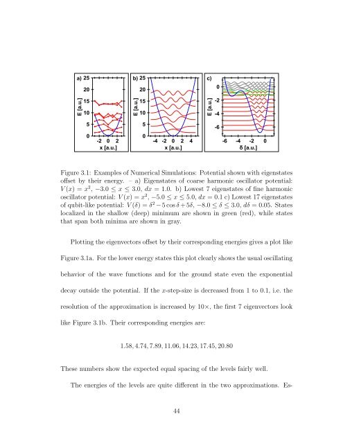
- Page 78 and 79: Figure 3.2: Simulation of LC Oscill
- Page 80 and 81: Table 3.1: Transition Matrix Elemen
- Page 82 and 83: with ω mn = Em−En . Multiplying
- Page 84 and 85: α, it can be ignored. Thus, the in
- Page 86 and 87: e solved exactly: A(t + ∆t) = e
- Page 88 and 89: qubits would be simulated using: A(
- Page 90 and 91: This calculation assumes that the s
- Page 92 and 93: Decoherence consists of two parts:
- Page 94 and 95: Note the difference in signs of the
- Page 97 and 98: Chapter 4 Designing the Phase Qubit
- Page 99 and 100: mutual inductance between the qubit
- Page 101 and 102: During the measurement, the | 1 〉
- Page 103 and 104: the right impedance transformation
- Page 105 and 106: excitations. Since these are a pote
- Page 107 and 108: Figure 4.3: Squid I/V Traces - a) L
- Page 109 and 110: Figure 4.5: Qubit Integrated Circui
- Page 111 and 112: The geometry of the qubit junction
- Page 113 and 114: squid loop. Thus, this tool can be
- Page 115: now, amorphous silicon seems to pro
- Page 118 and 119: Figure 5.1: L-Edit Mask Layout Tool
- Page 120 and 121: Figure 5.2: Fabrication Building Bl
- Page 122 and 123:
Figure 5.3: Photolithography and Et
- Page 124 and 125:
times the removal can be a bit tric
- Page 126 and 127:
Figure 5.4: Clearing Vias from Nati
- Page 128 and 129:
5.6 Junction Layers 5.6.1 Oxidation
- Page 130 and 131:
top wiring layer to protect all low
- Page 132 and 133:
104
- Page 134 and 135:
6.1 Physical Quality Control during
- Page 136 and 137:
6.1.3 Atomic Force Microscopy To re
- Page 138 and 139:
Figure 6.1: 4-Wire Measurement - a)
- Page 140 and 141:
6.3 Quantum Measurements at 25 mK 6
- Page 142 and 143:
seems to be a box machined out of s
- Page 144 and 145:
Figure 6.2: Dilution Refrigerator W
- Page 146 and 147:
cessing data. This protects the vol
- Page 148 and 149:
6.3.9 Anritsu Microwave Source The
- Page 150 and 151:
122
- Page 152 and 153:
ment, the scalability requirements,
- Page 154 and 155:
people without any formal training
- Page 156 and 157:
7.2.4 Performance Last, but certain
- Page 158 and 159:
or a Client Module. Client Modules
- Page 160 and 161:
second Module talks to all these an
- Page 162 and 163:
puters to talk to each other. Usual
- Page 164 and 165:
7.3.4 Performance Addressing the Pe
- Page 166 and 167:
is designed such that the LabRAD Ma
- Page 168 and 169:
Table 7.3: LabRAD Type Annotations
- Page 170 and 171:
listed in Table 7.3. For transmissi
- Page 172 and 173:
Architecture to manage network conn
- Page 174 and 175:
Manager. In fact, in our lab, the o
- Page 176 and 177:
waiting for their completion. The C
- Page 178 and 179:
mentation of pipelining and certain
- Page 180 and 181:
Since the API guarantees that all R
- Page 182 and 183:
one microwave line for X/Y-rotation
- Page 184 and 185:
7.5.3 DC Rack Server The DC Rack Se
- Page 186 and 187:
data taking on the lab servers and
- Page 188 and 189:
keys and the ability to set Context
- Page 190 and 191:
a certain time. 7.5.9 Optimizer Cli
- Page 192 and 193:
ters read from different sub-direct
- Page 194 and 195:
efore the execution of the sequence
- Page 196 and 197:
can achieve very-close-to hardware
- Page 198 and 199:
type to provide a one-stop location
- Page 200 and 201:
172
- Page 202 and 203:
8.1 Squid I/V Response As explained
- Page 204 and 205:
a digital signal via the use of a c
- Page 206 and 207:
energy landscape (see Chapter 2.2.3
- Page 208 and 209:
Figure 8.3: Squid Steps Failure Mod
- Page 210 and 211:
At this point, the squid ramp can b
- Page 212 and 213:
starts to tunnel to the neighboring
- Page 214 and 215:
Figure 8.5: General Bias Sequence -
- Page 216 and 217:
Figure 8.7: Spectroscopy - a) Bias
- Page 218 and 219:
Figure 8.8: Rabi Oscillation - a) B
- Page 220 and 221:
ensemble with respect to each other
- Page 222 and 223:
Figure 8.10: T 1 - a) Bias sequence
- Page 224 and 225:
Figure 8.11: Ramsey - a) Bias seque
- Page 226 and 227:
phase shift into the middle of the
- Page 228 and 229:
photon excitation behaves similarly
- Page 230 and 231:
is desirable to modularize the cont
- Page 232 and 233:
sequence was run. This allows for t
- Page 234 and 235:
possible to read out all qubits cor
- Page 236 and 237:
simultaneous application of such me
- Page 238 and 239:
Figure 9.4: Capacitive Coupling Swa
- Page 240 and 241:
Figure 9.6: Capacitive Coupling Pha
- Page 242 and 243:
a phase difference of 0 ◦ rather
- Page 244 and 245:
Figure 9.7: Fine Spectroscopy of Re
- Page 246 and 247:
Figure 9.8: Swapping Photon into Re
- Page 248 and 249:
esonator. The latter calibration is
- Page 250 and 251:
Figure 9.11: Resonator T 1 - a) Seq
- Page 252 and 253:
224
- Page 254 and 255:
He does not throw dice” [Einstein
- Page 256 and 257:
(independent of which axis it is),
- Page 258 and 259:
of E xy is measured by expressing i
- Page 260 and 261:
For a measurement of two particles
- Page 262 and 263:
10.2.1 Photons The first and most n
- Page 264 and 265:
10.2.3 Ion and Photon In the attemp
- Page 266 and 267:
238
- Page 268 and 269:
11.1 State Preparation Since the ab
- Page 270 and 271:
Figure 11.1: Bell State Preparation
- Page 272 and 273:
Table 11.1: Entangled State Density
- Page 274 and 275:
Figure 11.2: Bell Measurements - a)
- Page 276 and 277:
11.2.3 Statistical Analysis For the
- Page 278 and 279:
11.3 Calibration The most difficult
- Page 280 and 281:
Table 11.4: Sequence Parameters - R
- Page 282 and 283:
ally determine an optimal value for
- Page 284 and 285:
ages are based on this method, incl
- Page 286 and 287:
equires to converge. Since the algo
- Page 288 and 289:
Table 11.7: Bell Violation Results
- Page 290 and 291:
Table 11.9: Error Budget - Capaciti
- Page 292 and 293:
Table 11.10: Bell Violation Results
- Page 294 and 295:
Bell inequality. To make this claim
- Page 296 and 297:
Table 11.12: Bell Violation Results
- Page 298 and 299:
11.5.2 Dependence of S on Sequence
- Page 300 and 301:
point where the measurement happens
- Page 302 and 303:
The second qubit is not driven and
- Page 304 and 305:
Figure 11.6: Resonator Coupled Samp
- Page 306 and 307:
From the resulting states, the 16 p
- Page 308 and 309:
Table 11.14: Error Budget - Resonat
- Page 310 and 311:
Table 11.15: Bell Violation Results
- Page 312 and 313:
sponding to a violation by 244.0σ.
- Page 314 and 315:
educe energy decay and dephasing an
- Page 316 and 317:
John F. Clauser, Michael A. Horne,
- Page 318 and 319:
J. Majer, J. M. Chow, J. M. Gambett
- Page 320:
Matthias Steffen, M. Ansmann, Rados