PDF (double-sided) - Physics Department, UCSB - University of ...
PDF (double-sided) - Physics Department, UCSB - University of ... PDF (double-sided) - Physics Department, UCSB - University of ...
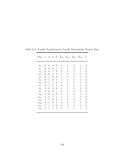
(independent of which axis it is), they will yield an opposite outcome with certainty. But since measurements along orthogonal axes do not commute, quantum mechanics not only forbids a simultaneous prediction of the outcome of all possible measurements, but states that this information is not present in the state of the two particles before the measurement. Instead, a measurement of particle A instantaneously collapses the wave-function (changes the state) of particle B despite the fact that they are causally disconnected by their distance. Einstein called this non-local effect of entanglement the “spooky action at a distance”. A possible local hidden variable theory would instead state that the particles agree on all possible measurement outcomes before their separation. This agreement would be contained in the state of the particles in extra unmeasured degrees of freedom, the hidden variables. If the measurements of particles A and B are limited to two possible choices of axes each, a and a ′ as well as b and b ′ , and the outcomes are encoded in binary (1 or 0), this agreement implies that the particles have to choose at the time of separation to belong to one of the 16 possible populations shown in Table 10.1. Next, one defines a correlation measurement E xy which takes the value 1 if the outcome of a measurement of particle A along axis x and particle B along axis y yields the same result for both particles and a value of −1 for opposite results. For experimental implementation, the expectation value 228
Table 10.1: Possible Populations for Locally Deterministic Particle Pairs Pop. a a ′ b b ′ E ab E a ′ b E ab ′ E a ′ b ′ S n 0 0 0 0 0 1 1 1 1 2 n 1 0 0 0 1 1 1 -1 -1 2 n 2 0 0 1 0 -1 -1 1 1 -2 n 3 0 0 1 1 -1 -1 -1 -1 -2 n 4 0 1 0 0 1 -1 1 -1 -2 n 5 0 1 0 1 1 -1 -1 1 2 n 6 0 1 1 0 -1 1 1 -1 -2 n 7 0 1 1 1 -1 1 -1 1 2 n 8 1 0 0 0 -1 1 -1 1 2 n 9 1 0 0 1 -1 1 1 -1 -2 n 10 1 0 1 0 1 -1 -1 1 2 n 11 1 0 1 1 1 -1 1 -1 -2 n 12 1 1 0 0 -1 -1 -1 -1 -2 n 13 1 1 0 1 -1 -1 1 1 -2 n 14 1 1 1 0 1 1 -1 -1 2 n 15 1 1 1 1 1 1 1 1 2 229
- Page 206 and 207: energy landscape (see Chapter 2.2.3
- Page 208 and 209: Figure 8.3: Squid Steps Failure Mod
- Page 210 and 211: At this point, the squid ramp can b
- Page 212 and 213: starts to tunnel to the neighboring
- Page 214 and 215: Figure 8.5: General Bias Sequence -
- Page 216 and 217: Figure 8.7: Spectroscopy - a) Bias
- Page 218 and 219: Figure 8.8: Rabi Oscillation - a) B
- Page 220 and 221: ensemble with respect to each other
- Page 222 and 223: Figure 8.10: T 1 - a) Bias sequence
- Page 224 and 225: Figure 8.11: Ramsey - a) Bias seque
- Page 226 and 227: phase shift into the middle of the
- Page 228 and 229: photon excitation behaves similarly
- Page 230 and 231: is desirable to modularize the cont
- Page 232 and 233: sequence was run. This allows for t
- Page 234 and 235: possible to read out all qubits cor
- Page 236 and 237: simultaneous application of such me
- Page 238 and 239: Figure 9.4: Capacitive Coupling Swa
- Page 240 and 241: Figure 9.6: Capacitive Coupling Pha
- Page 242 and 243: a phase difference of 0 ◦ rather
- Page 244 and 245: Figure 9.7: Fine Spectroscopy of Re
- Page 246 and 247: Figure 9.8: Swapping Photon into Re
- Page 248 and 249: esonator. The latter calibration is
- Page 250 and 251: Figure 9.11: Resonator T 1 - a) Seq
- Page 252 and 253: 224
- Page 254 and 255: He does not throw dice” [Einstein
- Page 258 and 259: of E xy is measured by expressing i
- Page 260 and 261: For a measurement of two particles
- Page 262 and 263: 10.2.1 Photons The first and most n
- Page 264 and 265: 10.2.3 Ion and Photon In the attemp
- Page 266 and 267: 238
- Page 268 and 269: 11.1 State Preparation Since the ab
- Page 270 and 271: Figure 11.1: Bell State Preparation
- Page 272 and 273: Table 11.1: Entangled State Density
- Page 274 and 275: Figure 11.2: Bell Measurements - a)
- Page 276 and 277: 11.2.3 Statistical Analysis For the
- Page 278 and 279: 11.3 Calibration The most difficult
- Page 280 and 281: Table 11.4: Sequence Parameters - R
- Page 282 and 283: ally determine an optimal value for
- Page 284 and 285: ages are based on this method, incl
- Page 286 and 287: equires to converge. Since the algo
- Page 288 and 289: Table 11.7: Bell Violation Results
- Page 290 and 291: Table 11.9: Error Budget - Capaciti
- Page 292 and 293: Table 11.10: Bell Violation Results
- Page 294 and 295: Bell inequality. To make this claim
- Page 296 and 297: Table 11.12: Bell Violation Results
- Page 298 and 299: 11.5.2 Dependence of S on Sequence
- Page 300 and 301: point where the measurement happens
- Page 302 and 303: The second qubit is not driven and
- Page 304 and 305: Figure 11.6: Resonator Coupled Samp
Table 10.1: Possible Populations for Locally Deterministic Particle Pairs<br />
Pop. a a ′ b b ′ E ab E a ′ b E ab ′ E a ′ b ′ S<br />
n 0 0 0 0 0 1 1 1 1 2<br />
n 1 0 0 0 1 1 1 -1 -1 2<br />
n 2 0 0 1 0 -1 -1 1 1 -2<br />
n 3 0 0 1 1 -1 -1 -1 -1 -2<br />
n 4 0 1 0 0 1 -1 1 -1 -2<br />
n 5 0 1 0 1 1 -1 -1 1 2<br />
n 6 0 1 1 0 -1 1 1 -1 -2<br />
n 7 0 1 1 1 -1 1 -1 1 2<br />
n 8 1 0 0 0 -1 1 -1 1 2<br />
n 9 1 0 0 1 -1 1 1 -1 -2<br />
n 10 1 0 1 0 1 -1 -1 1 2<br />
n 11 1 0 1 1 1 -1 1 -1 -2<br />
n 12 1 1 0 0 -1 -1 -1 -1 -2<br />
n 13 1 1 0 1 -1 -1 1 1 -2<br />
n 14 1 1 1 0 1 1 -1 -1 2<br />
n 15 1 1 1 1 1 1 1 1 2<br />
229


