PDF (double-sided) - Physics Department, UCSB - University of ...

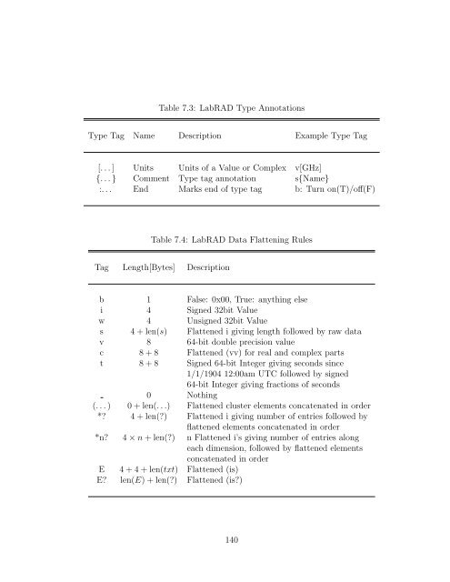
Table 7.3: LabRAD Type Annotations
Type Tag Name Description Example Type Tag
[. . . ] Units Units of a Value or Complex v[GHz]
{. . . } Comment Type tag annotation s{Name}
:. . . End Marks end of type tag b: Turn on(T)/off(F)
Table 7.4: LabRAD Data Flattening Rules
Tag Length[Bytes] Description
b 1 False: 0x00, True: anything else
i 4 Signed 32bit Value
w 4 Unsigned 32bit Value
s 4 + len(s) Flattened i giving length followed by raw data
v 8 64-bit double precision value
c 8 + 8 Flattened (vv) for real and complex parts
t 8 + 8 Signed 64-bit Integer giving seconds since
1/1/1904 12:00am UTC followed by signed
64-bit Integer giving fractions of seconds
0 Nothing
(. . . ) 0 + len(. . .) Flattened cluster elements concatenated in order
*? 4 + len(?) Flattened i giving number of entries followed by
flattened elements concatenated in order
*n? 4 × n + len(?) n Flattened i’s giving number of entries along
each dimension, followed by flattened elements
concatenated in order
E 4 + 4 + len(txt) Flattened (is)
E? len(E) + len(?) Flattened (is?)
140