Homework 6 - Solutions - Physics Department, UCSB
Homework 6 - Solutions - Physics Department, UCSB
Homework 6 - Solutions - Physics Department, UCSB

You also want an ePaper? Increase the reach of your titles
YUMPU automatically turns print PDFs into web optimized ePapers that Google loves.
<strong>Homework</strong> 6 - <strong>Solutions</strong><br />
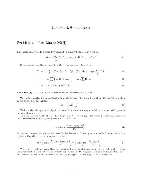
Problem 1 - Non-Linear M(H)<br />
The Hamiltonian of a Heisenberg ferrromagnet in a magnetic field H is given by<br />
H = −J ∑ ∑<br />
S i · S J − gµ B H · S i , J > 0 (1)<br />
〈ij〉<br />
i<br />
It was seen in class that in mean field theory we can study the system<br />
H = −J ∑ [<br />
]<br />
∑<br />
〈S i 〉 · S j + S i · 〈S j 〉 − 〈S i 〉 · 〈S j 〉 − gµ B H · S i (2)<br />
〈ij〉<br />
i<br />
= −zJ ∑ (<br />
)<br />
∑<br />
m · S i + const. − gµ B H · S i (3)<br />
i<br />
i<br />
= − ∑ i<br />
(zJm + gµ B H) · S i (4)<br />
where m = 〈S i 〉 and z equals the number of nearest neighbour lattice sites.<br />
We saw in class that the magnetization for a spin-1/2 particle interacting with an effective field h is given<br />
by the solution to the equation<br />
m = 1 [ ] h<br />
2 tanh (5)<br />
2kT<br />
We know that the spins will align in the same direction as the magnetic field so that m and H point in<br />
the same direction.<br />
Then, in our system, the effective field is given by h = zJm + ζgµ B |H|, where ζ = sign(H). Therefore,<br />
the magnetization is given by the solution to the equation<br />
m = 1 [ ]<br />
zJm +<br />
2 tanh ζgµB |H|<br />
2kT<br />
(6)<br />
We also saw in class that the critical point for the Heisinberg ferromagnet in mean field theory is at kT c =<br />
zJ/4. Subbing this in for our temperature gives<br />
m = 1 [ ] 2(zJm +<br />
2 tanh ζgµB |H|)<br />
= 1 [<br />
zJ<br />
2 tanh 2m + 2ζgµ ]<br />
B|H|<br />
(7)<br />
zJ<br />
When H is small, we know that the magnetization m is also small near the critical point T c , since<br />
the magnetization is zero above the critical temperature and the magnetization is a continuous function of<br />
temperature for this model. Therefore we can Taylor expand our tanh(x) ≈ x − x 3 /3 function<br />
1
m = 1 [<br />
2m + 2ζgµ B|H|<br />
+ 1 (<br />
2m + 2ζgµ ) 3 ]<br />
B|H|<br />
(8)<br />
2 zJ 3<br />
zJ<br />
0 = ζgµ B|H|<br />
+ 1 (<br />
2m + 2ζgµ ) 3<br />
B|H|<br />
(9)<br />
zJ 6<br />
zJ<br />
( ) 1/3 6ζgµB |H|<br />
⇒ 2m ≈<br />
+ O(H) (10)<br />
zJ<br />
( ) 1/3 6gµB<br />
|H| 1/3 (11)<br />
m = sign(H) 1 2<br />
zJ<br />
Where above I expanded the equation above to lowest nonvanishing order in both m and H.<br />
Therefore<br />
M = gµ B m = sign(H) gµ ( ) 1/3<br />
B 6gµB<br />
|H| 1/3 (12)<br />
2 zJ<br />
2
Problem 2 - Quantum transverse-field Ising model<br />
Part (a)<br />
We start with the spin 1/2 Hamiltonian, and apply the mean field approximation:<br />
H = −J ∑ ∑<br />
Si z Sj<br />
z − h ⊥ Si x (13)<br />
〈ij〉<br />
i<br />
≈ −J ∑ ∑<br />
Si z 〈Sj z 〉 + 〈Si z 〉Sj z − 〈Si z 〉〈Sj z 〉 − h ⊥ Si x (14)<br />
〈ij〉<br />
i<br />
= ∑ (−zJm)Si z − h ⊥ Si x + const (15)<br />
i<br />
= − ∑ i<br />
h · S with h = (h ⊥ , 0, zJm) (16)<br />
where m = 〈Si z 〉. Therefore, our mean field Hamiltonian can be written as a set of spins in an effect field<br />
h eff = (h ⊥ , 0, zJm)<br />
Part (b)<br />
Now, we assume that we are at zero temperature and that each spin is aligned fully with the effect field<br />
h eff .<br />
Therefore, we now that S points in the direction (h ⊥ , 0, Jzm). We also know that |S| = S = 1/2. Then,<br />
we can write<br />
S i = 1 Jzmẑ + h<br />
√ ⊥ˆx<br />
(17)<br />
2 J 2<br />
z 2 m 2 + h 2 ⊥<br />
Since this is the proper normalized spin-1/2 vector which points in the h eff direction.<br />
Since all spins point in the same direction, the magnetization is just the z component of this spin vector<br />
m = 〈Si z 〉 = 1 Jzm<br />
√ (18)<br />
2 J 2<br />
z 2 m 2 + h 2 ⊥<br />
⇒ m 2 J 2 z 2 m 2<br />
=<br />
4(J 2 z 2 m 2 + h 2 ⊥ ) (19)<br />
0 = 4J 2 z 2 m 4 + (4h 2 ⊥ − J 2 z 2 )m 2 (20)<br />
Part (c)<br />
Therefore, for a given transverse field h ⊥ , the magnetization is given by the solution to the equation<br />
Solving this gives<br />
We see that for<br />
occurs when<br />
Therefore<br />
h 2 ⊥<br />
J 2 z 2<br />
4J 2 z 2 m 4 + 42h 2 ⊥ − J 2 z 2 )m 2 = 0 (21)<br />
m 2 (4J 2 z 2 m 2 + (4h 2 ⊥ − J 2 z 2 )) = 0 (22)<br />
⇒ m = 0 or m = ±√<br />
1<br />
4 − h2 ⊥<br />
J 2 z 2 (23)<br />
> 1 4 , the only solution to this equation is at m = 0. Therefore the critical field h c<br />
h2 ⊥<br />
J 2 z<br />
= 1 2 4 (i.e when h ⊥ = Jz/2). When h ⊥ > h c , we have that m(h ⊥ ) = 0<br />
1<br />
m(h ⊥ ) = ±√<br />
4 − h2 ⊥<br />
J 2 z 2 , for h ⊥ < h c where h c = Jz<br />
2<br />
(24)<br />
3
Problem 3 - Low Temperature Magnetization of the Heisenberg Ferromagn<br />
∫ ∞<br />
〈STOT〉/N z = +S − n B (ε)dε (25)<br />
ε=0<br />
(26)<br />
The number of magnons at a given temperature T is given by<br />
∑<br />
∫<br />
n k = dεD(ε)〈n(ε)〉 (27)<br />
k<br />
The factor of D(ε) is the number of frequency modes k which exist at a given energy ω. For a given<br />
wavevector k, we have the number of states within a sphere of radius k is N(k) = (2π) −3 ( 4 3 πk3 ). Then the<br />
number of states within a shell of thickness dε is:<br />
Therefore<br />
D(ε)dε = dN(k) dk<br />
dk dε dε = 1 dk<br />
4πk2 dε (28)<br />
(2π)<br />
3<br />
dε<br />
(29)<br />
〈S z TOT〉/N = S − 4π<br />
(2π) 3 ∫ kF<br />
k=0<br />
k 2<br />
dk (30)<br />
e βck2 − 1<br />
≈ S − 1 ∫ ∞<br />
k 2<br />
2π 2 dk<br />
0 e βck2 − 1<br />
(31)<br />
(32)<br />
where we make the approximation that the upper bound on the integral goes to infinity since n B (k) → 0<br />
exponentially fast as k becomes large.<br />
Now, let x = βck 2 So that dx = 2βck dk and we can write the integral above as<br />
〈S z TOT〉/N = S − 1<br />
2π 2 ∫ ∞<br />
0<br />
dx x 1<br />
√<br />
2βc βc e x − 1<br />
(33)<br />
= S − 1 ∫ ∞<br />
4π 2 c (kT x<br />
)3/2<br />
e x dx (34)<br />
− 1<br />
= S − 1 (kT ) 3/2<br />
12 c<br />
where in the last line I used the fact that the integral over x is equal to π 2 /6<br />
0<br />
(35)<br />
4