Mossbauer Spectroscopy of 57Fe - MIT

Mossbauer Spectroscopy of 57 F e
Dennis V. Perepelitsa ∗
MIT Department of Physics
(Dated: April 6, 2007)
Using recoilless Mossbauer spectroscopy methods, we investigate the atomic absorption spectra of
the 14.4keV transition in 57 F e compounds. The natural linewidth of this transition is determined
to the correct order of magnitude with χ 2 ν = .75. Hyperfine energy shifts in iron oxide and iron
sulfate are investigated and measured. The ratio of ground and excited state magnetic moment in
57 F e is found to be −1.73(2). The internal magnetic field in metallic iron is found to be 350(2) kG.
The phenomenon of relativistic time dilation is confirmed with χ 2 ν = 1.52.
1. INTRODUCTION
In 1958, Rudolf Mossbauer devised a method that allowed
the phenomenon of practical resonance absorption
to occur. Using this method, absorption spectroscopy
become possible at a much higher resolution than was
otherwise available at the time. Within the next several
years, scientists investigated the details of several atomic
spectra, measuring hyperfine splitting effects and other
values with heretofore unrealizable accuracy.
In this experiment, we probe the absorption spectra of
the 14.4 keV line of species containing 57 F e.
2. THEORY
Mossbauer [1] presents how to achieve the phenomenon
of resonance absorption by fixing the emission source in
a crystal lattice and moving it gently with respect to the
absorption source. The first order approximation of the
new energy E ′ given velocity v is given by the Doppler
effect:
(
E ′ = E 0 1 + v )
c
(1)
The natural linewidth of an absorption line reflects a
fundamental quantum property of incoming radiation -
the uncertainty in the energy is tied to the uncertainty in
the lifetime of the excited state through Heisenberg’s relation:
∆E∆τ = /2. The spectral line has a Lorentzian
profile centered on E 0 with intensity I 0 and full-width
half-maximum (FWHM) Γ:
) 2
(
I Γ 0 2
L(E) =
(E − E 0 ) 2 + ( )
Γ 2
(2)
2
Of course, both the emission and absorption line have
the above profile, with intensities I 0 and σ 0 , respectively.
To model the observed absorption spectrum after it has
∗ Electronic address: dvp@mit.edu
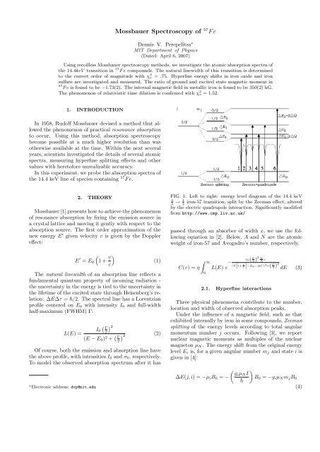
FIG. 1: Left to right: energy level diagram of the 14.4 keV
3
→ 1 iron-57 transition, split by the Zeeman effect, altered
3 2
by the electric quadrupole interaction. Significantly modified
from http://www.cmp.liv.ac.uk/
passed through an absorber of width x, we use the following
equation in [2]. Below, A and N are the atomic
weight of iron-57 and Avogadro’s number, respectively.
C(v) = η
∫ ∞
0
L(E) e
−
σ 0( Γ 2 ) 2 N
A
x
(E[1+ v c ]−E 0 −∆C) 2 +( Γ 2 ) 2 dE (3)
2.1. Hyperfine interactions
Three physical phenomena contribute to the number,
location and width of observed absorption peaks.
Under the influence of a magnetic field, such as that
exhibited internally by iron in some compounds, Zeeman
splitting of the energy levels according to total angular
momentum number j occurs. Following [3], we report
nuclear magnetic moments as multiples of the nuclear
magneton µ N . The energy shift from the original energy
level E i is, for a given angular number m j and state i is
given in [4]:
( )
gi µ N I
∆E(j, i) = −µ i B 0 = − B 0 = −g i µ N m j B 0
(4)

2
Where µ i is the magnetic moment, expressed as a fraction
g i of the nuclear magneton µ N = 3.15 × 10 −12
eV/gauss, and B 0 is the magnetic field of the nucleus.
Since m j comes in multiples of one-half, the observed
spacing between two energy levels with different m j numbers
will some integer multiple of g i µ N B 0 .
The quadrupole interaction is caused by an electric
quadrupole moment in the atomic crystal lattice. The
ground state of the atom is not affected, but the first
excited state is split into sublevels that correspond to
different magnitudes of m j . Let q be the gradient of the
electric potential and e 2 Q the quadrupole moment. The
energy shift ∆Q for the m j = ± 3 2 sublevels (the m j = ± 1 2
energy shift has the same magnitude but opposite sign)
is given in [5]:
∆Q =
qe2 Q [
3m
2
4j(2j − 1) j − j(j + 1) ] = 1 4 qe2 Q (5)
An energy diagram of combined Zeeman splitting and
quadrupole-interaction is given in Figure 1.
The chemical isomer shift is caused by a difference in
chemical environment between source and absorber. It
has the effect of shifting all energies by a small amount.
A more detailed description is given in [5].
2.2. Relativistic effects
The 57 F e atoms in the lattice oscillate at higher frequencies
in at higher temperatures, leading to an energy
shift of the accompanying absorption peak from
the Doppler effect. The first-order Doppler effect, which
replicates the classical one, negates itself in the aggregate.
Theoretically, however, the second-order term contributes
to a general energy shift. From [6], in the classical
limit, the temperature dependence of this shift ∆E T
is
d ∆E T
dT E = − 3k
2Mc 2 (6)
3. EXPERIMENTAL SETUP
The heart of our setup is the ASA-S700A Mossbauer
Drive Module which drives a 57 Co source connected to
the end of a piston.
57 Co decays by beta capture to
57 F e in an excited state, which emit 14.4keV gamma rays
through atomic de-excitation directed at a proportional
counter. The piston is moved periodically as a sawtooth
function of time by the drive circuit, and the desired
absorption source is placed between it and the counter.
The counter is connected in series to a high-voltage discriminator
and signal amplifier, which directs DC voltage
pulses to a central multi-channel scaler (MSC) that vary
linearly with the observed amount of counts.
FIG. 2: Piston-mounted decay source and associated absorption
spectrum measurement chain with adjacent laser interferometry
setup for velocity calculation.
The MSC setup directs the Mossbauer Drive Module
and receives the amplified voltage pulses, which is sends
to a personal computer for display and analysis. The
piston is driven at a frequency of 6Hz and integrated
count times over 1024 sweeps of T ≈ 200µs. To analyze
signal stability, the velocity and drive of the MDM was
displayed on a digital oscilloscope, and triggered by the
rising edge of the MSC.
An adjacent interferometer setup with a laser of wavelength
λ = 632.8 nm detailed in Figure 2 determines the
velocity of the piston at any given time. Consider the i th
channel of the MCS. In the integration time T , the path
taken by the beam reflecting off the piston travels a distance
2T V i . At each full wavelength of interference, the
photodiode records a count. If the cycle is repeated N
times and C i total counts recorded, the velocity of that
channel is V i = Ciλ
2NT
. The output of the photodiode is
amplified and replaces the input from the proportional
counter during calibration runs.
3.1. Methodology
Before an energy spectrum reading, we attempted to
take a velocity calibration using the interferometer setup
described above. Due to equipment problems on some
days, we calibrated the energy spectrum using the two
outer or inner peaks of the metallic iron absorption spectrum.
The Drive Module maximum piston velocity was set
to 80mm/s for most spectra, and 10mm/s when taking
the sulfate and temperature-dependent data. The
fidelity knob was manually adjusted each time to yield a
crisp velocity curve. After activating the piston motor,
we waited a sufficient time to allow the velocity signal
to stabilize before performing a reading. In all cases,

3
TABLE I: Measured atomic transition energies in enriched
metallic iron and iron oxide.
Transition
57 F e F e 2O 3
3/2 → 1/2 −2.79 ± .01 × 10 −7 eV −4.17 ± .01 × 10 −7 eV
1/2 → 1/2 −1.62 ± .01 × 10 −7 eV −2.20 ± .01 × 10 −7 eV
−1/2 → 1/2 −0.41 ± .01 × 10 −7 eV −.41 ± .01 × 10 −7 eV
1/2 → −1/2 0.40 ± .01 × 10 −7 eV .86 ± .01 × 10 −7 eV
−1/2 → −1/2 1.57 ± .01 × 10 −7 eV 2.61 ± .01 × 10 −7 eV
−3/2 → −1/2 2.68 ± .01 × 10 −7 eV 4.30 ± .01 × 10 −7 eV
FIG. 3: Plot of fractional energy shift against temperature.
we recorded absorption spectra until the low absorption
peaks and background noise differed by several hundred
counts.
To determine the natural line width of enriched iron-
57, we recorded the absorption spectra of sodium ferrocyanide
(Na 3 F e(CN) 6 ) for widths of 0.1, 0.25 and 0.5
mg/cm 2 . Hyperfine interactions were observed in the absorption
spectra of metallic iron (enriched 57 F e), iron oxide
(F e 2 O 3 ) and iron sulfates (F e 2 (SO 4 ) 3 and F e(SO 4 )).
Finally, we placed a metallic iron sample in a resistance
heater and recorded its absorption spectra at four values
of the temperature.
∆E 1 . The results are
∆E 0 = (1.99 ± .01) × 10 −7 eV
∆E 1 = −(1.15 ± .01) × 10 −7 eV (7)
From these facts, (4) and the established value of µ 0
in [3], we can calculate ratio of the ground state and first
excited state magnetic moment and the internal magnetic
field. Our results are summarized in Table II.
4.3. Hyperfine interactions in F e 2O 3
4. DATA ANALYSIS
4.1. Natural linewidth of 57 F e
We make two fundamental simplifying assumptions
when manipulating (3). We estimate that it can be approximated
with a Lorentzian profile, and that the measured
full-width of the peak will, when extrapolated linearly,
give the natural linewidth. Plotting the full-width
half-maximum against absorber thickness and computing
the χ 2 ν = .75 least-squares linear fit, we obtain the
linewidth intercept at zero thickness to be (1.2±.1)×10 −8
eV.
4.2. Zeeman splitting in enriched 57 F e
A non-linear fit with χ 2 ν = 1.19 to the data using Poisson
uncertainties (with the consequence that the bottom
of the absorption peaks were more heavily weighted) using
six Lorentzian profiles and a background distribution
was obtained. The data is displayed in Table I. As expected,
the average of the two central peaks coincides
with the zero velocity value to within the derived uncertainty.
To find the ground state energy split ∆E 0 , we take the
weighted average [7] of the differences between transitions
from different ground state sublevels to the same excited
state sublevels. We use a similar method to determine
A similar fitting process resulted in the data in Table
I. As indicated in Figure 1, we must account for an
additional quadrupole shift ∆Q in the excited substates.
Using linear combinations of the transition energies, we
can derive the following values:
∆E 0 = (3.04 ± .01) × 10 −7 eV
∆E 1 = −(1.78 ± .01) × 10 −7 eV
∆Q = −(7.0 ± .2) × 10 −9 eV (8)
There are several interesting features here. The energy
shifts are larger than those in metallic iron by a
factor of (1.53 ± .02), and correspond to an increased internal
magnetic field. The ratio of ground and excited
state magnetic moments remains the same, within error.
The quadrupole shift is in the opposite direction as illustrated
in Figure 1, and this leads to a negative value for
the product of the field gradient and quadrupole moment
qe 2 Q = −(2.8 ± .01) × 10 −8 eV . Finally, we calculate the
(off-center energy) chemical shift ∆C between metallic
iron and F e 2 O 3 . Our results are summarized in Table II.
4.4. Hyperfine interactions in F eSO 4 and F e 2(SO 4) 3
Examination of the spectra revealed that F eSO 4 exhibited
a quadrupole splitting of the first excited state,
while F e 2 SO 4 did not. The quadrupole and chemical
shifts are detailed in Table II.

4
TABLE II: Summary of experimental results. The horizontal
linebreaks correspond to separations between different
species. They are, in order: metallic iron, iron oxide, iron
(II) sulfate and iron (III) sulfate.
Property Derived Value Expected Result Deviation
Γ 1.2(1) × 10 −8 eV 4.7(1) × 10 −9 eV -
∆E T
E
−2.29(22) −2.09(6) ≤ 1σ
×10 −15 eV·K −1 ×10 −15 eV·K −1
µ 0/µ 1 −1.73(2) −1.75(1) ≤ 1σ
B 0 351(2) kG 330(2) kG 6%
d
dT
µ 0/µ 1 −1.71(2) −1.77(2) ≤ 3σ
B 0 534(2) kG 513(2) kG 4%
∆Q 7.0(2) × 10 −9 eV 5.7(1.4) × 10 −9 eV ≤ 1σ
∆C 2.8(1) × 10 −8 eV 2.25(14) × 10 −8 eV ≤ 4σ
∆Q 6.2(1) × 10 −8 eV 6.7(2) × 10 −8 eV ≤ 3σ
∆C 1.60(7) × 10 −7 eV 1.54(2) × 10 −7 ≤ 1σ
∆C 2.2(1) × 10 −8 eV 2.6(2) × 10 −8 eV ≤ 2σ
4.5. Temperature Coefficient of 57 F e
Plotting the off-center energy shift against temperature
and computing the χ 2 ν = 1.53 least-squares linear
d
fit, we obtain the temperature dependence
dE
−(2.29±.22)×10 −15 eV·K −1 . This is shown in Figure 3.
5. ERROR ANALYSIS
∆E T
E
=
After calibrating the energy spectrum from the velocity
curve, the discrete channel uncertainty due to binning
was 1.2×10 −9 eV. Due to this, we truncate the granularity
of all final results to a resolution of 10 −9 eV. Since the
emission and absorption of gamma radiation are nuclear
events, we model the channel count uncertainty using
Poisson statistics. The error in the independent variable
(energy) is thus much smaller than that in the dependent
variable (counts), and we do not incorporate it. In our
analysis, we do not attempt to model uncertainty in the
recorded temperature.
We fit every absorption spectrum after this calibration
using a standard non-linear gradient descent method.
Our reduced-chi-squared values ranged from 1.0 to 1.5
and indicated appropriate fits and correctly modeled error.
The principal source of error was thus fitted parameter
uncertainty, added in quadrature with the energy
uncertainty. In the case of most measured energy values,
this was on the order of 1%, and higher for derived
values.
When forced to perform an energy calibration using
other energy spectra as a reference, we fit to find the
positions of the reference peak, and assign them energy
values we derived earlier. The calibration energy error
is then added in quadrature to the parameter found by
fitting.
6. CONCLUSIONS
Table II gives a summary of our results. The expected
values are drawn from [5], [8] and [3].
There are several complicating factors in our attempt
to measure the width of the 14.4 keV line. Doppler
smearing of the absorption line from the thermal excitation
of the source, and the imperfect resolution of the
proportional counter both contribute to the widening of
the line. We will have to be satisfied with the fact that
our data is of the correct order of magnitude.
Our experimental results concerning hyperfine interactions
in metallic iron, iron oxide and iron sulfate are in
good agreement with established values, with a caveat.
On a qualitative level, we have confirmed the presence of
absence of several hyperfine interaction phenomena. Iron
(III) exhibits a spherically symmetric charge distribution
around the nucleus, while iron (III) does not. Metallic
iron and iron oxide possess an internal atomic magnetic
field, while ferrocyanide and the sulfates do not.
Quantitatively, many of our measured energy values
seem to be systematically higher by approximately 5%.
This seems to imply a consistent energy miscalibration,
and a topic for further investigation.
The temperature dependence of the energy shift has
been confirmed with χ 2 ν = 1.53. This term cannot be
explained under any classical model, and is a confirmation
that quickly moving particles exhibit time dilation
as predicted by special relativity.
[1] R. Mossbauer, Nobel lecture (1961).
[2] J. L. Staff, Mössbauer spectroscopy, URL http://web.
mit.edu/8.13/www/JLExperiments/JLExp13.pdf.
[3] R. Preston, S. Hanna, and J. Heberle, Phys. Rev. Lett.
128 (1962).
[4] D. J. Griffiths, Introduction to Quantum Mechanics (Pearson
Prentice Hall, 2005), 2nd ed.
[5] O. Kistner and A. Sunyar, Phys. Rev. Lett. 4 (1960).
[6] H. Frauenfelder, The Moessbauer Effect: A Review with a
Collection of Reprints (W.A. Benjamin, Inc., 1962).
[7] P. Bevington and D. Robinson, Data Reduction and Error
Analysis for the Physical Sciences (McGraw-Hill, 2003).
[8] S. DeBenedetti, G. Lang, and R. Ingalis, Physical Review
Letters 6, 60 (1961).
Acknowledgments
DVP gratefully acknowledges Brian Pepper’s equal
partnership, as well as the guidance and advice of
Thomas Walker, Daniel Nezich and Scott Sewell.