Binary Stereo Matching

More documents

Recommendations

Info

lumination may have large variations. Another point we want to mention is that the core algorithm of BSM is based on binary and integer computations, so it will still be fast on embedded or mobile devices which do not have powerful floating point units. The rest of this paper is organized as follows. We review some state-of-the-art local methods in Section 2. Then our cost computation and aggregation approach together with BSM are explained in Section 3. Experimental results and analysis are given in Section 4. Finally we draw conclusion in Section 5 2. State-of-the-Art In this section, we briefly review state-of-the-art local methods. Bleyer et al. estimate a 3D plane at each pixel by applying PatchMatch [1] into stereo matching and their method is currently top-performer among local methods. Hosni et al. [7] aggregate matching cost by computing geodesic distance from all pixels to the window’s center. De-Maeztu et al. [3] and Rhemann et al. [9] both adopt guided filter [5] for cost aggregation and have speed advantages comparing to traditional local methods like [14]. Detailed review of other traditional local methods is proposed in [4, 6, 13]. Overall, most of state-of-the-art local methods use absolute pixel intensity difference for composing cost volume so that their performances drop dramatically under radiometric differences. Some methods explicitly handle radiometric differences like rank and census transform [15], however, their performances on normal images are not so good compared with state-of-the-art local methods [6]. Our binary stereo matching algorithm not only achieves comparable performance with state-of-the-art methods but is also robust to the radiometric differences (especially to exposure changes). 3. Proposed Approach In this section we will explain our approach in detail. Our binary stereo matching algorithm also follows the classical four steps as stated before. In cost computation, our approach is completely different with traditional local methods. We directly introduce BRIEF descriptor [2] into cost computation. Thus, BRIEF descriptor B(x) is calculated for every pixel x in the input image pair. According to [2], B(x) is defined as: B(x) = ∑ 2 i−1 τ(p i , q i ) (2) 1≤i≤n where ⟨p 1 , q 1 ⟩, ⟨p 2 , q 2 ⟩, . . . , ⟨p n , q n ⟩ are n pairs of pixels. Each pair ⟨p i , q i ⟩ is sampled by an isotropic Gaussian distribution in a S × S window, which is centered on pixel x. And τ(p i , q i ) is a binary function which is defined as: τ(p i , q i ) = { 1 : I(pi ) > I(q i ) 0 : I(p i ) ≤ I(q i ) (3) where I(x) denotes the intensity of pixel x. After calculating the descriptor, i.e. a binary string for each pixel, the cost volume is constructed as: C(x, d) = ∥ B(x) XOR B(x d ) ∥ 1 (4) where x d is the corresponding pixel of x with disparity d in another view, XOR is a bitwise xor-operation. In short, C(x, d) measures the hamming distance between two binary strings. 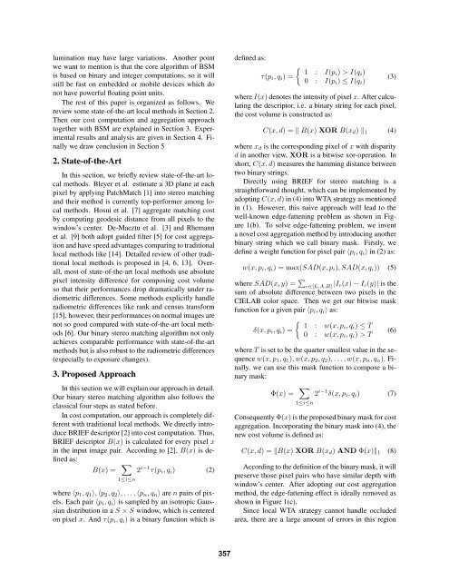Directly using BRIEF for stereo matching is a straightforward thought, which can be implemented by adopting C(x, d) in (4) into WTA strategy as mentioned in (1). However, this naive approach will lead to the well-known edge-fattening problem as shown in Figure 1(b). To solve edge-fattening problem, we invent a novel cost aggregation method by introducing another binary string which we call binary mask. Firstly, we define a weight function for pixel pair ⟨p i , q i ⟩ in (2) as: w(x, p i , q i ) = max(SAD(x, p i ), SAD(x, q i )) (5) where SAD(x, y) = ∑ c∈[L,A,B] |I c(x) − I c (y)| is the sum of absolute difference between two pixels in the CIELAB color space. Then we get our bitwise mask function for a given pair ⟨p i , q i ⟩ as: { 1 : w(x, pi , q δ(x, p i , q i ) = i ) ≤ T (6) 0 : w(x, p i , q i ) > T where T is set to be the quarter smallest value in the sequence w(x, p 1 , q 1 ), w(x, p 2 , q 2 ), . . . , w(x, p n , q n ). Finally, we can use this mask function to compose a binary mask: Φ(x) = ∑ 2 i−1 δ(x, p i , q i ) (7) 1≤i≤n Consequently Φ(x) is the proposed binary mask for cost aggregation. Incorporating the binary mask into (4), the new cost volume is defined as: C(x, d) = ∥B(x) XOR B(x d ) AND Φ(x)∥ 1 (8) According to the definition of the binary mask, it will preserve those pixel pairs who have similar depth with window’s center. After adopting our cost aggregation method, the edge-fattening effect is ideally removed as shown in Figure 1(c). Since local WTA strategy cannot handle occluded area, there are a large amount of errors in this region 357
Table 1. Depth results evaluation. Methods Average Error(%) PatchMatch[8] 4.59 BSM 5.42 CostFilter[9] 5.55 P-LinearS[3] 5.68 GeoSup[7] 5.80 (as shown in Figure 1(c)). Besides, a small amount of random errors appear at non-occluded region due to mismatch. Thus, like other local methods, a depth refinement step is needed for removing these errors [11]. In our BSM algorithm, we propose a voting-based depth refinement method. Firstly, a left/right check using twoview depth maps is performed [8] to classify depth results into two categories: valid and invalid. Then we just refine those invalid pixels’ depth using a voting schema. For an invalid pixel x, its refined depth is calculated as: d x = arg max W (x, d) (9) d∈D d where W (x, d) represents accumulated weight voted from valid pixels, which is defined as: W (x, d) = ∑ p c(x, p) e(x, p) exp(−( + )) (10) λ c λ e where p represents a valid pixel with disparity d. And the accumulated weight is calculated according to bilateral filter [12] where c(x, p) and e(x, p) are distances between two pixels in color and Euclidean space respectively. In our implementation, parameters for bilateral filter are set as: λ c = 9, λ e = 16. As shown in Figure 1(d), errors are corrected after refinement. 4. Experimental Results and Analysis In this section, we conduct a set of experiments to demonstrate the effectiveness of the proposed stereo algorithm. 4.1. Comparison with state-of-the-art To compare with state-of-the-art local methods, we test BSM on standard datasets from Middlebury website [10]. In our implementation, we set n = 4096, S = 26, and the standard variance for the isotropic Gaussian distribution to be 4. We use the same parameters for all datasets. Comparison between our algorithm with other Table 2. Speed evaluation. Methods Processor Running Frequency(Hz) Time(s) BSM 2.67 50 P-LinearS[3] 2.13 94 Errors in unoccluded areas [%] 60 50 40 30 20 10 0 1/1 1/2 1/3 2/1 2/2 2/3 3/1 3/2 3/3 3x3 left/right image combinations BSM CostFilter (a) Different exposure Errors in unoccluded areas [%] 60 50 40 30 20 10 0 1/1 1/2 1/3 2/1 2/2 2/3 3/1 3/2 3/3 3x3 left/right image combinations BSM CostFilter (b) Different lighting Figure 2. <strong>Matching</strong> 3×3 left/right image combinations that differ in exposure or lighting conditions. methods is presented in Table 1. We just list average error rate here to save space and detailed comparison can be found from our submission on Middlebury website [10]. In addition, we give a rough comparison of BSM’s computational time with the fastest local methods. Since different methods are implemented under different platforms and there are many programming techniques (parallel computing or not) which affects the speed of the algorithm, we only choose P-LinearS [3] as representative of the fastest local methods for comparison, which has similar hardware configuration and implementation technique with our method (both algorithms are tested with one core and one process). Table 2 shows test result on Teddy dataset, which involves the largest computational cost among all four datasets. Our algorithm is much faster than [3] using a slightly better CPU. 4.2. Resistance to radiometric differences The traditional four datasets from Middlebury are configured under ideal illumination. For real images, there may be some radiometric changes. Thus, Hirschmuller et al. proposed new datasets incorporating exposure and lighting changes and evaluated some stereo methods on these datasets [6]. These new datasets give rectified image pairs under three different exposures and three lighting conditions. We conduct the same experiment as that mentioned in [6] and use the same evaluation methodology. For comparison, we also test CostFilter[9] on these datasets (using the source code provided by the author). As shown in Figure 2, comparing to CostFilter[9], BSM has much better performance under exposure changes. As for lighting changes, both BSM and CostFilter do not show good performance. As stated in [6], it is of great difficult to handle local radiometric changes caused by changing the location of the light sources. 4.3. Influence of descriptor length It is easy to be proved that our algorithm’s computational complexity is O(whnd max ) (w and h are image width and height respectively). Thus running speed of BSM is mainly determined by the descriptor length n. 358
Page 1: 21st International Conference on Pa

Binary Stereo Matching

Create successful ePaper yourself

Delete template?

Save as template?