Human Detection in Video over Large Viewpoint Changes

Human Detection in Video over Large
Viewpoint Changes
Genquan Duan 1 , Haizhou Ai 1 , and Shihong Lao 2
1 Computer Science & Technology Department, Tsinghua University, Beijing, China
ahz@mail.tsinghua.edu.cn
2 Core Technology Center, Omron Corporation, Kyoto, Japan
lao@ari.ncl.omron.co.jp
Abstract. In this paper, we aim to detect human in video over large
viewpoint changes which is very challenging due to the diversity of human
appearance and motion from a wide spread of viewpoint domain
compared with a common frontal viewpoint. We propose 1) a new feature
called Intra-frame and Inter-frame Comparison Feature to combine
both appearance and motion information, 2) an Enhanced Multiple Clusters
Boost algorithm to co-cluster the samples of various viewpoints and
discriminative features automatically and 3) a Multiple Video Sampling
strategy to make the approach robust to human motion and frame rate
changes. Due to the large amount of samples and features, we propose a
two-stage tree structure detector, using only appearance in the 1 st stage
and both appearance and motion in the 2 nd stage. Our approach is evaluated
on some challenging Real-world scenes, PETS2007 dataset, ETHZ
dataset and our own collected videos, which demonstrate the effectiveness
and efficiency of our approach.
1 Introduction
Human detection and tracking are intensively researched in computer vision in
recent years due to their wide spread of potential applications in real-world tasks
such as driver-aided system, visual surveillance system, etc., in which real time
and high accuracy performance is required.
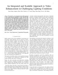
In this paper, our problem is to detect human in video over large viewpoint
changes as shown in Fig. 1. It is very challenging due to the following issues: 1)
A large variation in human appearance over wide viewpoint changes is caused by
different poses, positions and views; 2) Lighting change and background clutter
as well as occlusions make human detection much harder; 3) The diversity of
human motion exists where any direction of movement is possible and the shape
and the size of a human in video may change as he moves; 4) Video frame rates
are often different; 5) The camera is moving sometimes.
The basic idea for human detection in video is to combine both appearance
and motion information. There are mainly three difficult problems to be explored
in this detection task: 1) How to combine both appearance and motion information
to generate discriminative features? 2) How to train a detector to cover such

1248 G. Duan, H. Ai, and S. Lao
Fig. 1: Human detection in video over large viewpoint changes. Samples of three typical
viewpoints and corresponding scenes are given.
a large variation in human appearance and motion over wide viewpoint changes?
3) How to deal with the changes in video frame rate or abrupt motion if using
motion features on several consecutive frames? Viola and Jones [1] first made use
of appearance and motion information in object detection, where they trained
AdaBoosted classifiers with Harr features on two consecutive frames. Later Jones
and Snow [2] extended this work by proposing appearance filter, difference filter
and shifted difference filter on 10 consecutive frames and using predefined several
categories of samples. The approaches in [1] [2] can solve the 1 st problem,
but still face the challenge of the 3 rd problem. The approach in [2] can handle
the 2 nd problem to some extent but as even human himself sometimes cannot
tell which predefined category a moving object belongs to and thus its application
will be limited, while the approach in [1] trains detectors by mixing all
positives together. Dalal et al. [3] combined HOG descriptors and some motionbased
descriptors together to detect humans with possibly moving cameras and
backgrounds. Wojek et al. [4] proposed to combine multiple and complementary
feature types and incorporate motion information for human detection, which
coped with moving camera and clustered background well and achieved promising
results on humans with a common frontal viewpoint. In this paper, our aim
is to design a novel feature to take advantages of both appearance and motion
information, and to propose an efficient learning algorithm to learn a practical
detector of rational structure even when the samples are tremendously diverse
for handling the difficulties mentioned above in one framework.
The rest of this paper is organized as follows. Related work is introduced in
Sec. 2. The proposed feature (I 2 CF ), the co-cluster algorithm (EMC-Boost) and
the sampling strategy (MVS) are given in Sec. 3, Sec. 4 and Sec. 5 respectively
and they are integrated to handle human detection in video in Sec. 6. Some
experiments and conclusions are given in Sec. 7 and the last section respectively.
2 Related work
In literature, human detection in video can be divided roughly into four categories.
1) Detection in static images as [5] [6] [7]. APCF [5], HOG [6] and
Edgelet [7] are defined on appearance only. APCF compares colors or gradient
orientations of two squares in images that can describe the invariance of color

Human Detection in Video over Large Viewpoint Changes 1249
and gradient of an object to some extent. HOG computes oriented gradient distribution
in a rectangle image window. An edgelet is a short segment of line or
curve, which is predefined based on prior knowledge. 2) Detection over videos
as [1] [2]. Both of them are already mentioned in the previous section. 3) Object
tracking as [8] [9]. Some need manual initializations as in [8], and some are
with the aid of detection as in [9]. 4) Detecting events or human behaviors. 3D
volumetric features [10] are designed for event detection, which can be 3D harr
like features. ST-patch [11] is used for detecting behaviors. Inspired by those
works, we propose Intra-frame and Inter-frame Comparison Features (I 2 CF s)
to combine appearance and motion information.
Due to the large variation in human appearance over wide viewpoint changes,
it is impossible to train a usable detector by taking the sample space as a
whole. The solution is, divide and conquer, to cluster the sample space into
some subspaces during training. A subspace can be dealt with as one class and
the difficulty exists mainly in clustering the sample space. An efficient way is
to cluster sample space automatically like in [12] [13] [14]. Clustered Boosting
Tree (CBT) [14] splits sample space automatically by the already learned discriminative
features during training process for pedestrian detection. Mixture of
Experts [12] (MoE) jointly learns multiple classifiers and data partitions. It emphasizes
much on local experts and is suitable when input data can be naturally
divided into homogeneous subsets, which is even impossible for a fixed viewpoint
of human as shown in Fig. 1. MC-Boost [13] co-clusters images and visual
features by simultaneously learning image clusters and boosting classifiers. Risk
map, defined on pixel level distance between samples, is also used to reduce the
searching space of the weak classifiers in [13]. To solve our problem, we propose
an Enhanced Multiple Clusters Boost (EMC-Boost) algorithm to co-cluster the
sample space and discriminative features automatically which combines the benefits
of Cascade [15], CBT [14] and MC-Boost [13]. The selection of EMC-Boost
instead of MC-Boost is discussed in Sec. 7.
Our contributions are summarized in four folds: 1) Intra-frame and Interframe
Comparison Features (I 2 CF s) are proposed to combine appearance and
motion information for human detection in video over large viewpoint changes;
2) An Enhanced Multiple Clusters Boost (EMC-Boost) algorithm is proposed
to co-cluster the sample space and discriminative features automatically; 3) A
Multiple Video Sampling (MVS) strategy is used to make our approach robust
to human motion and video frame rate changes; 4) A two-stage tree structure
detector is presented to fully mine the discriminative features of the appearance
and motion information. The experiments in challenging real-world scenes show
that our approach is robust to human motion and frame rate changes.
3 Intra-frame and Inter-frame Comparison Features
3.1 Granular space
Our proposed discriminative feature is defined in Granular space [16]. A granule
is a square window patch defined in grey images, which is defined as a triplet

1250 G. Duan, H. Ai, and S. Lao
g(x, y, s), where (x, y) is the position and s is the scale. For instance, g(x, y, s)
indicates that the size of this granule is 2 s × 2 s and its left-top corner is at
position (x, y) of an image. In an image I, it can be calculated as
g(x, y, s) =
2
1 ∑
s −1
2 s × 2 s
j=0
2∑
s −1
k=0
I(x + k, y + j). (1)
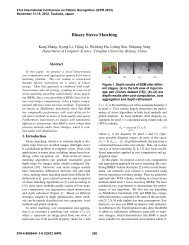
s is set to 0,1,2 or 3 in this paper and the four typical granules are shown in
Fig. 2 (a).
In order to calculate the distance between two granules, Granular space G is
mapped into 3D space I, where for each element g ∈ G and γ ∈ I, g(x, y, s) →
γ(x + 2 s , y + 2 s , 2 s ). The distance between two granules in G is defined to be the
Euclidean distance between two corresponding points in I, d(g 1 , g 2 ) = d(γ 1 , γ 2 )
where g 1 , g 2 ∈ G, γ 1 , γ 2 ∈ I and γ 1 , γ 2 correspond to g 1 , g 2 respectively.
d(γ 1 (x 1 , y 1 , z 1 ), γ 2 (x 2 , y 2 , z 2 )) = √ (x 1 − x 2 ) 2 + (y 1 − y 2 ) 2 + (z 1 − z 2 ) 2 . (2)
3.2 Intra-frame and Inter-frame Comparison Features (I 2 CF s)
Similar to the approach in [1], we consider two frames each time, the previous
one and the latter one, from which two pairs of granules are extracted to fully
capture the appearance and motion features of an object. An I 2 CF can be
represented as a five-tuple c = (mode, g1, i g j 1 , gi 2, g j 2 ), which is also called a cell
according to [5]. The mode is Appearance mode, Difference mode or Consistent
mode. g1, i g j 1 , gi 2 and g j 2 are four granules. The first pair of granules, gi 1 and g j 1
are from the previous frame to describe the appearance of an object. The second
pair of granules, g2 i and g j 2 comes from the previous or latter frame to describe
either appearance or motion information. When the second pair are from the
previous frame, which means that both pairs are from the previous frame, this
kind of feature is Intra-frame Comparison Feature (Intra-frame CF); when
the second pair come from the latter one, the feature becomes Inter-frame
Comparison Feature (Inter-frame CF). Both of these two kinds of comparison
features are combined to be Intra-frame and Inter-frame Comparison Feature
(I 2 CF ).
Appearance mode (A-mode). Pairing Comparison of Color feature (PCC)
is proved to be simple, fast and efficient in [5] . As PCC can describe the invariance
of color to some extent, we extend this idea to 3D space. A-mode compares
two pairs of granules simultaneously:
f A (g i 1, g j 1 , gi 2, g j 2 ) = gi 1 ≥ g j 1 &&gi 2 ≥ g j 2 . (3)
PCC feature is a special case of A-mode. f A (g i 1, g j 1 , gi 2, g j 2 ) = gi 1 ≥ g j 1 , when
g i 1 == g i 2 and g j 1 == gj 2 .
Difference mode (D-mode). D-mode computes the absolute subtractions
of two pairs of granules, defined as:
f D (g1, i g j 1 , gi 2, g j 2 ) = |gi 1 − g2| i ≥ |g j 1 − gj 2 |. (4)

Human Detection in Video over Large Viewpoint Changes 1251
g(2,4,1)
g(3,11,2)
g(16,2,0)
g(10,6,3)
g2
g1
g2
g1
g3
g4
g1
g2
g3
g4
(a)
(b) (c) (d)
Fig. 2: Our proposed I 2 CF . (a) Granular space with four scales (s = 0,1,2,3) of granules
comes from [5]. (b)Two granules g 1 and g 2 connected by a solid line form one pair of
granules applied in APCF [5]. (c) Two pairs of granules are used in each cell of I 2 CF .
The solid line between g 1 and g 2 (or g 3 and g 4) means that g 1 and g 2 (or g 3 and g 4)
come from the same frame. The dashed line connecting g 1 and g 3 (or g 2 and g 4) means
that the locations of g 1 and g 3 (or g 2 and g 4) are related. This relation of locations
is shown in (d). For example, g 3 is in the neighborhood of g 1. This way reduces the
feature pool a lot but still reserves the discriminative weak features.
The motion filters in [1] [2] calculate the difference between one region and
a shifted one by moving it up, left, right or bottom 1 or 2 pixels in the second
frame. There are three main differences between the D-mode and those methods:
1) The restriction for the locations of these regions is defined spatially and much
looser; 2) D-mode considers two pair of regions each time; 3) The only operation
of D-mode is a comparison operator after subtractions.
Consistent-mode (C-mode). C-mode compares the sums of two pairs of
granules to take advantage of consistent information in the appearance of one
frame or successive frames, defined as:
f C (g1, i g j 1 , gi 2, g j 2 ) = (gi 1 + g2) i ≥ (g j 1 + gj 2 ). (5)
C-mode is much simpler and can be quickly calculated compared with 3D
volumetric features [10] and spatial temporal patches [11].
An I 2 CF of length n is represented as {c 0 , c 1 , · · · , c n−1 } and its feature
value is defined as a binary concatenation of corresponding functions of cells in
reverse order as f I2 CF = [b n−1 b n−2 · · · b 2 b 1 ], where b k = f(mode, g i 1, g j 1 , gi 2, g j 2 )
for 0 ≤ k < n.
⎧
⎪⎨ f A (g1, i g j
f(mode, g1, i g j 1 , gi 2, g j 1 , gi 2, g j 2 ), mode = A,
2 ) = f
⎪ D (g1, i g j 1 , gi 2, g j 2 ), mode = D, (6)
⎩
f C (g1, i g j 1 , gi 2, g j 2 ), mode = C.
3.3 Heuristic learning I 2 CF s
Feature reduction. For 58 × 58 samples, there are ∑ 3
s=0 (58 − 2s + 1) × (58 −
2 s +1) = 12239 granules in total and the feature pool contains 3×12239 2 ≃ 6.7×
10 16 weak features without any restrictions, which make the training time and

1252 G. Duan, H. Ai, and S. Lao
memory requirements impractical. With the distance of two granules defined in
Sec. 3.1, two effective constraints are introduced into I 2 CF : 1)Motivated by [5],
the first pair of granules in I 2 CF is constrained as d(g i 1, g j 1 ) ≤ T 1. 2) Considering
of the consistency in one frame or two near video frames, we constrain that the
second pair of granules in I 2 CF is in the neighborhood of the first pair as shown
in Fig. 2 (d):
d(g i 1, g i 2) ≤ T 2 , d(g j 1 , gj 2 ) ≤ T 2. (7)
We set T 1 = 8, T 2 = 4 in our experiments.
Table 1: Learning algorithm of I 2 CF .
Input: Sample set S = {(x i , y i )|1 ≤ i ≤ m} where y i = ±1.
Initialize: Cell space (CS) with all possible cells and empty I 2 CF .
Output: The learned I 2 CF .
Loop:
– Learn the first pair of granules as [5]. Denote the best f pairs as a set F .
– Construct a new set CS’: In each cell of CS’, the first pair of granules is from F , the
second pair of granules is generated by Eq. 7 and its mode is A-mode, D-mode or C-mode.
Calculate Z value of I 2 CF by adding each cell in CS’.
– Select the cell with the lowest Z value, denoted as c ∗ . Add c ∗ to I 2 CF .
– Refine I 2 CF by replacing one or two granules in it without changing the mode.
Heuristically learning I 2 CF starts with an empty I 2 CF . Each time select
the most discriminative cell and add it to I 2 CF . The discriminability of a weak
feature is measured by Z value, which reflects the classification power of the
weak classifier as [17]:
Z = 2 ∑ √
W+W j −, j (8)
j
where W j + is the weight of positive samples that fall into the j th bin while W j −
is that of negatives. The less Z value is, the more discriminative a weak feature
is. The learning algorithm of I 2 CF is summarized in Table 1. (See more details
in [5] [16].)
4 EMC-Boost
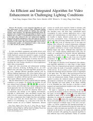
We propose the EMC-Boost to co-cluster the sample space and discriminative
features automatically. A perceptual clustering problem is shown in Fig. 3 (a)-
(c). EMC-Boost consists of three components, Cascade Component (CC), Mixed
Component (MC) and Separated Component (SC). The three components are
combined to become EMC-Boost. In fact, SC is similar to MC-Boost [13], which
is the reason that our boosting algorithm is named as EMC-Boost. In the following
descriptions, we formulate the three components explicitly first, and then
demonstrate the learning algorithms, and summarize EMC-Boost at the end of
this section.

Human Detection in Video over Large Viewpoint Changes 1253
CC
MC
Cluster
(b)
SC
Classifier
(a) (c) (d)
Fig. 3: A perceptual clustering problem in (a)-(c) and a general EMC-Boost in (d)
where CC, MC and SC are three components of EMC-Boost.
4.1 Three components CC/MC/SC
CC deals with a standard 2-class classification problem that can be solved by any
boosting algorithm. MC and SC deal with K clusters. We formulate the detectors
of MC or SC as K strong classifiers, each of which is a linear combination of
weak learners H k (x) = ∑ t α kth kt (x), k = 1, · · · , K with a threshold θ k (default
is 0). Note that the K classifiers H k (x), k = 1, · · · , K are same in MC with K
different thresholds θ k , which means H 1 (x) = H 2 (x) = · · · = H k (x), but they
are totally different in SC. We present MC and SC uniformly below.
The score y ik of the i th sample belonging to the k th clusters can be computed
as y ik = H k (x i )−θ k . Therefore, the probability of x i belonging to the k th cluster
1
is P ik (x) = . For aggregating all scores of one sample on K classifiers,
1+e −y ik
we formulate Noisy-OR like [18] [13] as
P i (x) = 1 −
K∏
(1 − P ik (x i )). (9)
k=1
The cost function is defined as J = ∏ i P ti
i (1 − P i) 1−ti where t i ∈ {0, 1} is
the label of i th sample, which is equivalent to maximize the log-likelihood
log J = ∑ i
t i log P i + (1 − t i ) log(1 − P i ). (10)
4.2 Learning algorithms of CC/MC/SC
The learning algorithm of CC is directly Real Adaboost [17]. The learning algorithm
of MC or SC is different from that of CC. MC and SC learn weak classifiers
to maximize ∑ K ∑
k i w kih kt (x i ) and ∑ i w kih kt (x i ) respectively at t th round of
boosting. Initially, the sample weights are: 1) For positives, w ki = 1 if x i ∈ k and
w ki = 0 otherwise, where i denotes the i th sample and k denotes the k th cluster
or classifier; 2) For all negatives we set w ki = 1/K. Following the AnyBoost
method [19], we set the sample weights as the derivative of the cost function

1254 G. Duan, H. Ai, and S. Lao
w.r.t. the classifier score. The weight of k th classifier over i th sample is updated
by
w ki = ∂ log J
∂y ki
= t i − P i
P i
P ki (x i ). (11)
We sum up the training algorithms of MC and SC in Table 2.
Table 2: Learning algorithms of MC and SC.
Input: Sample set S = {(x i , y i )|1 ≤ i ≤ m} where y i = ±1; Detection rate r in each layer.
Output: H k (x) = P t α kt(x), k = 1, · · · , K.
Loop: For t = 1, · · · , T
(MC)
P
i w kih kt (x i ).
– Find weak classifiers h t, (h kt = h t, k = 1, · · · , K) that maximize P K
k=1
– Find the weak-learner weights α kt , (k = 1, · · · , K) that maximize Γ (H + α kt h kt ).
– Update weights by Eq.11.
(SC) For k = 1, · · · , K
– Find weak classifiers h kt that maximize P i w kih kt (x i ).
– Find the weak-learner weights α kt that maximize Γ (H + α kt h kt ).
– Update weights by Eq.11.
Update thresholds θ k (k = 1, · · · , K) to satisfy detection rate r.
4.3 A general EMC-Boost
The three components of EMC-Boost have different properties. CC takes all
samples as one cluster while MC or SC considers that the whole sample space
consists of multiple clusters. CC tends to distinguish positives from negatives;
while SC tends to cluster the sample space, and MC can do both work at the
same time but not so accurately as CC in classifying positives from negatives
or as SC in clustering. Compared with SC, one particular advantage of MC is
sharing weak features among all clusters. We combine these three components
to become a general EMC-Boost as shown in Fig. 3 (d) which contains five
steps:(Note that Step 2 is similar to CBT [14])
Step 1. CC learns a classifier for all samples considered as one category.
Step 2. K-means algorithm clusters sample space with learned weak features.
Step 3. MC clusters sample space coarsely.
Step 4. SC clusters the sample space further.
Step 5. CC learns a classifier for each cluster center.
5 Multiple Video Sampling
In order to deal with the change in video frame rate or abrupt motion problem,
we introduce a Multiple Video Sampling (MVS) strategy as illustrated in
Fig. 4 (a) and (b). Considering five consecutive frames in (a), a positive sample
is made up of two frames, where one is the first frame and the other is from the

Human Detection in Video over Large Viewpoint Changes 1255
1 2 3 4 5
(a)
1 2 1 3 1 4 1 5
(b)
(c)
Fig. 4: The MVS strategy and some positive samples.
Appearance Motion Appearance+Motion
23.3%
i th cluster
k th cluster
34.9%
15.5%
1 st stage 2 nd stage
(a)
1 st stage 2 nd stage
(b)
10.5%
15.8%
Fig. 5: Two-Stage Tree Structure in (a) and an example in (b). The number in the box
gives the percentage of samples belonging to that branch.
next four frames as shown in (b). In other words, one annotation corresponds to
five consecutive frames and generates 4 positives. Some more positives are shown
in Fig. 4 (c). Suppose that the original frame rate is R and the used positives
consist of the 1 st and the r th frames (r > 1), then the possible frame rate covered
by MVS strategy is R/(r −1). If these positives are extracted from 30 fps videos,
the trained detector is able to deal with 30fps(30/1),15fps(30/2),10fps(30/3) and
7.5fps(30/4) videos where r is 2, 3, 4 and 5 respectively.
6 Overview of Our Approach
We adopt EMC-Boost selecting I 2 CF as weak features to learn a strong classifier
for multiple viewpoint human detection, in which positive samples are achieved
through MVS strategy. Due to the large amount of samples and features, it is
difficult to learn a detector directly by a general EMC-Boost. We modify the
detector structure slightly and propose a new structure containing two stages
as shown in Fig. 5 (a) with an example in (b), which is called two-stage tree
structure: In the 1 st stage, it only uses appearance information for learning and
clustering; In the 2 nd stage, it uses both appearance and motion information for
clustering first, and then for learning classifiers for all clusters.
7 Experiments
We carry out some experiments to evaluate our approach by False Positive Per
Image (FPPI) on several real-world challenging datasets, ETHZ, PET2007 and
our own collected dataset. When the intersection between a detection response

1256 G. Duan, H. Ai, and S. Lao
and a ground-truth box is larger than 50% of their union, we consider it to be
a successful detection. Only one detection per annotation is counted as correct.
For simplicity, the three typical viewpoints mentioned in Fig. 1 are represented
as Horizontal Viewpoint (HV), Slant Viewpoint (SV) and Vertical Viewpoint
(VV) in turn from left to right.
Datasets. The datasets used in the experiments are ETHZ dataset [20],
PETS2007 dataset [21] and our own collected dataset. ETHZ dataset provides
four video sequences, Seq.#0∼Seq.#3 (640×480 pixels at 15 fps). This dataset
whose viewpoint is near HV is recorded using a pair of cameras, and we only use
the images provided by the left camera. PETS2007 dataset contains 9 sequences
S00∼S08 (720×576 pixels at 30 fps) and each sequence has 4 fixed cameras and
we choose the 3 rd camera whose viewpoint is near SV. There are 3 scenarios in
PETS2007, with increasing scene complexity, loitering (S01 and S02), attended
luggage removal (S03, S04, S05 and S06) and unattended luggage (S07 and S08).
In the experiments, we use S01, S03, S05 and S06. In addition, we have collected
several sequences by hand-held DV cameras: 2 sequences near HV (853×480
pixels at 30 fps), and 2 sequences near SV (1280×720 pixels at 30 fps) and 8
sequences near VV (2 sequences are 1280×720 pixels at 30 fps and the others
are 704×576 pixels at 30 fps).
Training and testing datasets. S01, S03, S05 and S06 of PETS2007 and
our own dataset are labeled every five frames manually for training and testing,
while ETHZ dataset provides the groundtruth already. The training datasets
contain Seq.#0 of ETHZ, S01, S03 and S06 of PETS2007, 2 sequences (near HV),
2 sequences (near SV) and 6 sequences (near VV) of ours. The testing datasets
contain Seq.#1, Seq.#2 and Seq.#3 of ETHZ, S05 of PETS2007, and 2 sequences
of ours (near VV). Note that the groundtruths of the internal unlabeled frames
in the testing datasets are achieved through interpolation. The properties of the
testing datasets may have impacts on all detectors, like camera motion states
(fixed or moving), illumination conditions (slightly or significantly light changes),
etc. Details about the testing datasets are summarized in Table 3.
Training detectors. We have labeled 11768 different humans in total and
obtain 47072 positives after MVS, where the number of positives near HV, SV
Table 3: Some details about the testing datasets.
Description Seq. 1 Seq. 2 S05 Seq.#1 Seq.#2 Seq.#3
Source ours ours PETS2007 ETHZ ETHZ ETHZ
Camera Fixed Fixed Fixed Moving Moving Moving
Light changes Slightly Slightly Slightly Slightly Slightly Significantly
Frame rate 30fps 30fps 30fps 15fps 15fps 15fps
Size 704×576 704×576 720×576 640×480 640×480 640×480
Frames 2420 1781 4500 999 450 354
Annotations 591 1927 17067 5193 2359 1828

Reca l
Reca l
Reca l
Reca l
Reca l
Reca l
Human Detection in Video over Large Viewpoint Changes 1257
0.95
Test Sequence 1 (ours, 2420 frames, 591 annotations)
0.9
Test Sequence 2 (ours, 1718 frames, 1927 annotations)
0.9
0.85
0.85
0.8
0.8
0.75
0.75
0.7
0.05 0.1 0.15 0.2 0.25 0.3
FPPI
0.75
Intra-frame CF + Boost
Intra-frame CF + EMC-Boost
I 2 CF + EMC-Boost
S05 (PETS2007, 4500 frames, 17067 annotations)
0.7
Intra-frame CF + Boost
Intra-frame CF + EMC-Boost
I 2 CF + EMC-Boost
0.65
0.2 0.4 0.6 0.8 1 1.2 1.4 1.6 1.8 2
FPPI
0.8
Seq. #1 (ETHZ, 999 frames, 5193 annotations)
0.7
0.65
0.75
0.7
0.65
0.6
0.6
0.55
0.55
0.5
0.5
0.45
Ess et al.
Schwartz et al.
0.45
Intra-frame CF + Boost
Intra-frame CF + EMC-Boost
I 2 CF + EMC-Boost
0.4
0.35
Wojek et al.(HOG, IMHwd and HIKSVM)
Intra-frame CF + Boost
Intra-frame CF + EMC-Boost
I 2 CF + EMC-Boost
0.4
0.2 0.4 0.6 0.8 1 1.2 1.4 1.6 1.8 2
FPPI
0.75
0.7
0.65
0.6
Seq. #2 (ETHZ, 450 frames, 2359 annotations)
0 1 2 3 4 5 6
FPPI
Seq. #3 (ETHZ, 354 frames, 1828 annotations)
0.9
0.8
0.7
0.55
0.6
0.5
0.45
Ess et al.
Schwartz et al.
0.4
Wojek et al.(HOG, IMHwd and HIKSVM)
Intra-frame CF + Boost
0.35
Intra-frame CF + EMC-Boost
I 2 CF + EMC-Boost
0 0.5 1 1.5 2 2.5 3 3.5 4
FPPI
0.5
0.4
0.3
Ess et al.
Schwartz et al.
Wojek et al.(HOG, IMHwd and HIKSVM)
Intra-frame CF + Boost
Intra-frame CF + EMC-Boost
I 2 CF + EMC-Boost
0.2
0 0.5 1 1.5 2 2.5 3 3.5 4
FPPI
Fig. 6: Evaluation of our approach and some results.
and VV are 18976, 19248 and 8848 respectively. The size of positives is normalized
to 58 × 58. Some positives are shown in Fig. 4. We train a detector based on
EMC-Boost selecting I 2 CF as features. Implementation details. We cluster the
sample space into 2 clusters in the 1 st stage and cluster the two sub spaces into
2 and 3 clusters separately in the 2 nd stage as illustrated in Fig. 5 (b). When do
we start and stop MC/SC? When the false positive rate is less than 10 −2 (10 −4 )
in the 1 st (2 nd ) stage, we start MC and then start SC after learning by MC.
Before describing when to stop MC or SC, we first define transferred samples. A
sample is called transferred if it belongs to another cluster after current round
boosting. We stop MC (SC) when the number of transferred samples is less than
10% (2%) of the total number of samples.
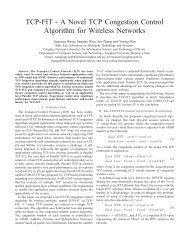
Evaluation. To compare with our approach (denoted as I 2 CF +EMC-Boost),
two other detectors are trained: one is to adopt Intra-frame CF learned by a general
Boost algorithm like [5] [15] (denoted as Intra-frame CF+Boost) and the
other one is to adopt Intra-frame CF learned by EMC-Boost (denoted as Intraframe
CF+EMC-Boost). Note that due to the large amount of Inter-frame CFs,
the large amount of positives and memory limited, it is impractical to learn a
detector of Inter-frame CF by Boost or EMC-Boost.
We compare our approach with Intra-frame CF + Boost and Intra-frame CF
+ EMC-Boost approaches on PETS2007 dataset and our own collected videos,
and also with [4] [20] [22] on ETHZ dataset. We give the ROC curves and some
results in Fig. 6. In general, our proposed approach which integrates appearance
and motion information is superior to Intra-frame CF+Boost and Intra-frame
CF+EMC-Boost approaches which only use appearance information. From another
viewpoint, this experiment also indicates that incorporating motion information
improves detection significantly as [4].

Recall
Recall
Recall
Recall
Recall
Recall
1258 G. Duan, H. Ai, and S. Lao
1
Test Sequence 1 of ours
1
Test Sequence 2 of ours
0.75
S05 of PETS2007
0.95
0.95
0.7
0.9
0.9
0.65
0.85
0.85
0.6
0.8
0.75
0.7
0.65
0.05 0.1 0.15 0.2 0.25 0.3
FPPI
1
1/2
1/3
1/4
1/5
0.8
0.75
0.7
1
1/2
1/3
0.65
1/4
1/5
0.2 0.4 0.6 0.8 1 1.2 1.4 1.6
FPPI
0.55
0.5
0.45
0.4
0.2 0.4 0.6 0.8 1 1.2 1.4 1.6
FPPI
1
1/2
1/3
1/4
1/5
0.7
Seq.#1 of ETHZ
0.9
Seq.#2 of ETHZ
0.8
Seq.# 3 of ETHZ
0.65
0.8
0.75
0.6
0.7
0.55
0.7
0.65
0.5
0.6
0.6
0.55
0.45
0.5
0.5
0.4
0.35
0.3
0.25
0.2 0.4 0.6 0.8 1 1.2 1.4 1.6 1.8 2 2.2
FPPI
1
1/2
1/3
1/4
1/5
0.4
0.3
0.2
0 0.2 0.4 0.6 0.8 1 1.2 1.4 1.6
FPPI
1
1/2
1/3
1/4
1/5
0.45
1
0.4
1/2
1/3
0.35
1/4
1/5
0 0.2 0.4 0.6 0.8 1 1.2 1.4 1.6 1.8 2
FPPI
Fig. 7: The robustness evaluation of our approach to video frame rate changes. 1 represents
the original frame rate, 1/2 represents that the testing dataset is downsampled
to 1/2 original frame rate and so as 1/3, 1/4 and 1/5.
Compared to [20] [22], our approach is better. Furthermore, we have not used
any additional cues like depth maps, ground-plane estimation, and occlusion reasoning,
which are used in [20]. “HOG, IMHwd and HIKSVM” proposed in [4],
combines HOG feature [18] and the Internal Motion Histogram wavelet difference
(IMHwd) descriptor [3] together using histogram intersection kernel SVM
(HIKSVM) and achieves the best results than other approaches used in [4]. Our
approach is not as good as but comparable to “ HOG, IMHwd and HIKSVM”and
we argue that our approach is much simpler and faster. Currently, our approach
takes about 0.29s on ETHZ, 0.61s on PETS and 0.55s on our dataset to process
one frame in average.
In order to evaluate the robustness of our approach to video frame rate
changes, we downsample the videos to their 1/2, 1/3, 1/4 and 1/5 original frame
rate to compare with the original frame rate. Our approach is evaluated on
the testing datasets with frame rate changes, and the ROC curves are shown in
Fig. 7. The results on the three sequences of ETHZ dataset and S05 of PETS2007
are similar, but the results on our collected two sequences differ a lot. The main
reason is that: 1) as frame rates get lower, human motion changes more abruptly;
2) note that human motion in near VV videos changes more fiercely than that
in near HV or SV ones. Our collected two sequences are near VV, so relatively
human motion changes even more drastically than the other testing datasets.
Generally speaking, our approach is robust to the video frame rate change to a
certain extent.
Discussions. We then discuss about the selection of EMC-Boost instead of
MC-Boost and a general Boost algorithm.
MC-Boost runs several classifiers together at any time, which may be good at
classification problems, but not at detection problems. Considering the sharing

Human Detection in Video over Large Viewpoint Changes 1259
feature at the beginning of clustering and the good clusters after clustering, we
propose more suitable learning algorithms, MC and SC, for detection problems.
Furthermore, risk map is an essential part of MC-Boost, in which the risk of one
sample is related to predefined neighbors in the same class and in the opposite.
But a proper neighborhood definition itself might be a tough question. For preserving
the merits of MC-Boost and avoiding its shortcomings, we argue that
EMC-Boost is more suitable for a detection problem.
A general Boost algorithm can work well when the sample space has fewer
variations, while EMC-Boost is designed to cluster the space into several sub
ones which can make the learning process faster. But after clustering, a sample
is considered as correct if it belongs to any sub space and thus it may also bring
with more negatives. This may be the reason that Intra-frame CF+EMC-Boost
is inferior to Intra-frame CF+Boost in Fig. 6. Mainly considering the cluster
ability, we choose EMC-Boost other than a general Boost algorithm. In fact, it
is impractical to learn a detector of I 2 CF +Boost without clustering because of
the large amount of weak features and positives.
8 Conclusion
In this paper, we propose Intra-frame and Inter-frame Comparison Features
(I 2 CF s), Enhanced Multiple Clusters Boost algorithm (EMC-Boost), Multiple
Video Sampling (MVS) strategy and a two-stage tree structure detector to detect
human in video over large viewpoint change. I 2 CF s combine appearance
information and motion information automatically. EMC-Boost can cluster a
sample space quickly and efficiently. MVS strategy makes our approach robust
to frame rate and human motion. The final detector is organized as a two-stage
tree structure to fully mine the discriminative features of the appearance and
motion information. The evaluations on challenging datasets show the efficiency
of our approach.
There are some future works to be done. The large feature pool causes lots
of difficulties during training. One work is to design a more efficient learning
algorithm. MVS strategy can make the approach more robust to frame rate,
but not handle arbitrary frame rates once a detector is learned. To achieve
better results, another work may integrate object detection in video with object
detection in static images and object tracking. An interesting question to EMC-
Boost is what kind of clusters EMC-Boost can obtain. Take human for example.
Different poses, views, viewpoints or illumination will make human different and
perceptual co-clusters of these samples differ with different criterion. The further
relation between the discriminative features and samples is critical to the results.
Another work may study the relations among features, objects and EMC-Boost.
Our approach can also be applied to other object detection, multiple objects
detection or object category as well.
Acknowledgement. This work is supported by National Science Foundation of
China under grant No.61075026, and it is also supported by a grant from Omron
Corporation.

1260 G. Duan, H. Ai, and S. Lao
References
1. Viola, P., Jones, M., Snow, D.: Detecting pedestrians using patterns of motion
and appearance. In: IEEE International Conference on Computer Vision (ICCV).
(2003)
2. Jones, M., Snow, D.: Pedestrian detection using boosted features over many frames.
In: International Conference on Pattern Recognition (ICPR), Motion, Tracking,
Video Analysis. (2008)
3. Dalal, N., Triggs, B., Schmid, C.: Human detection using oriented histograms of
flow and appearance. In: ECCV. (2006)
4. Wojek, C., Walk, S., Schiele, B.: Multi-cue onboard pedestrian detection. In:
CVPR. (2009)
5. Duan, G., Huang, C., Ai, H., Lao, S.: Boosting associated pairing comparison
features for pedestrian detection. In: 9th Workshop on Visual Surveillance. (2009)
6. Dalal, N., Triggs, B.: Histograms of oriented gradients for human detection. In:
CVPR. (2005)
7. Wu, B., Nevatia, R.: Detection of multiple, partially occluded humans in a single
image by bayesian combination of edgelet part detectors. In: ICCV. (2005)
8. Yang, M., Yuan, J., Wu, Y.: Spatial selection for attentional visual tracking. In:
CVPR. (2007)
9. Andriluka, M., Roth, S., Schiele, B.: People-tracking-by-detection and peopledetection-by-tracking.
In: CVPR. (2008)
10. Ke, Y., Sukthankar, R., Hebert, M.: Efficient visual event detection using volumetric
features. In: ICCV. (2005)
11. Shechtman, E., Irani, M.: Space-time behavior based correlation. In: CVPR. (2005)
12. Jordan, M., Jacobs, R.: Hierarchical mixture of experts and the em algorithm.
Neural Computation 6 (1994) 181–214
13. Kim, T.K., Cipolla, R.: Mcboost: Multiple classifier boosting for perceptual coclustering
of images and visual features. In: Advances in Neural Information Processing
Systems (NIPS). (2008)
14. Wu, B., Nevatia, R.: Cluster boosted tree classifier for multi-view, multi-pose
object detection. In: ICCV. (2007)
15. Viola, P., Jones, M.: Rapid object detection using a boosted cascade of simple
features. In: CVPR. (2001)
16. HUANG, C., AI, H., LI, Y., LAO, S.: Learning sparse features in granular space
for multi-view face detection. In: IEEE International Conference, Automatic Face
and Gesture Recognition. (2006)
17. Schapire, R.E., Singer, Y.: Improved boosting algorithms using confidence-rated
predictions. Machine Learning 37 (1999) 297–336
18. Viola, P., Platt, J., Zhang, C.: Multiple instance boosting for object detection. In:
NIPS. (2005)
19. Mason, L., Baxter, J., Bartlett, P., Frean, M.: Boosting algorithms as gradient
descent. In: Proc. Advances in Neural Information Processing Systems. (2000)
20. Ess, A., Leibe, B., Gool, L.V.: Depth and appearance for mobile scene analysis.
In: ICCV. (2007)
21. PETS2007. (http://www.cvg.rdg.ac.uk/PETS2007/)
22. Schwartz, W.R., Kembhavi, A., Harwood, D., Davis, L.S.: Human detection using
partial least squares analysis. In: ICCV. (2009)