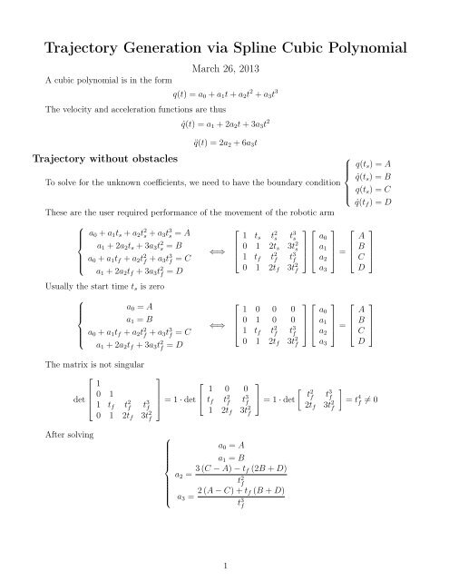
Trajectory Generation via Spline Cubic Polynomial

Trajectory Generation via Spline Cubic Polynomial
A cubic polynomial is in the form
March 26, 2013
q(t) = a 0 + a 1 t + a 2 t 2 + a 3 t 3
The velocity and acceleration functions are thus
Trajectory without obstacles
˙q(t) = a 1 + 2a 2 t + 3a 3 t 2
¨q(t) = 2a 2 + 6a 3 t
⎧
q(t s ) = A
⎪⎨
˙q(t s ) = B
To solve for the unknown coefficients, we need to have the boundary condition
q(t s ) = C
⎪⎩
˙q(t f ) = D
These are the user required performance of the movement of the robotic arm
⎧
⎪⎨
⎪⎩
a 0 + a 1 t s + a 2 t 2 s + a 3 t 3 s = A
a 1 + 2a 2 t s + 3a 3 t 2 s = B
a 0 + a 1 t f + a 2 t 2 f + a 3t 3 f = C
a 1 + 2a 2 t f + 3a 3 t 2 f = D
Usually the start time t s is zero
⎧
⎪⎨
⎪⎩
a 0 = A
a 1 = B
a 0 + a 1 t f + a 2 t 2 f + a 3t 3 f = C
a 1 + 2a 2 t f + 3a 3 t 2 f = D
⇐⇒
⇐⇒
⎡
⎢
⎣
⎡
⎢
⎣
1 t s t 2 s t 3 s
0 1 2t s 3t 2 s
1 t f t 2 f t 3 f
0 1 2t f 3t 2 f
1 0 0 0
0 1 0 0
1 t f t 2 f t 3 f
0 1 2t f 3t 2 f
⎤ ⎡ ⎤ ⎡
a 0
⎥ ⎢ a 1
⎥
⎦ ⎣ a 2
⎦ = ⎢
⎣
a 3
⎤ ⎡ ⎤ ⎡
a 0
⎥ ⎢ a 1
⎥
⎦ ⎣ a 2
⎦ = ⎢
⎣
a 3
A
B
C
D
A
B
C
D
⎤
⎥
⎦
⎤
⎥
⎦
The matrix is not singular
⎡
1
det ⎢ 0 1
⎣ 1 t f t 2 f t 3 f
0 1 2t f 3t 2 f
⎤
⎡
⎥
⎦ = 1 · det ⎣
1 0 0
t f t 2 f t 3 f
1 2t f 3t 2 f
⎤
⎦ = 1 · det
[ t
2
f t 3 f
2t f 3t 2 f
]
= t 4 f ≠ 0
After solving
⎧
⎪⎨
⎪⎩
a 0 = A
a 1 = B
a 2 = 3 (C − A) − t f (2B + D)
t 2 f
a 3 = 2 (A − C) + t f (B + D)
t 3 f
1

And thus the equation ( displacement, velocity and acceleration ) are
⎧
⎪⎨
⎪⎩
q(t) = A + Bt + 3 (C − A) − t f (2B + D)
t 2 f
˙q(t) = B + 6 (C − A) − 2t f (2B + D)
t 2 f
¨q(t) = 6 (C − A) − 2t f (2B + D)
t 2 f
t 2 + 2 (A − C) + t f (B + D)
t 3
t 3 f
t + 6 (A − C) + 3t f (B + D)
t 2
t 3 f
+ 12 (A − C) + 6t f (B + D)
t
t 3 f
Since usually the initial and final velocity is zero ( stop at both end ), thus in these cases B = D = 0
, and the eqaution reduce to
⎧
⎪⎨
⎪⎩
Trajectory with obstacles
3 (C − A)
q(t) = A + t 2 2 (A − C)
+
˙q(t) =
¨q(t) =
t 2 f
t 3 f
6 (C − A) 6 (A − C)
t +
t 2 f
6 (C − A)
t 2 f
+
t 3 f
t 2
12 (A − C)
t
t 3 f
When the trajectory need to avoid some obstacles, that means the trajectory should not pass through
some points.
To make it simple, that means the trajectory should pass through some points that can avoid hitting
the obstacles.
t 3
Suppose in addition to the upper part, now the trajectory has to pass throguh points p 1 at time t p
How to determine the unknown velocity ?
starting point p s p 1 end point p e
displacement known given known
velocity zero ? zero
The most simple idea is to choose the velocity ( they are free variable ) that the acceleration is
continuous in these point.
As acceleration means force, and a drag force that suddenly appear is not good for robotic arm.
Thus first , split the path from one to 2 path
Original path is p s → p e , now p s → p 1 → p e
{
a 0 + a 1 t + a 2 t 2 + a 3 t 3 t ∈ [t s , t p ]
Since there are 2 path, that means there is 2 displacement equations
b 0 + b 1 t + b 2 t 2 + b 3 t 3 t ∈ [t p , t e ]
Let the velocity at time t p be v
Solve the 2 equations, and equal the acceleration equations to solve for the unknowns.
−END−
2