

Relativistic Quantum Mechanics - Theory of Condensed Matter
Relativistic Quantum Mechanics - Theory of Condensed Matter
Relativistic Quantum Mechanics - Theory of Condensed Matter

You also want an ePaper? Increase the reach of your titles
YUMPU automatically turns print PDFs into web optimized ePapers that Google loves.
Chapter 15<br />
<strong>Relativistic</strong> <strong>Quantum</strong><br />
<strong>Mechanics</strong><br />
The aim <strong>of</strong> this chapter is to introduce and explore some <strong>of</strong> the simplest aspects<br />
<strong>of</strong> relativistic quantum mechanics. Out <strong>of</strong> this analysis will emerge the Klein-<br />
Gordon and Dirac equations, and the concept <strong>of</strong> quantum mechanical spin.<br />
This introduction prepares the way for the construction <strong>of</strong> relativistic quantum<br />
field theories, aspects touched upon in our study <strong>of</strong> the quantum mechanics<br />
<strong>of</strong> the EM field. To prepare our discussion, we begin first with a survey <strong>of</strong><br />
the motivations to seek a relativistic formulation <strong>of</strong> quantum mechanics, and<br />
some revision <strong>of</strong> the special theory <strong>of</strong> relativity.<br />
Why study relativistic quantum mechanics? Firstly, there are many experimental<br />
phenomena which cannot be explained or understood within the<br />
purely non-relativistic domain. Secondly, aesthetically and intellectually it<br />
would be pr<strong>of</strong>oundly unsatisfactory if relativity and quantum mechanics could<br />
not be united. Finally there are theoretical reasons why one would expect new<br />
phenomena to appear at relativistic velocities.<br />
When is a particle relativistic? Relativity impacts when the velocity approaches<br />
the speed <strong>of</strong> light, c or, more intrinsically, when its energy is large<br />
compared to its rest mass energy, mc 2 . For instance, protons in the accelerator<br />
at CERN are accelerated to energies <strong>of</strong> 300GeV (1GeV= 10 9 eV) which is<br />
considerably larger than their rest mass energy, 0.94 GeV. Electrons at LEP<br />
are accelerated to even larger multiples <strong>of</strong> their energy (30GeV compared to<br />
5 × 10 −4 GeV for their rest mass energy). In fact we do not have to appeal to<br />
such exotic machines to see relativistic effects – high resolution electron microscopes<br />
use relativistic electrons. More mundanely, photons have zero rest<br />
mass and always travel at the speed <strong>of</strong> light – they are never non-relativistic.<br />
What new phenomena occur? To mention a few:<br />
⊲ Particle production: One <strong>of</strong> the most striking new phenomena to<br />
emerge is that <strong>of</strong> particle production – for example, the production <strong>of</strong><br />
electron-positron pairs by energetic γ-rays in matter. Obviously one<br />
needs collisions involving energies <strong>of</strong> order twice the rest mass energy <strong>of</strong><br />
the electron to observe production.<br />
Astrophysics presents us with several examples <strong>of</strong> pair production. Neutrinos<br />
have provided some <strong>of</strong> the most interesting data on the 1987 supernova.<br />
They are believed to be massless, and hence inherently relativistic;<br />
moreover the method <strong>of</strong> their production is the annihilation <strong>of</strong><br />
electron-positron pairs in the hot plasma at the core <strong>of</strong> the supernova.<br />
High temperatures, <strong>of</strong> the order <strong>of</strong> 10 12 K are also inferred to exist in the<br />
nuclei <strong>of</strong> some galaxies (i.e. k B T ≫ 2mc 2 ). Thus electrons and positrons<br />
Advanced <strong>Quantum</strong> Physics
168<br />
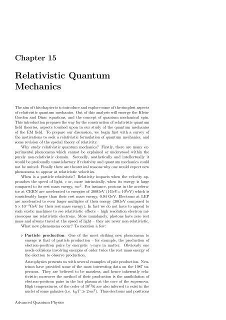
Figure 15.1: Anderson’s cloud chamber picture <strong>of</strong> cosmic radiation from 1932 showing<br />
for the first time the existence <strong>of</strong> the positron. A cloud chamber contains a gas<br />
supersaturated with water vapour (left). In the presence <strong>of</strong> a charged particle (such<br />
as the positron), the water vapour condenses into droplets – these droplets mark out<br />
the path <strong>of</strong> the particle. In the picture a charged particle is seen entering from the<br />
bottom at high energy. It then looses some <strong>of</strong> the energy in passing through the 6 mm<br />
thick lead plate in the middle. The cloud chamber is placed in a magnetic field and<br />
from the curvature <strong>of</strong> the track one can deduce that it is a positively charged particle.<br />
From the energy loss in the lead and the length <strong>of</strong> the tracks after passing though the<br />
lead, an upper limit <strong>of</strong> the mass <strong>of</strong> the particle can be made. In this case Anderson<br />
deduces that the mass is less that two times the mass <strong>of</strong> the electron. Carl Anderson<br />
(right) won the 1936 Nobel Prize for Physics for this discovery. (The cloud chamber<br />
track is taken from C. D. Anderson, The positive electron, Phys. Rev. 43, 491 (1933).<br />
are produced in thermal equilibrium like photons in a black-body cavity.<br />
Again a relativistic analysis is required.<br />
⊲ Vacuum instability: Neglecting relativistic effects, we have shown that<br />
the binding energy <strong>of</strong> the innermost electronic state <strong>of</strong> a nucleus <strong>of</strong> charge<br />
Z is given by,<br />
( ) Ze<br />
2 2 m<br />
E = −<br />
4πɛ 0 2 2 .<br />
If such a nucleus is created without electrons around it, a peculiar phenomenon<br />
occurs if |E| > 2mc 2 . In that case, the total change in energy<br />
<strong>of</strong> producing an electron-positron pair, subsequently binding the electron<br />
in the lowest state and letting the positron escape to infinity (it<br />
is repelled by the nucleus), is negative. There is an instability! The<br />
attractive electrostatic energy <strong>of</strong> binding the electron pays the price <strong>of</strong><br />
producing the pair. Nuclei with very high atomic mass spontaneously<br />
“screen” themselves by polarising the vacuum via electron-positron production<br />
until the they lower their charge below a critical value Z c . This<br />
implies that objects with a charge greater than Z c are unobservable due<br />
to screening.<br />
⊲ Info. An estimate based on the non-relativistic formula above gives Z c ≃<br />
270. Taking into account relativistic effects, the result is renormalised downwards<br />
to 137, while taking into account the finite size <strong>of</strong> the nucleus one finally<br />
obtains Z c ∼ 165. Of course, no such nuclei exist in nature, but they can be<br />
manufactured, fleetingly, in uranium ion collisions where Z =2× 92 = 184.<br />
Indeed, the production rate <strong>of</strong> positrons escaping from the nucleus is seen to<br />
increase dramatically as the total Z <strong>of</strong> the pair <strong>of</strong> ions passes 160.<br />
⊲ Spin: Finally, while the phenomenon <strong>of</strong> electron spin has to be grafted<br />
Advanced <strong>Quantum</strong> Physics
169<br />
artificially onto the non-relativistic Schrödinger equation, it emerges naturally<br />
from a relativistic treatment <strong>of</strong> quantum mechanics.<br />
When do we expect relativity to intrude into quantum mechanics? According<br />
to the uncertainty relation, ∆x∆p ≥ /2, the length scale at which the<br />
kinetic energy is comparable to the rest mass energy is set by the Compton<br />
wavelength<br />
∆x ≥ h mc ≡ λ c.<br />
We may expect relativistic effects to be important if we examine the motion<br />
<strong>of</strong> particles on length scales which are less than λ c . Note that for particles <strong>of</strong><br />
zero mass, λ c = ∞! Thus for photons, and neutrinos, relativity intrudes at<br />
any length scale.<br />
What is the relativistic analogue <strong>of</strong> the Schrödinger equation? Non-relativistic<br />
quantum mechanics is based on the time-dependent Schrödinger equation<br />
Ĥψ = i∂ t ψ, where the wavefunction ψ contains all information about a given<br />
system. In particular, |ψ(x, t)| 2 represents the probability density to observe a<br />
particle at position x and time t. Our aim will be to seek a relativistic version<br />
<strong>of</strong> this equation which has an analogous form. The first goal, therefore, is to<br />
find the relativistic Hamiltonian. To do so, we first need to revise results from<br />
Einstein’s theory <strong>of</strong> special relativity:<br />
⊲ Info. Lorentz Transformations and the Lorentz Group: In the special<br />
theory <strong>of</strong> relativity, a coordinate in space-time is specified by a 4-vector. A contravariant<br />
4-vector x =(x µ ) ≡ (x 0 ,x 1 ,x 2 ,x 3 ) ≡ (ct, x) is transformed into the<br />
covariant 4-vector x µ = g µν x ν by the Minkowskii metric<br />
⎛<br />
⎞<br />
1<br />
⎜ −1 ⎟<br />
(g µν )= ⎝<br />
⎠ , gµ ν g<br />
−1<br />
νλ = δ µλ ,<br />
−1<br />
Here, by convention, summation is assumed over repeated indicies. Indeed, summation<br />
covention will be assumed throughout this chapter. The scalar product <strong>of</strong><br />
4-vectors is defined by<br />
x · y = x µ y µ = x µ y ν g µν = x µ y µ .<br />
The Lorentz group consists <strong>of</strong> linear Lorentz transformations, Λ, preserving x·y,<br />
i.e. for x µ ↦→ x ′µ =Λ µ νx ν , we have the condition<br />
g µν Λ µ αΛ ν β = g αβ . (15.1)<br />
Specifically, a Lorentz transformation along the x 1 direction can be expressed in the<br />
form<br />
⎛<br />
⎞<br />
γ −γv/c<br />
Λ µ ⎜ −γv/c γ ⎟<br />
ν = ⎝<br />
⎠<br />
1 0<br />
0 1<br />
where γ = (1 − v 2 /c 2 ) −1/2 . 1 With this definition, the Lorentz group splits up into<br />
four components. Every Lorentz transformation maps time-like vectors (x 2 > 0) into<br />
1 Equivalently the Lorentz transformation can be represented in the form<br />
0<br />
1<br />
0 −1<br />
Λ = exp[ωK 1], [K 1] µ ν = B −1 0<br />
C<br />
@ 0 0A ,<br />
0 0<br />
where ω = tanh −1 (v/c) is known as the rapidity, and K 1 is the generator <strong>of</strong> velocity<br />
transformations along the x 1-axis.<br />
Advanced <strong>Quantum</strong> Physics
15.1. KLEIN-GORDON EQUATION 170<br />
time-like vectors. Time-like vectors can be divided into those pointing forwards in<br />
time (x 0 > 0) and those pointing backwards (x 0 < 0). Lorentz transformations do<br />
not always map forward time-like vectors into forward time-like vectors; indeed Λ<br />
does so if and only if Λ 0 0 > 0. Such transformations are called orthochronous.<br />
(Since Λ µ 0 Λ µ0 = 1, (Λ 0 0) 2 − (Λ j 0 )2 = 1, and so Λ 0 0 ≠ 0.) Thus the group splits<br />
into two according to whether Λ 0 0 > 0 or Λ 0 0 < 0. Each <strong>of</strong> these two components<br />
may be subdivided into two by considering those Λ for which det Λ = ±1. Those<br />
transformations Λ for which det Λ = 1 are called proper.<br />
Thus the subgroup <strong>of</strong> the Lorentz group for which det Λ = 1 and Λ 0 0 > 0 is<br />
called the proper orthochronous Lorentz group, sometimes denoted by L ↑ +. It<br />
contains neither the time-reversal nor parity transformation,<br />
⎛<br />
⎞ ⎛<br />
⎞<br />
−1<br />
1<br />
T =<br />
⎜<br />
⎝<br />
1<br />
1<br />
⎟ ⎜<br />
⎠ , P = ⎝<br />
1<br />
−1<br />
−1<br />
−1<br />
⎟<br />
⎠ . (15.2)<br />
We shall call it the Lorentz group for short and specify when we are including T or P .<br />
In particular, L ↑ +, L ↑ = L ↑ + ∪L ↑ − (the orthochronous Lorentz group), L + = L ↑ + ∪L ↓ +<br />
(the proper Lorentz group), and L 0 = L ↑ + ∪L ↓ − are subgroups, while L ↓ − = P L ↑ +,<br />
L ↑ − = T L ↑ + and L ↓ + = TPL ↑ + are not.<br />
Special relativity requires that theories should be invariant under Lorentz transformations<br />
x µ ↦−→ Λ µ νx ν , and, more generally, Poincaré transformations x µ →<br />
Λ µ νx ν + a µ . The proper orthochronous Lorentz transformations can be reached continuously<br />
from identity. 2 Loosely speaking, we can form them by putting together<br />
infinitesimal Lorentz transformations Λ µ ν = δ µ ν +ω µ ν, where the elements <strong>of</strong> ω µ ν ≪ 1.<br />
Applying the identity g αβ =Λ µ αΛ µβ = g αβ + ω αβ + ω βα + O(ω 2 ), we obtain the<br />
relation ω αβ = −ω βα . ω αβ has six independent components: L ↑ + is a six-dimensional<br />
(Lie) group, i.e. it has six independent generators: three rotations and three boosts.<br />
Finally, according to the definition <strong>of</strong> the 4-vectors, the covariant and contravariant<br />
derivative are respectively defined by ∂ µ = ∂<br />
∂x<br />
= ( 1 ∂<br />
µ c ∂t , ∇), ∂µ = ∂<br />
∂x µ<br />
=<br />
( 1 ∂<br />
c ∂t<br />
, −∇). Applying the scalar product to the derivative we obtain the d’Alembertian<br />
operator (sometimes denoted as ✷), ∂ 2 = ∂ µ ∂ µ = 1 ∂ 2<br />
c 2 ∂t<br />
−∇ 2 .<br />
2<br />
15.1 Klein-Gordon equation<br />
Historically, the first attempt to construct a relativistic version <strong>of</strong> the Schrödinger<br />
equation began by applying the familiar quantization rules to the relativistic<br />
energy-momentum invariant. In non-relativistic quantum mechanics the correspondence<br />
principle dictates that the momentum operator is associated with<br />
the spatial gradient, ˆp = −i∇, and the energy operator with the time derivative,<br />
Ê = i∂ t . Since (p µ ≡ (E/c, p) transforms like a 4-vector under Lorentz<br />
transformations, the operator ˆp µ = i∂ µ is relativistically covariant.<br />
Non-relativistically, the Schrödinger equation is obtained by quantizing<br />
the classical Hamiltonian. To obtain a relativistic version <strong>of</strong> this equation,<br />
one might apply the quantization relation to the dispersion relation obtained<br />
from the energy-momentum invariant p 2 =(E/c) 2 − p 2 =(mc) 2 , i.e.<br />
E(p) =+ ( m 2 c 4 + p 2 c 2) 1/2<br />
⇒<br />
i∂ t ψ = [ m 2 c 4 − 2 c 2 ∇ 2] 1/2<br />
ψ<br />
where m denotes the rest mass <strong>of</strong> the particle. However, this proposal poses<br />
a dilemma: how can one make sense <strong>of</strong> the square root <strong>of</strong> an operator? Interpreting<br />
the square root as the Taylor expansion,<br />
i∂ t = mc 2 ψ − 2 ∇ 2<br />
2m ψ − 4 (∇ 2 ) 2<br />
8m 3 c 2 ψ + · · ·<br />
2 They are said to form the path component <strong>of</strong> the identity.<br />
Oskar Benjamin Klein 1894-<br />
1977<br />
A Swedish theoretical<br />
physicist,<br />
Klein is credited<br />
for inventing<br />
the idea, part<br />
<strong>of</strong> Kaluza-Klein<br />
theory, that extra<br />
dimensions may<br />
be physically real<br />
but curled up<br />
and very small, an idea essential to<br />
string theory/M-theory.<br />
Advanced <strong>Quantum</strong> Physics
15.1. KLEIN-GORDON EQUATION 171<br />
we find that an infinite number <strong>of</strong> boundary conditions are required to specify<br />
the time evolution <strong>of</strong> ψ. 3 It is this effective “non-locality” together with the<br />
asymmetry (with respect to space and time) that suggests this equation may<br />
be a poor starting point.<br />
A second approach, and one which circumvents these difficulties, is to apply<br />
the quantization procedure directly to the energy-momentum invariant:<br />
E 2 = p 2 c 2 + m 2 c 4 , − 2 ∂ 2 t ψ = ( − 2 c 2 ∇ 2 + m 2 c 4) ψ.<br />
Recast in the Lorentz invariant form <strong>of</strong> the d’Alembertian operator, we obtain<br />
the Klein-Gordon equation<br />
(<br />
∂ 2 + kc<br />
2 )<br />
ψ =0, (15.3)<br />
where k c =2π/λ c = mc/. Thus, at the expense <strong>of</strong> keeping terms <strong>of</strong> second<br />
order in the time derivative, we have obtained a local and manifestly covariant<br />
equation. However, invariance <strong>of</strong> ψ under global spatial rotations implies that,<br />
if applicable at all, the Klein-Gordon equation is limited to the consideration <strong>of</strong><br />
spin-zero particles. Moreover, if ψ is the wavefunction, can |ψ| 2 be interpreted<br />
as a probability density?<br />
To associate |ψ| 2 with the probability density, we can draw intuition from<br />
the consideration <strong>of</strong> the non-relativistic Schrödinger equation. Applying the<br />
identity ψ ∗ (i∂ t ψ + 2 ∇ 2<br />
2m<br />
ψ) = 0, together with the complex conjugate <strong>of</strong> this<br />
equation, we obtain<br />
∂ t |ψ| 2 − i <br />
2m ∇· (ψ∗ ∇ψ − ψ∇ψ ∗ )=0.<br />
Conservation <strong>of</strong> probability means that density ρ and current j must satisfy<br />
the continuity relation, ∂ t ρ + ∇· j = 0, which states simply that the rate <strong>of</strong><br />
decrease <strong>of</strong> density in any volume element is equal to the net current flowing<br />
out <strong>of</strong> that element. Thus, for the Schrödinger equation, we can consistently<br />
define ρ = |ψ| 2 , and j = −i <br />
2m (ψ∗ ∇ψ − ψ∇ψ ∗ ).<br />
Applied to the Klein-Gordon equation (15.3), the same consideration implies<br />
2 ∂ t (ψ ∗ ∂ t ψ − ψ∂ t ψ ∗ ) − 2 c 2 ∇· (ψ ∗ ∇ψ − ψ∇ψ ∗ )=0,<br />
from which we deduce the correspondence,<br />
<br />
ρ = i<br />
2mc 2 (ψ∗ ∂ t ψ − ψ∂ t ψ ∗ ) ,<br />
j = −i <br />
2m (ψ∗ ∇ψ − ψ∇ψ ∗ ) .<br />
The continuity equation associated with the conservation <strong>of</strong> probability can<br />
be expressed covariantly in the form<br />
∂ µ j µ =0, (15.4)<br />
where j µ =(ρc, j) is the 4-current. Thus, the Klein-Gordon density is the<br />
time-like component <strong>of</strong> a 4-vector.<br />
From this association it is possible to identify three aspects which (at least<br />
initially) eliminate the Klein-Gordon equation as a wholey suitable candidate<br />
for the relativistic version <strong>of</strong> the wave equation:<br />
3 You may recognize that the leading correction to the free particle Schrödinger equation<br />
is precisely the relativistic correction to the kinetic energy that we considered in chapter 9.<br />
Advanced <strong>Quantum</strong> Physics
15.2. DIRAC EQUATION 172<br />
⊲ The first disturbing feature <strong>of</strong> the Klein-Gordon equation is that the<br />
density ρ is not a positive definite quantity, so it can not represent a<br />
probability. Indeed, this led to the rejection <strong>of</strong> the equation in the early<br />
years <strong>of</strong> relativistic quantum mechanics, 1926 to 1934.<br />
⊲ Secondly, the Klein-Gordon equation is not first order in time; it is<br />
necessary to specify ψ and ∂ t ψ everywhere at t = 0 to solve for later<br />
times. Thus, there is an extra constraint absent in the Schrödinger<br />
formulation.<br />
⊲ Finally, the equation on which the Klein-Gordon equation is based,<br />
E 2 = m 2 c 4 + p 2 c 2 , has both positive and negative solutions. In fact<br />
the apparently unphysical negative energy solutions are the origin <strong>of</strong> the<br />
preceding two problems.<br />
To circumvent these difficulties one might consider dropping the negative<br />
energy solutions altogether. For a free particle, whose energy is thereby constant,<br />
we can simply supplement the Klein-Gordon equation with the condition<br />
p 0 > 0. However, such a definition becomes inconsistent in the presence <strong>of</strong><br />
local interactions, e.g.<br />
(<br />
∂ 2 + kc<br />
2 )<br />
ψ = F (ψ) self − interaction<br />
[<br />
]<br />
(∂ + iqA/c) 2 + kc<br />
2 ψ = 0 interaction with EM field.<br />
The latter generate transitions between positive and negative energy states.<br />
Thus, merely excluding the negative energy states does not solve the problem.<br />
Later we will see that the interpretation <strong>of</strong> ψ as a quantum field leads to a<br />
resolution <strong>of</strong> the problems raised above. Historically, the intrinsic problems<br />
confronting the Klein-Gordon equation led Dirac to introduce another equation.<br />
4 However, as we will see, although the new formulation implied a positive<br />
norm, it did not circumvent the need to interpret negative energy solutions.<br />
15.2 Dirac Equation<br />
Dirac attached great significance to the fact that Schrödinger’s equation <strong>of</strong><br />
motion was first order in the time derivative. If this holds true in relativistic<br />
quantum mechanics, it must also be linear in ∂. On the other hand, for<br />
free particles, the equation must imply ˆp 2 =(mc) 2 , i.e. the wave equation<br />
must be consistent with the Klein-Gordon equation (15.3). At the expense <strong>of</strong><br />
introducing vector wavefunctions, Dirac’s approach was to try to factorise this<br />
equation:<br />
(γ µ ˆp µ − m) ψ =0. (15.5)<br />
(Following the usual convention we have, and will henceforth, adopt the shorthand<br />
convention and set = c = 1.) For this equation to be admissible, the<br />
following conditions must be enforced:<br />
Paul A. M. Dirac 1902-1984<br />
Dirac was born<br />
on 8th August,<br />
1902, at Bristol,<br />
England, his father<br />
being Swiss<br />
and his mother<br />
English. He was<br />
educated at the Merchant Venturer’s<br />
Secondary School, Bristol, then went<br />
on to Bristol University. Here, he<br />
studied electrical engineering, obtaining<br />
the B.Sc. (Engineering) degree<br />
in 1921. He then studied mathematics<br />
for two years at Bristol University,<br />
later going on to St. John’s College,<br />
Cambridge, as a research student<br />
in mathematics. He received his<br />
Ph.D. degree in 1926. The following<br />
year he became a Fellow <strong>of</strong> St.John’s<br />
College and, in 1932, Lucasian Pr<strong>of</strong>essor<br />
<strong>of</strong> Mathematics at Cambridge.<br />
Dirac’s work was concerned with the<br />
mathematical and theoretical aspects<br />
<strong>of</strong> quantum mechanics. He began<br />
work on the new quantum mechanics<br />
as soon as it was introduced by<br />
Heisenberg in 1928 – independently<br />
producing a mathematical equivalent<br />
which consisted essentially <strong>of</strong> a noncommutative<br />
algebra for calculating<br />
atomic properties – and wrote a series<br />
<strong>of</strong> papers on the subject, leading up<br />
to his relativistic theory <strong>of</strong> the electron<br />
(1928) and the theory <strong>of</strong> holes<br />
(1930). This latter theory required<br />
the existence <strong>of</strong> a positive particle<br />
having the same mass and charge as<br />
the known (negative) electron. This,<br />
the positron was discovered experimentally<br />
at a later date (1932) by<br />
C. D. Anderson, while its existence<br />
was likewise proved by Blackett and<br />
Occhialini (1933) in the phenomena<br />
<strong>of</strong> “pair production” and “annihilation”.<br />
Dirac was made the 1933 Nobel<br />
Laureate in Physics (with Erwin<br />
Schrödinger) for the discovery <strong>of</strong> new<br />
productive forms <strong>of</strong> atomic theory.<br />
⊲ The components <strong>of</strong> ψ must satisfy the Klein-Gordon equation.<br />
4 The original references are P. A. M. Dirac, The <strong>Quantum</strong> theory <strong>of</strong> the electron, Proc.<br />
R. Soc. A117, 610 (1928); <strong>Quantum</strong> theory <strong>of</strong> the electron, Part II, Proc. R. Soc. A118,<br />
351 (1928). Further historical insights can be obtained from Dirac’s book on Principles <strong>of</strong><br />
<strong>Quantum</strong> mechanics, 4th edition, Oxford University Press, 1982.<br />
Advanced <strong>Quantum</strong> Physics
15.2. DIRAC EQUATION 173<br />
⊲ There must exist a 4-vector current density which is conserved and whose<br />
time-like component is a positive density.<br />
⊲ The components <strong>of</strong> ψ do not have to satisfy any auxiliary condition. At<br />
any given time they are independent functions <strong>of</strong> x.<br />
Beginning with the first <strong>of</strong> these requirements, by imposing the condition<br />
[γ µ , ˆp ν ]=γ µ ˆp ν − ˆp ν γ µ = 0, (and symmetrizing)<br />
( )<br />
1<br />
(γ ν ˆp ν + m)(γ µ ˆp µ − m) ψ =<br />
2 {γν ,γ µ } ˆp ν ˆp µ − m 2 ψ =0,<br />
the latter recovers the Klein-Gordon equation if we define the elements γ µ such<br />
that they obey the anticommutation relation, 5 {γ ν ,γ µ }≡ γ ν γ µ +γ µ γ ν =2g µν<br />
– thus γ µ , and therefore ψ, can not be scalar. Then, from the expansion <strong>of</strong><br />
Eq. (15.5), γ 0 (γ 0 ˆp 0 − γ · ˆp − m)ψ = i∂ t ψ − γ 0 γ · ˆpψ − mγ 0 ψ = 0, the Dirac<br />
equation can be brought to the form<br />
i∂ t ψ = Ĥψ, Ĥ = α · ˆp + βm , (15.6)<br />
where the elements <strong>of</strong> the vector α = γ 0 γ and β = γ 0 obey the commutation<br />
relations,<br />
{α i ,α j } =2δ ij , β 2 = 1, {α i ,β} =0. (15.7)<br />
Ĥ is Hermitian if, and only if, α † = α, and β † = β. Expressed in terms <strong>of</strong><br />
γ, this requirement translates to the condition (γ 0 γ) † ≡ γ † γ 0 † = γ 0 γ, and<br />
γ 0 † = γ 0 . Altogether, we thus obtain the defining properties <strong>of</strong> Dirac’s γ<br />
matrices,<br />
γ µ† = γ 0 γ µ γ 0 , {γ µ ,γ ν } =2g µν . (15.8)<br />
Given that space-time is four-dimensional, the matrices γ must have dimension<br />
<strong>of</strong> at least 4 × 4, which means that ψ has at least four components. It is<br />
not, however, a 4-vector; it does not transform like x µ under Lorentz transformations.<br />
It is called a spinor, or more correctly, a bispinor with special<br />
Lorentz transformations which we will shall discuss presently.<br />
⊲ Info. An explicit representation <strong>of</strong> the γ matrices which most easily captures<br />
the non-relativistic limit is the following,<br />
( ) ( )<br />
γ 0 I2 0<br />
0 σ<br />
=<br />
, γ =<br />
, (15.9)<br />
0 −I 2 −σ 0<br />
where σ denote the familiar 2 × 2 Pauli spin matrices which satisfy the relations,<br />
σ i σ j = δ ij + iɛ ijk σ k , σ † = σ. The latter is known in the literature as the Dirac-<br />
Pauli representation. We will adopt the particular representation,<br />
σ 1 =<br />
(<br />
0 1<br />
1 0<br />
)<br />
, σ 2 =<br />
(<br />
0 −i<br />
i 0<br />
)<br />
, σ 3 =<br />
(<br />
1 0<br />
0 −1<br />
)<br />
.<br />
Note that with this definition, the matrices α and β take the form,<br />
( ) ( )<br />
0 σ<br />
I2 0<br />
α = , β =<br />
.<br />
σ 0<br />
0 −I 2<br />
5 Note that, in some <strong>of</strong> the literature, you will see the convention [ , ] + for the anticommutator.<br />
Advanced <strong>Quantum</strong> Physics
15.2. DIRAC EQUATION 174<br />
15.2.1 Density and Current<br />
Turning to the second <strong>of</strong> the requirements placed on the Dirac equation, we<br />
now seek the probability density ρ = j 0 . Since ψ is a complex spinor, ρ has<br />
to be <strong>of</strong> the form ψ † Mψ in order to be real and positive. Applying hermitian<br />
conjugation to the Dirac equation, we obtain<br />
[(γ µ ˆp µ − m)ψ] † = ψ † (−iγ †µ←− ∂ µ − m) =0,<br />
where ψ † ←− ∂ µ ≡ (∂ µ ψ) † . Making use <strong>of</strong> (15.8), and defining ¯ψ ≡ ψ † γ 0 , the<br />
←−<br />
Dirac equation takes the form ¯ψ(i ̸∂ + m) = 0, where we have introduced<br />
the Feynman ‘slash’ notation ̸a ≡ a µ γ µ . Combined with Eq. (15.5) (i.e.<br />
(i −↛ ∂ − m)ψ = 0), we obtain<br />
¯ψ<br />
( ←− ̸∂ +<br />
−↛ ∂<br />
)<br />
ψ = ∂ µ<br />
( ¯ψγ µ ψ ) =0.<br />
From this result and the continuity relation (15.4) we can identify<br />
j µ = ¯ψγ µ ψ, (15.10)<br />
(or, equivalently, (ρ, j) =(ψ † ψ, ψ † αψ)) as the 4-current. In particular, the<br />
density ρ = j 0 = ψ † ψ is, as required, positive definite.<br />
15.2.2 <strong>Relativistic</strong> Covariance<br />
To complete our derivation, we must verify that the Dirac equation remains<br />
invariant under Lorentz transformations. More precisely, if a wavefunction<br />
ψ(x) obeys the Dirac equation in one frame, its counterpart ψ ′ (x ′ ) in a Lorentz<br />
transformed frame x ′ =Λx, must obey the Dirac equation,<br />
(<br />
iγ µ ∂ µ ′ − m ) ψ ′ (x ′ )=0. (15.11)<br />
In order that an observer in the second frame can reconstruct ψ ′ from ψ there<br />
must exist a local transformation between the wavefunctions. Taking this<br />
relation to be linear, we therefore must have,<br />
ψ ′ (x ′ )=S(Λ)ψ(x) ,<br />
where S(Λ) represents a non-singular 4 × 4 matrix. Now, using the identity,<br />
∂ µ ′ ≡<br />
∂<br />
∂x = ′µ ∂xν ∂<br />
∂x ′µ ∂x<br />
= (Λ −1 ) ν ν µ ∂<br />
∂x<br />
= (Λ −1 ) ν µ∂ ν ν , the Dirac equation (15.11)<br />
in the transformed frame takes the form,<br />
(<br />
iγ µ (Λ −1 ) ν µ∂ ν − m ) S(Λ)ψ(x) =0.<br />
The latter is compatible with the Dirac equation in the original frame if<br />
S(Λ)γ ν S −1 (Λ) = γ µ (Λ −1 ) ν µ . (15.12)<br />
To define an explicit form for S(Λ) we must now draw upon some <strong>of</strong> the<br />
defining properties <strong>of</strong> the Lorentz group discussed earlier. For an infinitesimal<br />
proper Lorentz transformation we have Λ ν µ = g ν µ + ω ν µ and (Λ −1 ) ν µ =<br />
g ν µ − ω ν µ + · · ·, where the matrix ω µν is antisymmetric and g ν µ ≡ δ ν µ. Correspondingly,<br />
by Taylor expansion in ω, we can define<br />
S(Λ) = I − i 4 Σ µνω µν + · · · , S −1 (Λ) = I + i 4 Σ µνω µν + · · · ,<br />
Advanced <strong>Quantum</strong> Physics
15.2. DIRAC EQUATION 175<br />
where the matrices Σ µν are also antisymmetric in µν. To first order in ω,<br />
Eq. (15.12) yields (a somewhat unrewarding exercise!)<br />
[γ ν , Σ αβ ]=2i ( g ν αγ β − g ν β γ α)<br />
. (15.13)<br />
The latter is satisfied by the set <strong>of</strong> matrices (another exercise!) 6<br />
Σ αβ = i 2 [γ α,γ β ] . (15.14)<br />
In summary, if ψ(x) obeys the Dirac equation in one frame, the wavefunction<br />
can be obtained in the Lorentz transformed frame by applying the transformation<br />
ψ ′ (x ′ )=S(Λ)ψ(Λ −1 x ′ ). Let us now consider the physical consequences<br />
<strong>of</strong> this Lorentz covariance.<br />
15.2.3 Angular momentum and spin<br />
To explore the physical manifestations <strong>of</strong> Lorentz covariance, it is instructive<br />
to consider the class <strong>of</strong> spatial rotations. For an anticlockwise spatial rotation<br />
by an infinitesimal angle θ about a fixed axis n, x ↦→ x ′ = x − θx × n. In<br />
terms <strong>of</strong> the “Lorentz transformation”, Λ, one has<br />
x ′ i = [Λx] i ≡ x i − ω ij x j<br />
where ω ij = ɛ ijk n k θ, and the remaining elements Λ µ 0 =Λ0 µ = 0. Applied to<br />
the argument <strong>of</strong> the wavefunction we obtain a familiar result, 7<br />
ψ(x) =ψ(Λ −1 x ′ )=ψ(x ′ 0, x ′ + x ′ × nθ) = (1 − θn · x ′ ×∇+ · · ·)ψ(x ′ )<br />
= (1 − iθn · ˆL + · · ·)ψ(x ′ ),<br />
where ˆL = ˆx × ˆp represents the non-relativistic angular momentum operator.<br />
Formally, the angular momentum operators represent the generators <strong>of</strong> spatial<br />
rotations. 8<br />
However, we have seen above that Lorentz covariance demands that the<br />
transformed wavefunction be multiplied by S(Λ). Using the definition <strong>of</strong> ω ij<br />
above, one finds that<br />
S(Λ) ≡ S(I + ω) =I − i 4 ɛ ijkn k Σ ij θ + · · ·<br />
Then drawing on the Dirac/Pauli representation,<br />
Σ ij = i 2 [γ i,γ j ]= i [( ) ( )]<br />
0 σi 0 σj<br />
,<br />
= − i 2 −σ i 0 −σ j 0 2 [σ i,σ j ] ⊗ I 2 = ɛ ijk σ k ⊗ I 2 ,<br />
one obtains<br />
S(Λ) = I − in · Sθ + · · · , S = 1 2<br />
Combining both contributions, we thus obtain<br />
( ) σ 0<br />
.<br />
0 σ<br />
ψ ′ (x ′ )=S(Λ)ψ(Λ −1 x ′ ) = (1 − iθn · Ĵ + · · ·)ψ(x′ ) ,<br />
6 Since finite transformations are <strong>of</strong> the form S(Λ) = exp[−(i/4)Σ αβ ω αβ ], one may show<br />
that S(Λ) is unitary for spatial rotations, while it is Hermitian for Lorentz boosts.<br />
7 Recall that spatial rotataions are generated by the unitary operator, Û(θ) = exp(−iθn ·<br />
ˆL).<br />
8 For finite transformations, the generator takes the form exp[−iθn · ˆL].<br />
Advanced <strong>Quantum</strong> Physics
15.3. FREE PARTICLE SOLUTION OF THE DIRAC EQUATION 176<br />
where Ĵ = ˆL + S can be identified as a total effective angular momentum <strong>of</strong><br />
the particle being made up <strong>of</strong> the orbital component, together with an intrinsic<br />
contribution known as spin. The latter is characterised by the defining<br />
condition:<br />
[S i ,S j ]=iɛ ijk S k , (S i ) 2 = 1 4<br />
for each i. (15.15)<br />
Therefore, in contrast to non-relativistic quantum mechanics, the concept <strong>of</strong><br />
spin does not need to be grafted onto the Schrödinger equation, but emerges<br />
naturally from the fundamental invariance <strong>of</strong> the Dirac equation under Lorentz<br />
transformations. As a corollary, we can say that the Dirac equation is a<br />
relativistic wave equation for particles <strong>of</strong> spin 1/2.<br />
15.2.4 Parity<br />
So far, our discussion <strong>of</strong> the covariance properties <strong>of</strong> the Dirac equation have<br />
only dealt with the subgroup <strong>of</strong> proper orthochronous Lorentz transformations,<br />
L ↑ + – i.e. those that can be reached from Λ = I by a sequence <strong>of</strong> infinitesimal<br />
transformations. Taking the parity operation into account, relativistic<br />
covariance demands<br />
S −1 (P )γ 0 S(P )=γ 0 , S −1 (P )γ i S(P )=−γ i .<br />
This is achieved if S(P ) = γ 0 e iφ , where φ denotes some arbitrary phase.<br />
Taking into account the fact that P 2 = I, φ = 0 or π, and we find<br />
ψ ′ (x ′ )=S(P )ψ(x) =ηγ 0 ψ(P −1 x ′ )=ηγ 0 ψ(ct ′ , −x ′ ) , (15.16)<br />
where η = ±1 represents the intrinsic parity <strong>of</strong> the particle.<br />
15.3 Free Particle Solution <strong>of</strong> the Dirac Equation<br />
Having laid the foundation we will now apply the Dirac equation to the problem<br />
<strong>of</strong> a free relativistic quantum particle. For a free particle, the plane wave<br />
ψ(x) = exp[−ip · x]u(p) ,<br />
with energy E ≡ p 0 = ± √ p 2 + m 2 will be a solution <strong>of</strong> the Dirac equation<br />
if the components <strong>of</strong> the spinor u(p) are chosen to satisfy the equation (̸p −<br />
m)u(p) = 0. Evidently, as with the Klein-Gordon equation, we see that the<br />
Dirac equation therefore admits negative as well as positive energy solutions!<br />
Soon, having attached a physical significance to the former, we will see that<br />
it is convenient to reverse the sign <strong>of</strong> p for the negative energy solutions.<br />
However, for now, let us continue without worrying about the dilemma posed<br />
by the negative energy states.<br />
In the Dirac-Pauli block representation,<br />
(<br />
γ µ p<br />
p µ − m =<br />
0 )<br />
− m −σ · p<br />
σ · p −p 0 .<br />
− m<br />
Thus, defining the spin elements u(p) =(ξ, η), where ξ and η represent twocomponent<br />
spinors, we find the conditions, (p 0 − m)ξ = σ · p η and σ · p ξ =<br />
Advanced <strong>Quantum</strong> Physics
15.3. FREE PARTICLE SOLUTION OF THE DIRAC EQUATION 177<br />
(p 0 +m)η. With (p 0 ) 2 = p 2 +m 2 , these equations are consistent if η = σ·p<br />
p 0 +m ξ.<br />
We therefore obtain the bispinor solution<br />
⎛<br />
⎞<br />
χ (r)<br />
u (r) (p) =N(p) ⎝ σ · p ⎠ ,<br />
p 0 + m χ(r)<br />
where χ (r) represents any pair <strong>of</strong> orthogonal two-component vectors, and N(p)<br />
is the normalisation.<br />
Concerning the choice <strong>of</strong> χ (r) , in many situations, the most convenient basis<br />
is the eigenbasis <strong>of</strong> helicity – eigenstates <strong>of</strong> the component <strong>of</strong> spin resolved<br />
in the direction <strong>of</strong> motion,<br />
S ·<br />
p<br />
|p| χ(±) ≡ σ 2 · p<br />
|p| χ(±) = ± 1 2 χ(±) ,<br />
e.g., for p = p 3 ê 3 , χ (+) = (1, 0) and χ (−) = (0, 1). Then, for the positive<br />
energy states, the two spinor plane wave solutions can be written in the form<br />
⎛<br />
χ (±) ⎞<br />
ψ p<br />
(±) (x) =N(p)e −ip·x ⎝<br />
± |p| ⎠<br />
p 0 + m χ(±)<br />
Thus, according to the discussion above, the Dirac equation for a free particle<br />
admits four solutions, two states with positive energy, and two with negative.<br />
15.3.1 Klein paradox: anti-particles<br />
While the Dirac equation has been shown to have positive definite density,<br />
as with the Klein-Gordon equation, it still exhibits negative energy states!<br />
To make sense <strong>of</strong> these states it is illuminating to consider the scattering<br />
<strong>of</strong> a plane wave from a potential step. To be precise, consider a beam <strong>of</strong><br />
relativistic particles with unit amplitude, energy E, momentum pê 3 , and spin<br />
↑ (i.e. χ = (1, 0)), incident upon a potential V (x) =Vθ(x 3 ) (see figure).<br />
At the potential barrier, spin is conserved, while a component <strong>of</strong> the beam<br />
with amplitude r is reflected (with energy E and momentum −pê 3 ), and a<br />
component t is transmitted with energy E ′ = E − V and momentum p ′ ê 3 .<br />
According to the energy-momentum invariant, conservation <strong>of</strong> energy across<br />
the interface dictates that E 2 = p 2 + m 2 and E ′2 = p ′2 + m 2 .<br />
Being first order, the boundary conditions on the Dirac equation require<br />
only continuity <strong>of</strong> ψ (cf. the Schrödinger equation). Therefore, matching ψ at<br />
the step, we obtain the relations<br />
⎛<br />
⎜<br />
⎝<br />
1<br />
0<br />
p<br />
E+m<br />
⎞ ⎛<br />
1<br />
⎟<br />
⎠ + r ⎜ 0<br />
⎝ −<br />
0<br />
p<br />
E+m<br />
0<br />
⎞ ⎛<br />
⎟<br />
⎠ = t ⎜<br />
⎝<br />
1<br />
0<br />
p ′<br />
E ′ +m<br />
⎟<br />
⎠ ,<br />
0<br />
⎞<br />
p<br />
p′<br />
p′ (E+m)<br />
from which we find 1+r = t, and (1−r) = t. Setting ζ =<br />
p 0 +m p ′0 +m p (E ′ +m) ,<br />
these equations lead to<br />
t = 2<br />
1+ζ , 1+r<br />
1 − r = 1 ζ , r = 1 − ζ<br />
1+ζ .<br />
To interpret these solutions, let us consider the current associated with<br />
the reflected and transmitted components. Making use <strong>of</strong> the equation for the<br />
current density, j = ψ † αψ, and using the Dirac/Pauli representation wherein<br />
( )( ) ( )<br />
I2 σ<br />
α 3 = γ 0 γ 3 =<br />
3<br />
σ<br />
=<br />
3<br />
,<br />
−I 2 −σ 3 σ 3<br />
Advanced <strong>Quantum</strong> Physics
15.3. FREE PARTICLE SOLUTION OF THE DIRAC EQUATION 178<br />
the current along ê 3 -direction is given by<br />
( )<br />
j 3 = ψ † σ 3<br />
ψ, j<br />
σ 1 = j 2 =0.<br />
3<br />
Therefore, up to an overall constant <strong>of</strong> normalisation, the current densities are<br />
given by<br />
j (i)<br />
3 = 2p<br />
p 0 + m ,<br />
From these relations we obtain<br />
j (t)<br />
3<br />
j (i)<br />
3<br />
j (r)<br />
3<br />
j (i)<br />
3<br />
j(t) 3 = 2(p′ + p ′∗ )<br />
p ′0 + m |t|2 ,<br />
j (r)<br />
3 = − 2p<br />
p 0 + m |r|2 .<br />
= |t| 2 (p′ + p ′∗ ) p 0 + m<br />
2p p ′0 + m = 4 1<br />
|1+ζ| 2 2 (ζ + ζ∗ )<br />
= −|r| 2 = −<br />
1 − ζ<br />
2<br />
∣1+ζ<br />
∣<br />
from which current conservation can be confirmed:<br />
1+ j(r) 3<br />
j (i)<br />
3<br />
= |1+ζ|2 −|1 − ζ| 2<br />
|1+ζ| 2 = 2(ζ + ζ∗ )<br />
|1+ζ| 2<br />
= j(t) 3<br />
Interpreting these results, it is convenient to separate our consideration<br />
into three distinct regimes <strong>of</strong> energy:<br />
⊲E ′ ≡ (E − V ) >m: In this case, from the Klein-Gordon condition (the<br />
energy-momentum invariant) p ′2 ≡ E ′2 − m 2 > 0, and (taking p ′ > 0<br />
– i.e. beam propagates to the right) ζ> 0 and real. From this result<br />
we find |j (r)<br />
3 | < |j(i) 3 | – as expected, within this interval <strong>of</strong> energy, a<br />
component <strong>of</strong> the beam is transmitted and the remainder is reflected<br />
(cf. non-relativistic quantum mechanics).<br />
⊲ −m < E ′ < m: In this case p ′2 ≡ E ′2 − m 2 < 0 and p ′ is purely<br />
imaginary. From this result it follows that ζ is also pure imaginary and<br />
|j (r)<br />
3 | = |j(i) 3 |. In this regime the under barrier solutions are evanescent<br />
and quickly decay to the right <strong>of</strong> the barrier. All <strong>of</strong> the beam is reflected<br />
(cf. non-relativistic quantum mechanics).<br />
⊲E ′ < −m: Finally, in this case p ′2 ≡ E ′2 −m 2 > 0 and, depending on the<br />
sign <strong>of</strong> p ′ , j (r)<br />
3 can be greater or less than j (i)<br />
3 . But the solution has the<br />
form e −i(p′ x−E ′ t) . Since we presume the beam to be propagating to the<br />
right, we require E ′ < 0 and p ′ > 0. From this result it follows that ζ< 0<br />
and we are drawn to the surprising conclusion that |j (r)<br />
3 | > |j(i) 3 | – more<br />
current is reflected that is incident! Since we have already confirmed<br />
current conservation, we can deduce that j (t)<br />
3 < 0. It is as if a beam <strong>of</strong><br />
particles were incident from the right.<br />
The resolution <strong>of</strong> this last seeming unphysical result, known as the Klein<br />
paradox, 9 in fact gives a natural interpretation <strong>of</strong> the negative energy solutions<br />
that plague both the Dirac and Klein-Gordon equations: Dirac particles<br />
are fermionic in nature. If we regard the vacuum as comprised <strong>of</strong> a filled Fermi<br />
sea <strong>of</strong> negative energy states or antiparticles (<strong>of</strong> negative charge), the Klein<br />
Paradox can be resolved as the stimulated emission <strong>of</strong> particle/antiparticle<br />
9 Indeed one would reach the same conclusion were one to examine the Klein-Gordon<br />
equation.<br />
Advanced <strong>Quantum</strong> Physics<br />
j (i)<br />
3<br />
.
15.3. FREE PARTICLE SOLUTION OF THE DIRAC EQUATION 179<br />
Figure 15.2: The photograph shows a<br />
small part <strong>of</strong> a complicated high energy<br />
neutrino event produced in the Fermilab<br />
bubble chamber filled with a neon<br />
hydrogen mixture. A positron (red)<br />
emerging from an electron-positron<br />
pair, produced by a gamma ray, curves<br />
round through about 180 degrees.<br />
Then it seems to change charge: it begins<br />
to curve in the opposite direction<br />
(blue). What has happened is that the<br />
positron has run head-on into a (moreor-less<br />
from the point <strong>of</strong> view <strong>of</strong> particle<br />
physics) stationary electron – transferring<br />
all its momentum. This tells us<br />
that the mass <strong>of</strong> the positron equals the<br />
mass <strong>of</strong> the electron.<br />
pairs, the particles moving <strong>of</strong>f towards x 3 = −∞ and the antiparticles towards<br />
x 3 = ∞. What about energy conservation? One might worry that the energy<br />
for these pairs is coming from nowhere. However, the electrostatic energy recovered<br />
by the antiparticle when its created is sufficient to outweigh the rest<br />
mass energy <strong>of</strong> the particle and antiparticle pair (remember that a repulsive<br />
potential for particles is attractive for antiparticles). Taking into account the<br />
fact that the minimum energy to create a particle/antiparticle pair is twice<br />
the rest mass energy 2 × m, the regime where stimulated emission is seen to<br />
occur can be understood.<br />
Negative energy states: With this conclusion, it is appropriate to revisit<br />
the definition <strong>of</strong> the free particle plane wave state. In particular, for energies<br />
E
15.4. QUANTIZATION OF RELATIVISTIC FIELDS 180<br />
Dirac equation is not a relativistic wave equation for a single particle. If it<br />
were, pair production would not appear. Instead, the interpretation above<br />
forces us to consider the wavefunction <strong>of</strong> the Dirac equation as a quantum<br />
field able to host any number <strong>of</strong> particles – cf. the continuum theory <strong>of</strong> the<br />
quantum harmonic chain. In the next section, we will find that the consideration<br />
<strong>of</strong> the wavefunction as a field revives the Klein-Gordon equation as a<br />
theory <strong>of</strong> scalar (interger spin) particles.<br />
15.4 Quantization <strong>of</strong> relativistic fields<br />
15.4.1 Info: Scalar field: Klein-Gordon equation revisited<br />
Previously, the Klein-Gordon equation was abandoned as a candidate for a relativistic<br />
theory on the basis that (i) it admitted negative energy solutions, and (ii) that<br />
the probability density associated with the wavefunction was not positive definite.<br />
Yet, having associated the negative energy solutions <strong>of</strong> the Dirac equation with antiparticles,<br />
and identified ψ as a quantum field, it is appropriate that we revisit the<br />
Klein-Gordon equation and attempt to revive it as a theory <strong>of</strong> relativistic particles <strong>of</strong><br />
spin zero.<br />
If φ were a classical field, the Klein-Gordon equation would represent the equation<br />
<strong>of</strong> motion associated with the Lagrangian density (exercise)<br />
L = 1 2 ∂ µφ∂ µ φ − 1 2 m2 φ 2 ,<br />
(cf. our discussion <strong>of</strong> the low energy modes <strong>of</strong> the classical harmonic chain and the<br />
Maxwell field <strong>of</strong> the waveguide in chapter 11). Defining the canonical momentum<br />
π(x) =∂ ˙φL(x) = ˙φ(x) ≡ ∂ 0 φ(x), the corresponding Hamiltonian density takes the<br />
form<br />
H = π ˙φ −L = 1 2<br />
[<br />
π 2 +(∇φ) 2 + m 2 φ 2] .<br />
Evidently, the Hamiltonian density is explicitly positive definite. Thus, the scalar<br />
field is not plagued by the negative energy problem which beset the single-particle<br />
theory. Similarly, the quantization <strong>of</strong> the classical field will lead to a theory in which<br />
the states have positive energy.<br />
Following on from our discussion <strong>of</strong> the harmonic chain in chapter 11, we are<br />
already equipped to quantise the classical field theory. However, there we worked explicitly<br />
in the Schrödinger representation, in which the dynamics was contained within<br />
the time-dependent wavefunction ψ(t), and the operators were time-independent. Alternatively,<br />
one may implement quantum mechanics in a representation where the<br />
time dependence is transferred to the operators instead <strong>of</strong> the wavefunction — the<br />
Heisenberg representation. In this representation, the Schrödinger state vector ψ S (t)<br />
is related to the Heisenberg state vector ψ H by the relation,<br />
ψ S (t) =e −iĤt ψ H , ψ H = ψ S (0) .<br />
Similarly, Schrödinger operators ÔS are related to the Heisenberg operators ÔH(t) by<br />
Ô H (t) =e iĤt Ô S e −iĤt .<br />
One can easily check that the matrix elements 〈ψ ′ S |ÔS|ψ S 〉 and 〈ψ ′ H |ÔH|ψ H 〉 are<br />
equivalent in the two representations, and which to use in non-relativistic quantum<br />
mechanics is largely a matter <strong>of</strong> taste and convenience. However, in relativistic quantum<br />
field theory, the Heisenberg representation is <strong>of</strong>ten preferable to the Schrödinger<br />
representation. The main reason for this is that by using the former, the Lorentz<br />
covariance <strong>of</strong> the field operators is made manifest.<br />
Advanced <strong>Quantum</strong> Physics
15.4. QUANTIZATION OF RELATIVISTIC FIELDS 181<br />
In the Heisenberg representation, the quantisation <strong>of</strong> the fields is still enforced by<br />
promoting the classical fields to operators, π ↦→ ˆπ and φ ↦→ ˆφ, but in this case, we<br />
impose the equal time commutation relations,<br />
[<br />
ˆφ(x,t), ˆπ(x ,t)]<br />
′ = iδ 3 (x − x ′ ),<br />
[<br />
ˆφ(x,t), ˆφ(x ,t)]<br />
′ = [ˆπ(x,t), ˆπ(x ′ ,t)] = 0 ,<br />
with ˆπ = ∂ 0 ˆφ. In doing so, the Hamiltonian density takes the form<br />
Ĥ = 1 2<br />
[<br />
ˆπ 2 +(∇ ˆφ) 2 + m 2 ˆφ2 ] .<br />
To see the connection between the quantized field and particles we need to Fourier<br />
transform the field operators to obtain the normal modes <strong>of</strong> the Hamiltonian,<br />
∫<br />
ˆφ(x) =<br />
d 4 k<br />
(2π) 4 ˆφ(k)e −ik·x .<br />
However the form <strong>of</strong> the Fourier elements ˆφ(k) is constrained by the following conditions.<br />
Firstly to maintain Hermiticity <strong>of</strong> the field operator ˆφ(x) we must choose<br />
Fourier coefficients such that ˆφ † (k) = ˆφ(−k). Secondly, to ensure that the field operator<br />
ˆφ(x) obeys the Klein-Gordon equation, 10 we require ˆφ(k) ∼ 2πδ(k 2 − m 2 ).<br />
Taking these conditions together, we require<br />
ˆφ(k) =2πδ(k 2 − m 2 ) ( θ(k 0 )a(k)+θ(−k 0 )a † (−k) ) ,<br />
where k 0 ≡ ω k ≡ + √ k 2 + m 2 , and a(k) represent the operator valued Fourier coefficients.<br />
Rearranging the momentum integration, we obtain the Lorentz covariant<br />
expansion<br />
∫<br />
ˆφ(x) =<br />
d 4 k<br />
(2π) 4 2πδ(k2 − m 2 )θ(k 0 ) [ a(k)e −ik·x + a † (k)e ik·x] .<br />
Integrating over k 0 , and making use <strong>of</strong> the identity<br />
∫<br />
d 4 ∫<br />
k<br />
(2π) 4 2πδ(k2 − m 2 )θ(k 0 d 4 k<br />
)=<br />
(2π) 3 δ(k2 0 − ωk)θ(k 2 0 )<br />
∫<br />
d 4 ∫<br />
k<br />
=<br />
(2π) 3 δ [(k 0 − ω k )(k 0 + ω k )] θ(k 0 d 4 k 1<br />
)=<br />
(2π) 3 [δ(k 0 − ω k )+δ(k 0 + ω k )] θ(k 0 )<br />
2k 0<br />
∫ d 3 ∫ ∫<br />
k dk0<br />
=<br />
(2π) 3 δ(k 0 − ω k )θ(k 0 d 3 k<br />
)=<br />
2k 0 (2π) 3 ,<br />
2ω k<br />
one obtains<br />
∫<br />
ˆφ(x) =<br />
d 3 k<br />
(2π) 3 2ω k<br />
(<br />
a(k)e −ik·x + a † (k)e ik·x) .<br />
More compactly, making use <strong>of</strong> the orthonormality <strong>of</strong> the basis<br />
∫<br />
1<br />
f k = √ e −ik·x , fk ∗ (x)i ↔ ∂ 0 f k ′(x)d 3 x = δ 3 (k − k ′ ),<br />
(2π)3 2ω k<br />
where A ↔ ∂ 0 B ≡ A∂ t B − (∂ t A)B, we obtain<br />
∫<br />
ˆφ(x) =<br />
d 3 k<br />
√<br />
(2π)3 2ω k<br />
[<br />
a(k)fk (x)+a † (k)f ∗ k (x) ] .<br />
10 Note that the field operators obey the equation <strong>of</strong> motion,<br />
˙π(x,t)=−<br />
∂H<br />
∂φ(x,t) = ∇2 φ − m 2 φ.<br />
Together with the relation π = ˙φ, one finds (∂ 2 + m 2 )φ = 0.<br />
Advanced <strong>Quantum</strong> Physics
15.4. QUANTIZATION OF RELATIVISTIC FIELDS 182<br />
Similarly,<br />
ˆπ(x) ≡ ∂ 0 ˆφ(x) =<br />
∫<br />
d 3 k<br />
√<br />
(2π)3 2ω k<br />
iω k<br />
[<br />
−a(k)fk (x)+a † (k)f ∗ k (x) ] .<br />
Making use <strong>of</strong> the orthogonality relations, the latter can be inverted to give<br />
a(k) = √ ∫<br />
(2π) 3 2ω k d 3 xfk ∗ (x)i ∂ ↔ 0 ˆφ(x), a † (k) = √ ∫<br />
(2π) 3 2ω k d 3 x ˆφ(x)i ∂ ↔ 0 f k (x) ,<br />
or, equivalently,<br />
∫<br />
)<br />
∫<br />
a(k) = d 3 x<br />
(ω k ˆφ(x) − iˆπ(x) e −ik·x , a † (k) =<br />
)<br />
d 3 x<br />
(ω k ˆφ(x)+iˆπ(x) e ik·x .<br />
With these definitions, it is left as an exercise to show<br />
[<br />
a(k),a † (k ′ ) ] = (2π) 3 2ω k δ 3 (k − k ′ ), [a(k),a(k ′ )] = [ a † (k),a † (k ′ ) ] =0.<br />
The field operators a † and a can therefore be identified as operators that create and<br />
annihilate bosonic particles. Although it would be tempting to adopt a different<br />
normalisation wherein [a, a † ] = 1 (as is done in many texts), we chose to adopt the<br />
convention above where the covariance <strong>of</strong> the normalisation is manifest. Using this<br />
representation, the Hamiltonian is brought to the diagonal form<br />
∫<br />
d 3 k ω k<br />
[<br />
Ĥ =<br />
a †<br />
(2π) 3 (k)a(k)+a(k)a † (k) ] ,<br />
2ω k 2<br />
a result which can be confirmed by direct substitution.<br />
Defining the vacuum state |Ω〉 as the state which is annhiliated by a(k), a single<br />
particle state is obtained by operating the creation operator on the vacuum,<br />
|k〉 = a † (k)|Ω〉 .<br />
Then 〈k ′ |k〉 = 〈Ω|a(k ′ )a † (k)|Ω〉 = 〈Ω|[a(k ′ ),a † (k)]|Ω〉 = (2π) 3 2ω k δ 3 (k ′ − k). Manyparticle<br />
states are defined by |k 1 · · · k n 〉 = a † (k 1 ) · · · a † (k n )|Ω〉 where the bosonic<br />
statistics <strong>of</strong> the particles is assured by the commutation relations.<br />
Associated with these field operators, one can define the total particle number<br />
operator<br />
∫<br />
ˆN =<br />
d 3 k<br />
√<br />
(2π)3 2ω k<br />
a † (k)a(k) .<br />
Similarly, the total energy-momentum operator for the system is given by<br />
∫<br />
ˆP µ d 3 k<br />
= √ k µ a † (k)a(k) .<br />
(2π)3 2ω k<br />
The time component ˆP 0 <strong>of</strong> this result can be compared with the Hamiltonian above.<br />
In fact, commuting the field operators, the latter is seen to differ from ˆP 0 by an infinite<br />
constant, ∫ d 3 kω k /2. Yet, had we simply normal ordered 11 the operators from the<br />
outset, this problem would not have arisen. We therefore discard this infinite constant.<br />
15.4.2 Info: Charged Scalar Field<br />
A generalization <strong>of</strong> the analysis above to the complex scalar field leads to the Lagrangian,<br />
L = 1 2 ∂ µφ∂ µ ¯φ −<br />
1<br />
2 m2 |φ| 2 .<br />
11 Recall that normal ordering entails the construction <strong>of</strong> an operator with all the annihilation<br />
operators moved to the right and creation operators moved to the left.<br />
Advanced <strong>Quantum</strong> Physics
15.4. QUANTIZATION OF RELATIVISTIC FIELDS 183<br />
The latter can be interpreted as the superposition <strong>of</strong> two independent scalar fields<br />
φ =(φ 1 +iφ 2 )/ √ 2, where, for each (real) component φ † r(x) =φ r (x). (In fact, we could<br />
as easily consider a field with n components.) In this case, the canonical quantisation<br />
<strong>of</strong> the classical fields is achieved by defining (exercise)<br />
∫<br />
ˆφ(x) =<br />
d 3 k<br />
√<br />
(2π)3 2ω k<br />
[<br />
a(k)fk (x)+b † (k)f ∗ k (x) ] .<br />
(similarly φ † (x)) where both a and b obey bosonic commutation relations,<br />
[<br />
a(k),a † (k ′ ) ] = [ b(k),b † (k ′ ) ] = (2π) 3 2ω k δ 3 (k − k ′ ),<br />
[a(k),a(k ′ )] = [b(k),b(k ′ )] = [ a(k),b † (k ′ ) ] =[a(k),b(k ′ )] = 0 .<br />
With this definition, the total number operator is given by<br />
∫<br />
d<br />
ˆN 3 k [<br />
= √ a † (k)a(k)+b † (k)b(k) ] ≡ ˆN a + ˆN b ,<br />
(2π)3 2ω k<br />
while the energy-momentum operator is defined by<br />
∫<br />
ˆP µ d 3 k<br />
= √ k µ [ a † (k)a(k)+b † (k)b(k) ] .<br />
(2π)3 2ω k<br />
Thus the complex scalar field has the interpretation <strong>of</strong> creating different sorts <strong>of</strong><br />
particles, corresponding to operators a † and b † . To understand the physical interpretation<br />
<strong>of</strong> this difference, let us consider the corresponding charge density operator,<br />
ĵ 0 = ˆφ † (x)i ↔ ∂ 0 φ(x). Once normal ordered, the total charge Q = ∫ d 3 xj 0 (x) is given<br />
by<br />
∫<br />
d<br />
ˆQ 3 k [<br />
= √ a † (k)a(k) − b † (k)b(k) ] = ˆN a − ˆN b .<br />
(2π)3 2ω k<br />
From this result we can interpret the particles as carrying an electric charge, equal<br />
in magnitude, and opposite in sign. The complex scalar field is a theory <strong>of</strong> charged<br />
particles. The negative density that plagued the Klein-Gordon field is simply a manifestation<br />
<strong>of</strong> particles with negative charge.<br />
15.4.3 Info: Dirac Field<br />
The quantisation <strong>of</strong> the Klein-Gordon field leads to a theory <strong>of</strong> relativistic spin zero<br />
particles which obey boson statistics. From the quantisation <strong>of</strong> the Dirac field, we<br />
expect a theory <strong>of</strong> Fermionic spin 1/2 particles. Following on from our consideration<br />
<strong>of</strong> the Klein-Gordon theory, we introduce the Lagrangian density associated with the<br />
Dirac equation (exercise)<br />
L = ¯ψ (iγ µ ∂ µ − m) ψ,<br />
(or, equivalently, L = ¯ψ( 1 2 iγµ ↔ ∂ µ −m)ψ). With this definition, the corresponding<br />
canonical momentum is given by ∂ ˙ψ L = i ¯ψγ 0 = iψ † . From the Lagrangian density,<br />
we thus obtain the Hamiltonian density,<br />
H = ¯ψ (−iγ ·∇ + m) ψ,<br />
which, making use <strong>of</strong> the Dirac equation, is equivalent to H = ¯ψiγ 0 ∂ 0 ψ = ψ † i∂ t ψ.<br />
For the Dirac theory, we postulate the equal time anticommutation relations<br />
{<br />
}<br />
ψ α (x,t), iψ † β (x′ ,t) = iδ 3 (x − x ′ )δ αβ ,<br />
(or, equivalently {ψ α (x,t),i¯ψ β (x ′ ,t)} = γ 0 αβ δ3 (x − x ′ )), together with<br />
{ψ α (x,t),ψ β (x ′ ,t)} = { ¯ψα (x,t), ¯ψ β (x ′ ,t) } =0.<br />
Advanced <strong>Quantum</strong> Physics
15.5. THE LOW ENERGY LIMIT OF THE DIRAC EQUATION 184<br />
Using the general solution <strong>of</strong> the Dirac equation for a free particle as a basis set,<br />
together with the intuition drawn from the study <strong>of</strong> the complex scalar field, we may<br />
with no more ado, introduce the field operators which diagonalise the Hamiltonian<br />
density<br />
ψ(x) =<br />
¯ψ(x) =<br />
2∑<br />
∫<br />
r=1<br />
2∑<br />
∫<br />
r=1<br />
d 3 k<br />
[<br />
(2π) 3 a r (k)u (r) (k)e −ik·x + b †<br />
2ω<br />
r(k)v (r) (k)e ik·x]<br />
k<br />
d 3 k<br />
[<br />
(2π) 3 a †<br />
2ω<br />
r(k)ū (r) (k)e ik·x + b r (k)¯v (r) (k)e −ik·x] ,<br />
k<br />
where the annihilation and creation operators also obey the anticommutation relations,<br />
{<br />
ar (k),a † s(k ′ ) } = { b r (k),b † s(k ′ ) } = (2π) 3 2ω k δ rs δ 3 (k − k ′ )<br />
{a r (k),a s (k ′ )} = { a † r(k),a † s(k ′ ) } = {b r (k),b s (k ′ )} = { b † r(k),b † s(k ′ ) } =0.<br />
The latter condition implies the Pauli exclusion principle a † (k) 2 = 0. With this<br />
definition, a(k)u(k)e −ik·x annilihates a postive energy electron, and b † (k)v(k)e ik·x<br />
creates a positive energy positron.<br />
From these results, making use <strong>of</strong> the expression for the Hamiltonian density<br />
operator, one obtains<br />
Ĥ =<br />
2∑<br />
∫<br />
r=1<br />
d 3 k<br />
(2π) 3 2ω k<br />
ω k<br />
[<br />
a<br />
†<br />
r (k)a r (k) − b r (k)b † r(k) ] .<br />
Were the commutation relations chosen as bosonic, one would conclude the existence<br />
<strong>of</strong> negative energy solutions. However, making use <strong>of</strong> the anticommutation relations,<br />
and dropping the infinite constant (or, rather, normal ordering) one obtains a positive<br />
definite result. Expressed as one element <strong>of</strong> the total energy-momentum operator, one<br />
finds<br />
ˆP µ =<br />
2∑<br />
∫<br />
r=1<br />
d 3 k<br />
(2π) 3 2ω k<br />
k µ [ a † r(k)a r (k)+b † r(k)b r (k) ] .<br />
Finally, the total charge is given by<br />
∫ ∫<br />
ˆQ = ĵ 0 d 3 x =<br />
d 3 xψ † ψ = ˆN a − ˆN b .<br />
where ˆN represents the total number operator. N a = ∫ d 3 k a † (k)a(k) is the number<br />
<strong>of</strong> the particles and N b = ∫ d 3 k b † (k)b(k) is the number <strong>of</strong> antiparticles with opposite<br />
charge.<br />
15.5 The low energy limit <strong>of</strong> the Dirac equation<br />
To conclude our abridged exploration <strong>of</strong> the foundations <strong>of</strong> relativistic quantum<br />
mechanics, we turn to the interaction <strong>of</strong> a relativistic spin 1/2 particle<br />
with an electromagnetic field. Suppose that ψ represents a particle <strong>of</strong> charge<br />
q (q = −e for the electron). From non-relativistic quantum mechanics, we expect<br />
to obtain the equation describing its interaction with an EM field given<br />
by the potential A µ by the minimal substitution<br />
p µ ↦−→ p µ − qA µ ,<br />
where A 0 ≡ ϕ. Applied to the Dirac equation, we obtain for the interaction <strong>of</strong><br />
a particle with a given (non-quantized) EM field, [γ µ (p µ − qA µ ) − m]ψ = 0,<br />
or compactly<br />
(̸p − q̸A − m)ψ =0.<br />
Advanced <strong>Quantum</strong> Physics
15.5. THE LOW ENERGY LIMIT OF THE DIRAC EQUATION 185<br />
Previously, in chapter 9, we explored the relativistic (fine-structure) corrections<br />
to the hydrogen atom. At the time, we alluded to these as the leading<br />
relativistic contributions to the Dirac theory. In the following section, we will<br />
explore how these corrections are derived.<br />
In the Dirac-Pauli representation,<br />
α =<br />
( 0 σ<br />
σ 0<br />
)<br />
, β =<br />
( )<br />
I2 0<br />
.<br />
0 −I 2<br />
we have seen that the plane-wave solution to the Dirac equation for particles<br />
can be written in the form<br />
( )<br />
χ<br />
ψ p (x) =N cσ·ˆp<br />
mc 2 +E χ e i(px−Et)/ ,<br />
where we have restored the parameters and c. From this expression, we can<br />
see that, at low energies, where |E − mc 2 |≪ mc 2 , the second component <strong>of</strong><br />
the bispinor is smaller than the first by a factor <strong>of</strong> order v/c. To obtain the<br />
non-relavistic limit, we can exploit this asymmetry to develop a perturbative<br />
expansion <strong>of</strong> the coefficients in v/c.<br />
Consider then the Dirac equation for a particle moving in a potential<br />
(φ, A). Expressed in matrix form, the Dirac equation H = cα · (−i∇ −<br />
e<br />
c A)+mc2 β + eφ is expressed as<br />
( mc<br />
H =<br />
2 + eφ cσ · (−i∇− e c A) )<br />
cσ · (ˆp − q c A)<br />
.<br />
−mc2 + qφ<br />
Defining the bispinor ψ T (x) =(ψ a (x),ψ b (x)), the Dirac equation translates to<br />
the coupled equations,<br />
(mc 2 + eφ)ψ a + cσ · (ˆp − q c A)ψ b = Eψ a<br />
cσ · (ˆp − q c A)ψ a − (mc 2 − qφ)ψ b = Eψ b .<br />
Then, if we define W = E − mc 2 , a rearrangement <strong>of</strong> the second equation<br />
obtains<br />
ψ b =<br />
1<br />
2mc 2 + W − qφ cσ · (ˆp − q c A)ψ a .<br />
Then, at zeroth order in v/c, we have ψ b ≃ 1<br />
2mc 2 cσ ·(ˆp− q c A)ψ a. Substituted<br />
into the first equation, we thus obtain the Pauli equation H non−rel ψ a =<br />
Wψ a , where<br />
H nonrel = 1 [<br />
σ · (ˆp − q ] 2<br />
2m c A) + qφ .<br />
Making use <strong>of</strong> the Pauli matrix identity σ i σ j = δ ij + iɛ ijk σ k , we thus obtain<br />
the familiar non-relativistic Schrödinger Hamiltonian,<br />
H non rel = 1<br />
2m (ˆp − q c A)2 − q<br />
2mc σ · (∇×A)+qφ .<br />
As a result, we can identify the spin magnetic moment<br />
µ S = q<br />
2mc σ = q<br />
mcŜ ,<br />
Advanced <strong>Quantum</strong> Physics
15.5. THE LOW ENERGY LIMIT OF THE DIRAC EQUATION 186<br />
with the gyromagnetic ratio, g = 2. This compares to the measured value<br />
<strong>of</strong> g =2× (1.0011596567 ± 0.0000000035), the descrepency form 2 being attributed<br />
to small radiative corrections.<br />
Let us now consider the expansion to first order in v/c. Here, for simplicity,<br />
let us suppose that A = 0. In this case, taking into account the next<br />
order term, we obtain<br />
ψ b ≃ 1 (<br />
2mc 2 1+ V − W )<br />
2mc 2 cσ · ˆpψ a<br />
where V = qφ. Then substituted into the second equation, we obtain<br />
[ 1<br />
2m (σ · ˆp)2 + 1<br />
]<br />
4m 2 c 2 (σ · ˆp)(V − W )(σ · ˆp)+V ψ a = Wψ a .<br />
At this stage, we must be cautious in interpreting ψ a as a complete nonrelavistic<br />
wavefunction with leading relativistic corrections. To find the true<br />
wavefunction, we have to consider the normalization. If we suppose that the<br />
original wavefunction is normalized, we can conclude that,<br />
∫<br />
∫<br />
d 3 xψ † (x,t)ψ(x,t)=<br />
∫<br />
≃ d 3 xψ a(x,t)ψ † a (x,t)+<br />
(<br />
)<br />
d 3 x ψ a(x,t)ψ † a (x,t)+ψ † b (x,t)ψ b(x,t)<br />
∫<br />
1<br />
(2mc) 2<br />
d 3 xψ † a(x,t)ˆp 2 ψ a (x,t) .<br />
Therefore, at this order, the normalized wavefunction is set by, ψ s = (1 +<br />
1<br />
ˆp 2 )ψ<br />
8m 2 c 2 a or, inverted,<br />
(<br />
ψ a = 1 − 1 )<br />
8m 2 c 2 ˆp2 ψ s .<br />
Substituting, then rearranging the equation for ψ s , and retaining terms <strong>of</strong><br />
order (v/c) 2 , one ontains (exercise) Ĥnon−relψ s = Wψ s , where<br />
Ĥ non−rel = ˆp2<br />
2m − ˆp4<br />
8m 3 c 2 + 1<br />
1<br />
4m 2 (σ · ˆp)V (σ · ˆp)+V −<br />
c2 8m 2 c 2 (V ˆp2 + ˆp 2 V ) .<br />
Then, making use <strong>of</strong> the identities,<br />
[V, ˆp 2 ]= 2 (∇ 2 V )+2i(∇V ) · ˆp<br />
(σ · ˆp)V = V (σ · ˆp)+σ · [ˆp,V]<br />
(σ · ˆp)V (σ · ˆp) =V ˆp 2 − i(∇V ) · ˆp + σ · (∇V ) × ˆp ,<br />
we obtain the final expression (exercise),<br />
Ĥ non−rel = ˆp2<br />
2m −<br />
ˆp4<br />
8m 3 c 2 + <br />
4m 2 σ · (∇V ) × ˆp<br />
c2 } {{ }<br />
spin−orbit coupling<br />
+ 2<br />
8m 2 c 2 (∇2 V ) .<br />
} {{ }<br />
Darwin term<br />
The second term on the right hand side represents the relativistic correction<br />
to the kinetic energy, the third term denotes the spin-orbit interaction and<br />
the final term is the Darwin term. For atoms, with a central potential, the<br />
spin-orbit term can be recast as<br />
Ĥ S.O. =<br />
2<br />
4m 2 c 2 σ · 1<br />
r (∂ rV )r × ˆp =<br />
2 1<br />
4m 2 c 2 r (∂ rV )σ · ˆL .<br />
To address the effects <strong>of</strong> these relativistic contributions, we refer back to chapter<br />
9.<br />
Advanced <strong>Quantum</strong> Physics


