pdf, 9 MiB - Infoscience - EPFL

2.3. STOCHASTIC MINIMIZATION 41
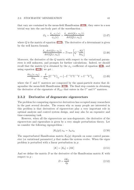
that vary are contained in the mean-field Hamiltonian (1.23), they enter in a non
trivial way into the one-body part of the wavefunction :
O k = δ α k
ψ α (x)
ψ α (x)
= δ α k
det(Q(x, α k )))
det(Q(x, α k ))
(2.47)
where Q is the matrix of equation (2.17). The derivative of a determinant is given
by the well known formula
[ ]
δ αk det(Q(x, α k ))
−1
δQ
= Trace Q (2.48)
det(Q(x, α k ))
δα k
Moreover, the derivative of the Q matrix with respect to the variational parameters
is still unknown, and prompts for further calculations. Indeed, we should
recall that the matrix Q is obtained by the φ ij coefficient of equation (2.8), and
using equation (2.13)) we get :
δφ ij (x, α k )
= δ (
U −1 V ) δα k δα = ( −U −1 U ′ U −1 V + U −1 V ′) (2.49)
ij ij k
where the U and V matrices are composed by the quasi-particle states that diagonalize
the mean-field Hamiltonian (1.23). The final step consists in obtaining
the derivative of the eigenstate of H MF that enters in the U ′ and V ′ matrices.
2.3.2 Derivative of degenerate eigenvectors
The problem for computing eigenvector derivatives has occupied many researchers
in the past several decades. The reason why so many people are interested in
this problem is that derivatives of eigenvectors play a very important role in
optimal analysis and control system design, and may also be an expensive and
time-consuming task.
However, when all the eigenvectors are non-degenerate, the derivative of the
eigenvectors and eigenvalues is given by a very simple perturbation theory. Let
us consider the following eigenproblem :
|K 0 (p)| x 0i = λ 0i x 0i (2.50)
The unperturbated Hamiltonian matrix K 0 (p) depends on some control parameter
(or variational parameter) p that makes the system evolve. When the eigen
problem is perturbed with a linear perturbation in p:
[K] =[K 0 ]+[δK] (2.51)
And we define the matrix D as the derivative of the Hamiltonian matrix K with
respect to p :
D = δK 0
(2.52)
δp