pdf, 9 MiB - Infoscience - EPFL

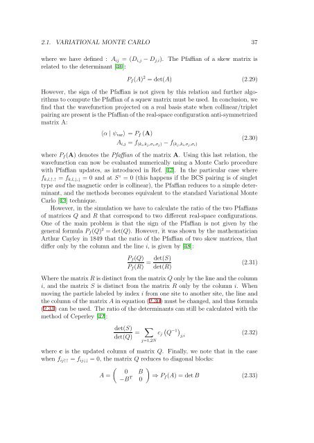
2.1. VARIATIONAL MONTE CARLO 37
wherewehavedefined: A ij =(D i,j − D j,i ). The Pfaffian of a skew matrix is
related to the determinant [46]:
P f (A) 2 =det(A) (2.29)
However, the sign of the Pfaffian is not given by this relation and further algorithms
to compute the Pfaffian of a squew matrix must be used. In conclusion, we
find that the wavefunction projected on a real basis state when collinear/triplet
pairing are present is the Pfaffian of the real-space configuration anti-symmetrized
matrix A:
〈α | ψ var 〉 = P f (A)
A i,j = f (ki ,k j ,σ i ,σ j ) − f (kj ,k i ,σ j ,σ i )
(2.30)
where P f (A) denotes the Pfaffian of the matrix A. Using this last relation, the
wavefunction can now be evaluated numerically using a Monte Carlo procedure
with Pfaffian updates, as introduced in Ref. [47]. In the particular case where
f k,l,↑,↑ = f k,l,↓,↓ =0andatS z = 0 (this happens if the BCS pairing is of singlet
type and the magnetic order is collinear), the Pfaffian reduces to a simple determinant,
and the methods becomes equivalent to the standard Variational Monte
Carlo [42] technique.
However, in the simulation we have to calculate the ratio of the two Pfaffians
of matrices Q and R that correspond to two different real-space configurations.
One of the main problem is that the sign of the Pfaffian is not given by the
general formula P f (Q) 2 =det(Q). However, it was shown by the mathematician
Arthur Cayley in 1849 that the ratio of the Pfaffian of two skew matrices, that
differ only by the column and the line i, is given by [48]:
P f (Q)
P f (R) = det(S)
det(R)
(2.31)
Where the matrix R is distinct from the matrix Q only by the line and the column
i, and the matrix S is distinct from the matrix R only by the column i. When
moving the particle labeled by index i fromonesitetoanothersite,thelineand
the column of the matrix A in equation (2.30) must be changed, and thus formula
(2.31) can be used. The ratio of the determinants can still be calculated with the
method of Ceperley [42]:
det(S)
det(Q) =
∑
j=1,2N
c j
(
Q
−1 ) j,i
(2.32)
where c is the updated column of matrix Q. Finally, we note that in the case
when f ij↑↑ = f ij↓↓ = 0, the matrix Q reduces to diagonal blocks:
( )
0 B
A =
−B T ⇒ P
0
f (A) =detB (2.33)