CASINO manual - Theory of Condensed Matter

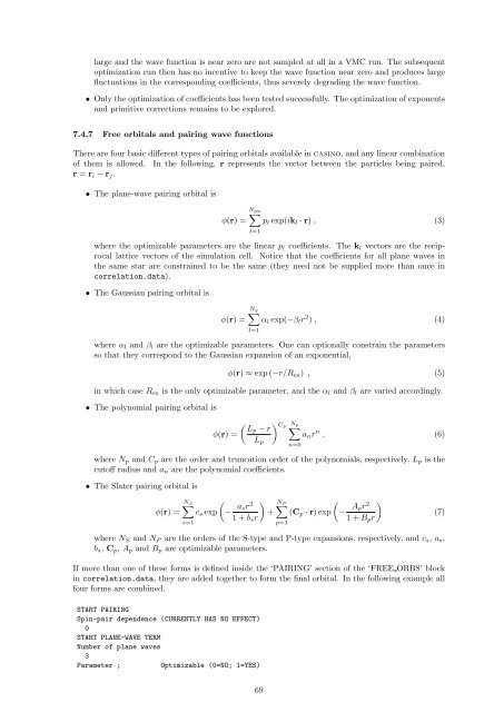
large and the wave function is near zero are not sampled at all in a VMC run. The subsequent
optimization run then has no incentive to keep the wave function near zero and produces large
fluctuations in the corresponding coefficients, thus severely degrading the wave function.
• Only the optimization of coefficients has been tested successfully. The optimization of exponents
and primitive corrections remains to be explored.
7.4.7 Free orbitals and pairing wave functions
There are four basic different types of pairing orbitals available in casino, and any linear combination
of them is allowed. In the following, r represents the vector between the particles being paired,
r = r i − r j .
• The plane-wave pairing orbital is
N pw
∑
φ(r) = p l exp(ik l · r) , (3)
l=1
where the optimizable parameters are the linear p l coefficients. The k l vectors are the reciprocal
lattice vectors of the simulation cell. Notice that the coefficients for all plane waves in
the same star are constrained to be the same (they need not be supplied more than once in
correlation.data).
• The Gaussian pairing orbital is
N g
∑
φ(r) = α l exp(−β l r 2 ) , (4)
l=1
where α l and β l are the optimizable parameters. One can optionally constrain the parameters
so that they correspond to the Gaussian expansion of an exponential,
φ(r) ≈ exp (−r/R ex ) , (5)
in which case R ex is the only optimizable parameter, and the α l and β l are varied accordingly.
• The polynomial pairing orbital is
( ) Cp N
Lp − r ∑ p
φ(r) =
a n r n , (6)
L p
where N p and C p are the order and truncation order of the polynomials, respectively, L p is the
cutoff radius and a n are the polynomial coefficients.
n=0
• The Slater pairing orbital is
∑N S
φ(r) = c s exp
(− a sr 2 )
∑N P
+ (C p · r) exp
(− A pr 2 )
1 + b s r
1 + B p r
s=1
p=1
(7)
where N S and N P are the orders of the S-type and P-type expansions, respectively, and c s , a s ,
b s , C p , A p and B p are optimizable parameters.
If more than one of these forms is defined inside the ‘PAIRING’ section of the ‘FREE ORBS’ block
in correlation.data, they are added together to form the final orbital. In the following example all
four forms are combined.
START PAIRING
Spin-pair dependence (CURRENTLY HAS NO EFFECT)
0
START PLANE-WAVE TERM
Number of plane waves
3
Parameter ;
Optimizable (0=NO; 1=YES)
69