CASINO manual - Theory of Condensed Matter

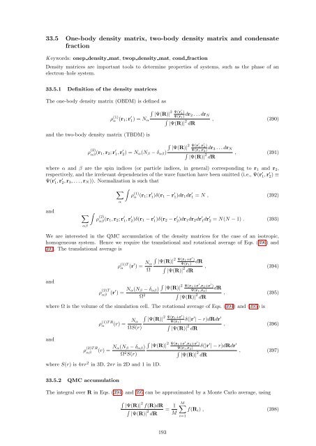
33.5 One-body density matrix, two-body density matrix and condensate
fraction
K eywords: onep density mat, twop density mat, cond fraction
Density matrices are important tools to determine properties of systems, such as the phase of an
electron–hole system.
33.5.1 Definition of the density matrices
The one-body density matrix (OBDM) is defined as
∫
2 Ψ(r |Ψ(R)| ′ 1 )
α (r 1 ; r ′ Ψ(r
1) = N dr 1) 2 . . . dr N
α ∫
|Ψ(R)| 2 dR
ρ (1)
, (390)
and the two-body density matrix (TBDM) is
∫
2 Ψ(r |Ψ(R)| ′ 1 ,r′ 2 )
ρ (2)
αβ (r 1, r 2 ; r ′ 1, r ′ Ψ(r
2) = N α (N β − δ αβ )
dr 1,r 2) 3 . . . dr N
∫
|Ψ(R)| 2 dR
, (391)
where α and β are the spin indices (or particle indices, in general) corresponding to r 1 and r 2 ,
respectively, and the irrelevant dependencies of the wave function have been omitted (i.e., Ψ(r ′ 1, r ′ 2) ≡
Ψ(r ′ 1, r ′ 2, r 3 , . . . , r N )). Normalization is such that
∑
∫
ρ (1)
α (r 1 ; r ′ 1)δ(r 1 − r ′ 1)dr 1 dr ′ 1 = N , (392)
α
and
∑
∫
αβ
ρ (2)
αβ (r 1, r 2 ; r ′ 1, r ′ 2)δ(r 1 − r ′ 1)δ(r 2 − r ′ 2)dr 1 dr 2 dr ′ 1dr ′ 2 = N(N − 1) . (393)
We are interested in the QMC accumulation of the density matrices for the case of an isotropic,
homogeneous system. Hence we require the translational and rotational average of Eqs. (390) and
391. The translational average is
and
ρ (1)T
α (r ′ ) = N α
Ω
∫
2 |Ψ(R)|
Ψ(r 1+r ′ )
Ψ(r 1)
dR
∫
|Ψ(R)| 2 , (394)
dR
∫
ρ (2)T
αβ (r′ ) = N 2
α(N β − δ αβ ) |Ψ(R)|
Ψ(r 1+r ′ ,r 2+r ′ )
Ψ(r 1,r 2)
dR
Ω 2 ∫
|Ψ(R)| 2 , (395)
dR
where Ω is the volume of the simulation cell. The rotational average of Eqs. (394) and (395) is
ρ (1)T R
α (r) = N α
ΩS(r)
∫
2 |Ψ(R)|
Ψ(r 1+r ′ )
Ψ(r 1)
δ(|r ′ | − r)dRdr ′
∫
|Ψ(R)| 2 , (396)
dR
and
∫
ρ (2)T R
αβ
(r) = N 2
α(N β − δ αβ ) |Ψ(R)|
Ψ(r 1+r ′ ,r 2+r ′ )
Ψ(r 1,r 2)
δ(|r ′ | − r)dRdr ′
Ω 2 ∫
S(r)
|Ψ(R)| 2 , (397)
dR
where S(r) is 4πr 2 in 3D, 2πr in 2D and 1 in 1D.
33.5.2 QMC accumulation
The integral over R in Eqs. (394) and 395 can be approximated by a Monte Carlo average, using
∫
|Ψ(R)| 2 f(R)dR
∫
|Ψ(R)| 2 dR
= 1 M
M∑
f(R i ) , (398)
i=1
193