CASINO manual - Theory of Condensed Matter

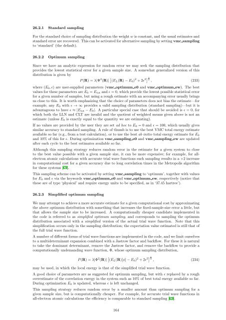
26.2.1 Standard sampling
For the standard choice of sampling distribution the weight w is constant, and the usual estimates and
standard error are recovered. This can be activated for alternative sampling by setting vmc sampling
to ‘standard’ (the default).
26.2.2 Optimum sampling
Since we have an analytic expression for random error we may seek the sampling distribution that
provides the lowest statistical error for a given sample size. A somewhat generalized version of this
distribution is given by
P (R) = λ|Ψ 2 (R)| [ (E L (R) − E 0 ) 2 + 2ɛ 2] 1 2
, (233)
where (E 0 , ɛ) are user-supplied parameters (vmc optimum e0 and vmc optimum ew). The best
values for these parameters are E 0 = E tot and ɛ = 0, which provide the lowest possible statistical error
for a given number of samples, but using a rough estimate with an accompanying error usually brings
us close to this. It is worth emphasizing that the choice of parameters does not bias the estimate—for
example, any E 0 with ɛ → ∞ provides a valid sampling distribution (standard sampling)—but it is
advantageous to have ɛ ≈ |E tot − E 0 |. A particular special case that should be avoided is ɛ = 0, for
which both the LLN and CLT are invalid and the quotient of weighted means given above is not an
estimate (unless E 0 is exactly equal to the quantity we are estimating).
If no values are provided by the user they are set ad hoc to E 0 = 0 and ɛ = 100, which usually gives
similar accuracy to standard sampling. A rule of thumb is to use the best VMC total energy estimate
available so far (e.g., from a test calculation), or to use the best ab initio total energy estimate for E 0
and 10% of this for ɛ. During optimization vmc sampling e0 and vmc sampling ew are updated
after each cycle to the best estimates available so far.
Although this sampling strategy reduces random error in the estimate for a given system to close
to the best value possible with a given sample size, it can be more expensive; for example, for allelectron
atomic calculations with accurate trial wave functions such sampling results in a ×2 increase
in computational cost for a given accuracy due to long correlation times in the Metropolis algorithm
for these systems [69].
This sampling scheme can be activated by setting vmc sampling to ‘optimum’, together with values
for E 0 and ɛ via the keywords vmc optimum e0 and vmc optimum ew, respectively (notice that
these are of type ‘physical’ and require energy units to be specified, as in ‘37.45 hartree’).
26.2.3 Simplified optimum sampling
We may attempt to achieve a more accurate estimate for a given computational cost by approximating
the above optimum distribution with something that increases the fixed-sample-size error a little, but
that allows the sample size to be increased. A computationally cheaper candidate implemented in
the code is referred to as simplified optimum sampling, and corresponds to sampling the optimum
distribution associated with a simplified version of the actual trial wave function. Note that this
simplification occurs only in the sampling distribution; the expectation value estimated is still that of
the full trial wave function.
A number of different forms of trial wave functions are implemented in the code, and we limit ourselves
to a multideterminant expansion combined with a Jastrow factor and backflow. For these it is natural
to take the dominant determinant, remove the Jastrow factor, and remove the backflow to provide a
computationally undemanding wave function, Φ, whose optimum sampling distribution,
P (R) = λ|Φ 2 (R)| [ (E L (R)[φ] − E 0 ) 2 + 2ɛ 2] 1 2
, (234)
may be used, in which the local energy is that of the simplified trial wave function.
A good choice of parameters are as suggested for optimum sampling, but with ɛ replaced by a rough
overestimate of the correlation energy in the system such as 10% of best total energy available so far.
During optimization E 0 is updated, whereas ɛ is left unchanged.
This sampling strategy reduces random error by a smaller amount than optimum sampling for a
given sample size, but is computationally cheaper. For example, for accurate trial wave functions in
all-electron atomic calculations the efficiency is comparable to standard sampling [69].
164